From human mobility to renewable energies

Abstract

We address and discuss recent trends in the analysis of big data sets, with the emphasis on studying multiscale phenomena. Applications of big data analysis in different scientific fields are described and two particular examples of multiscale phenomena are explored in more detail. The first one deals with wind power production at the scale of single wind turbines, the scale of entire wind farms and also at the scale of a whole country. Using open source data we show that the wind power production has an intermittent character at all those three scales, with implications for defining adequate strategies for stable energy production. The second example concerns the dynamics underlying human mobility, which presents different features at different scales. For that end, we analyze $12$-month data of the Eduroam database within Portuguese universities, and find that, at the smallest scales, typically within a set of a few adjacent buildings, the characteristic exponents of average displacements are different from the ones found at the scale of one country or one continent.

1 Big data: the emergence of a new paradigm

In some sense, the notion of Information Age is slowly fading from the perception of our society. For decades, national and international research has been creating impressive amounts of data, and often from various unrelated measurement sourcesCERN . Computational methods have been serving the needs of the scientific community and the need for higher computational power has driven the invention of more efficient computational codes and triggered the development of new hardware. Simultaneously, the internet has been instrumental in fostering international research collaborations and divulging scientific knowledge.

Today, obtaining data is no longer a problem. Information is there, available for everyone at any time. Given the computational power of today’s computers and clusters, even single research groups can create and store large data volumes. The challenge in today’s research is more often what to do with the data we have. How to manage all the information we have in such large data sources? Which phenomena can we now study? The recent technological progress together with the new challenges naturally lead to a new paradigm in computational sciences, which is partially described by the term big data.

In this paper we discuss the utility of big data for approaching the empirical study of phenomena up to now unreachable. We discuss the usage of big data in the study of two specific phenomena, that up to now were unreachable, namely wind energy production and human mobility. These phenomena cover several spatial scales coupled with each other, ranging from a few meters up to several hundreds of kilometers. Such phenomena are usually called multiscale phenomena.

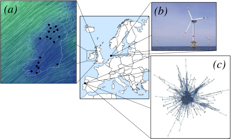
Figure 1: (Color online) Big data sets and their application to multiscale phenomena: wind energy production at the scale of (a) one wind farm or an entire country and of (b) single wind turbines. In (c) human mobility, where one shows a subset of the Eduroam network comprehending the data from University of Minho (January-December 2011), with its workers and students spreaded throughout other Eduroam networks in Portugal.

Big data is generally understood as notion of massive amounts of data, often of social and economical origin and/or relevance, whose storage, loading into memory, or computational processing by far exceeds the computational power of a single PC, and therefore requires the use of parallel file systems and processors and the development of the corresponding parallelized software, not only for algorithmic computation, but also for storing and accessing the data, see bigdata about the concept and nelson2008 about how it existed even before computers. The new big data paradigm is therefore rooted in four technological and societal developments.

First, rapid and low-cost electronics for sensoring and data acquisition allow us to obtain the so-called rise of electronics: modern and low-cost electronic data acquisition and sensoring devices give the technological possibility to acquire in real time large-scale experimental, simulational or social data. Important examples are, of course, satellites, cellular phones, D/A converters, and the internet, which itself is a considerable source of social data.

Second, we now achieve data completeness on scales. Among many others one may refer to the example of travel and cell phone data, as well as health data, data from electronic payment systems or high-frequency trading data. In geophysics, meteorological data cover geographically scales as small as a few kilometers up to the entire global scale. When referring to social data the complete demographic databases may be available. In physical phenomena, all relevant scales of physical multiscale problems such as turbulence, multiscale material problems or complex fluids can nowadays possible to be empirically assessed.

Third, it is also necessary to assure data availability as well as computational power for developing data mining procedures. This means that we have on the one hand the technological, organizational, economical and efficient means to centrally store, share and transfer the data. On the other hand, the practical usefullness of the stored data is strongly influenced by the technological means to efficiently and rapidly find patterns in these data.

Finally, one should have a storage and mining system that enables the combination of sources. Today’s technology enables the combination of the aforementioned sources, e.g. location and social interaction from cell phone location and connection data, travel and spending patterns or the combination of meteorological data, wind power generation and electrical network activity.

These mainly tehnological developments have had a strong impact in physics, which has witnessed the establishment of computational method as a third pillar in empirical sciences, next to theory and experimentationhistoryofscience . However, big data is not defined by the magnitude of the data alone, but rather by the statistical complexity of the problem that is being addressed. Of particular interest are multiscale phenomena, since they require typically large amounts of data from different sources.

We start in Sec. 2 by describing in some detail applications of big data for various multiscale phenomena. In Sec. 3 we treat the specific case of big data analysis in wind energy research, comparing the power increments found in the full wind power production data in Ireland with those from a large park in Australia and a single turbine in an off-shore wind farm in Germany’s North Sea (Fig. 1b). In Sec. 4 we approach the problem of the patterns describing human mobility, describing recent results at large scales and showing how they differ from human motion at the smallest scales. Section 5 concludes the paper.

2 Big Data for World-wide and Multiscale Problems

One important aspect in big data is that it enabled physicists to finally treat physical and statistical problems not only in a crude approximation, on a single relevant scale, on a coarse grid, or for a small sample of data, but on a full set of different scales, either in time, in space or in their organizational nature. In this section we discuss briefly some examples of world-wide multiscale data.

One phenomena that can now be approached refers to the entire global data sets for human travel patterns, or social data sets representing entire populations. It is knowngonzaleznature ; brockmannnature that human mobility follows non-Brownian laws when observed at large scales, such as that of an entire country. However, as we show below, for the smallest scales, comprehending streets and few buildings, we find human motion to be almost Brownianadriano .

The international financial marketseconophysics are another example of an extremely interlinked system, with information flow on various time scales, an effect that is ever increasing due to globalization and high speed tradingKenett2013 . It is now well accepted that a realistic description of financial markets can be achieved through agent models, which try to recreate financial interdependencies among a large number of individuals which differ by behavior and available assetslevy_agents . These models allow notably for the description of failure avalanchescruz_financial . An interesting example of the information exchange between different world-wide multiscale systems is the predictive character of human internet searches on stock market tradesPreis2013 . Even when considering only small samples of data sets representing connected agents, analyzing the correlations between them quickly leads to complex problemsLaloux1999 ; plerou_cor . Further examples range from uncovering the correct statistical description of financial time seriesCamargo2013 , as far as they exist in a non-stationary systemmccauley2004 , to devising trading strategies which could mitigate sudden crashesBiondo2013 , to finding regulatory measures which can stabilize the marketscruz_financial .

Nevertheless, an important note is in order here: financial markets are not physical systems. Rather, the principal driving force of markets is profit, where profit is to be gained by – at least partially irrational – individuals competing for advantages in information, and influencing each others’ opinionsKinzel2003 ; sornette2009 . This reaction to new information leads to “reclective” feedback loopssornette2012 and is in strong contrast to the notion of invariant natural laws found in the sciences. As Feynman said fittingly “Imagine how much harder physics would be if electrons had feelings!”, cited in Lo2010 .

Another important field where processes in scale are abundant is geophysics. Here, energy flows across structures spanning several orders of magnitude. Earthquakes, which are essentially a fracturing phenomenon, show a flow of energy release events from the micro- to the macroscale. Present-day state of the art is the microscopic simulation of fracture on the molecular scaleAbraham2003 , real-time observation at the nanoscaleprades2005 , the stochastic or continuum description at the mesoscalekun2006 ; kun2014 , and the statistical description of earthquakes on the fault system or global scalesornette2008 ; Holliday2008 .

Recent advantages in the modeling of fracture of heterogeneous materials could give an answer about the nature of the fracture phase transitionShekhawat2013 . At present, it remains an unresolved problem to correctly understand the details of damage propagation in models of earthquakes and experimental data, e.g. the statistics of intershock sequencesBottiglieri2010 ; Touati2009 , and the recurrence of events and record breakingsDavidsen2008 . The possibility of predicting individual earthquakes remains, however, a subject with an unclear outlookpradhan2005 ; Lippiello2012 ; Main1999 ; Main2012 .

Even on the geological time- and length scales, models exist to describe the formation and phenomenology of geomorphological features, such as river deltasSeybold2007 , coastal dunesduran2013 , watershedsFehr2011 , or coastlinesmorais2011 . The latter two models are based on scaling processes related to percolation and represent long-scale correlations in the formation process.

Similar considerations lead to models of porous rock formationsBiswal2007 , which often carry fossil resources, leading to the question of how these reservoirs can be exploited most efficientlySchrenk2012 . Here simulations of the complex fluid-fluid and fluid-rock interfaces are also needed to gain further insightSucci2001a ; narvaez2010 ; narvaez2013 .

To end this overview of research topics, there is also the problem of wind energy production and its fluctuations in time. Wind energy production is essentially determined by large-scale turbulent atmospheric dynamics and extreme event statistics, two topics that still require a multidisciplinary comprehensive approach, from both the earth sciences Lovejoy2009 ; Donner2009a and physicsFriedrich2011a .

Recently, new insight has been found into how intermittency in wind energy production is preserved when going from the scale of single wind turbines to the scale of entire wind farms and even to the scale of countries having several wind farmsrezassub ; pats ; oli . This has raised new questions on how to stabilize energy production on the scale of large economies. Furthermore, the role of long-range correlations in wind velocities due to meteorological systems on the synoptic scale remains an open questionvitor_wr .

As one can see, we find world-wide multiscale processes spanning from social systems, through biology, and geological processes. In the following, we will take a closer look at two of these phenomena. The first one, world-wide wind-power generation, not only is affected by large-scale meteorological processes, but then it also links the produced power to continental electric grids. The second phenomenon is human mobility, and its importance is intrinsically linked to multiscale multiscale technological applications, e.g. flight management and cell phone networks, as well as to biology, when addressing the world-wide spreading of diseases.

3 Big data in geophysics: the example of wind energy

Wind energy is one of the best candidates to answer the world-wide energetic problemjohnsonWindBook , and simultaneously it is a “clean” source of energy. However it has a drawback: it reflects the turbulent nature of the wind itself. As it is knownwindenergyhandbook , since wind speed presents non-Gaussian fluctuations in time, the power output of one turbine also shows this intermittent behaviorpatrickprl making predictions of energy production rather difficult. Moreover, power grids fed only from wind energy alone would be unstable, with periods of large production alternated with periods of very low production. These facts raise challenges to the wind power producers who need to trade on these variations in the electricity marketsteresaspaper . Large fluctuations in the energy produced can impede the matching to the committed energy.

These large fluctuations are a function of the time scale of the observation and disappear for large enough time increments. Indeed, similar to what happens in the stock marketnaturepeinke , while the increments of power production evidence significant deviations from the Gaussian regime with heavy tails, for large time increments these tails disappear. Figure 2a shows the increment statistics of the power output defined as

$$\Delta P_{\tau}(t)=P(t+\tau)-P(t),$$ (1)

where $P(t)$ is the power output measured at time-step $t$ and $\tau$ is a fixed time-gap between two measures. As we see in Fig. 2a the heavy-tails disappear as the time-gap increases from one second up to more than one hour.

However, expected returns in power production must sometimes be taken within a time period shorter than one hour, increasing the risk associated with the expected values. Recently, some variants of the standard risk-return approach have been proposedteresaspaper for solving this shortcoming.

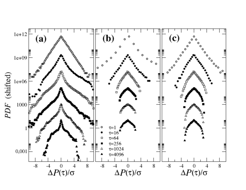
Figure 2: Big data sets and its application to multiscale phenomena: wind energy production at the scale of (a) single wind turbines (in units of seconds), of (b) a large wind farm in Australia (in units of $5$ minutes) and of (c) an entire country, Ireland, for which a detrending procedure was applied as described in oli (in units of $15$ minutes). In all plots PDFs are shifted vertically for better visualization.

The single turbine data was provided by Senviondata and comprehends the full month of January 2013, measured at one wind turbine of the Alpha Ventus wind farm in Germany, located approximately at $54.3^{o}$N-$6.5^{o}$W.

Another way to “smoothen out” the impact of these short-term fluctuations could be to add more turbines to a given network. If a single turbine would show Gaussian statistics in its power output, even if they were not completely uncorrelated, then, according to the central limit theorem, the heavy-tails of the distribution should disappear as one considers the joint power output of more and more turbines.

However what we find in the case of wind energy production is an intermittent behavior at all three scales. Figure 2b and 2c show the distribution of power increments, aggregating data of an entire wind farm in Australia and of all wind farms in Ireland, respectively. As one sees in Fig. 2 the large fluctuations of energy production at the level of one single turbine are also observed on the power production of an entire wind farm or on the sum of all wind farms within one country. Similar results were observed in previous workspats ; oli .

One possible cause for the emergence of heavy tails at several spatial scales is the existence of uncorrelated, stable-Lévy distributed sources. Another cause is the existence of correlations between the wind conditions at all these scales. In the case of Ireland, the wind flux streams drawn in Fig. 1a clearly sweep the entire country in a similar way. In other words, Ireland lies typically in the same weather system and therefore the wind shows the same features whether it is observed at one single turbine, in an entire wind farm or as a pattern in a full country.

By taking adjacent countries comprising an area larger than the entire weather system, wind turbines and wind farms in that larger area will be differently affected by the weather system and therefore will eventually lead to uncorrelated wind conditions. Consequently, having “uncorrelated” wind turbines and wind farms opens the possibility for more stable power grids and a better matching between produced and committed energy. Moreover, recently, it has been shown that combining different renewable energy sources, such as wind and solar sources, would allow to obtain a more constant combined power production raterezassub .

4 Big data in society: the example of human mobility

Understanding human motion from small scales, such as buildings and streets up to larger ones comprising cities, countries and continents, is fundamental for a variety of topics such as spreading of diseases, optimization of telecommunication networks, urban planning, and tourism management. Several groups have been modeling human motiongonzaleznature ; brockmannnature ; ahas2006 ; ahas2007 , showing that human traveling distances within the USA decay as a power-lawbrockmannnature , and that there is one single probability distribution for time returns to previous locationsgonzaleznature .

In Ref. brockmannnature the authors use data obtained from an online tracker system where registered users reported the observation of marked US dollars bills, while in Ref. gonzaleznature one data set is used, containing positioning records of around $10^{5}$ users of a cellular network. While these data sets were important to uncover mobility patterns at the level of the USA, two drawbacks of the data sets used so far should be stressed. First, in both cases the data records correspond to positions collected at sparse time steps and no continuous tracking is possible. Second, the accuracy of position measurement were constrained to e.g. the cell ID with a coverage area over several square kilometers. Therefore, human mobility at smaller scales still lacks to be addressed, mostly because of the nature of available data.

In this section we analyze a large data set of individual locations in a continuous time tracking system at scales as small as buildings and city streets. The data set we analyze is extracted from the Eduroam networks at Portuguese Universities (see Fig. 1c), a part of a large data set comprising entire Europe. By analyzing the Eduroam net at the level of one single university we achieve the smallest scale at which human motion takes place, as addressed in Refs. adriano ; adriano1 ; adriano2 ; adriano3 .

The Eduroam data set comprises one year of collected information with a sample frequency of one second, a time step that enables to assume the data as continuous monitoring of human motion. The spatial resolution is of the order of a few meters, the typical distance between adjacent access points (APs). At these small scales one expects that human trajectories are closer to the Brownian regime than what is observed at the larger spatial scales reported in Refs. gonzaleznature ; brockmannnature . We will show that indeed this is the case.

The data set comprehends an Eduroam RADIUS log file from the University of Minho (Portugal) infrastructure, including the full year of 2011. The file contains a total of $15,892,009$ data records $7,937,245$ of them refer to “start-events” and $7,954,764$ refer to “stop-events”. A few of these records ($0.65\%$) have been filtered, since they are incomplete or do not represent unique Access Points or unique Stations. After filtering, we obtain $7,902,828$ records for processing and analysis.

First, we extract the topological structure of the network of APs. More than the spatial distances between APs joined by paths such as stairs, corridors or open spaces, we deal with a topological distance between APs that reflects how often people tend to move between each pair of APs. Such an approach in constructing a complex network has been applied frequently to address social and environmental problemslind05 ; gonzalez06 ; gonzalez06b ; lind07 ; lind07b . Still, we introduce here a novel procedure for extracting the network on which persons move directly from empirical data. Our approach can be easily extended to the full European Eduroam data set.

Using all the records at University of Minho we construct a weighted AP network considering all $723$ APs detected during each full month of 2011.

For extracting the AP network, we consider the Eduroam database as an output file with three single fields for each register, namely the user $i$ (or alternatively the device one user is using when connected to the net), the AP $I$, where the user is connected to and the time $t$ in units of the time step $\Delta t=1$ second, which is typically the size of the smallest time lag between successive registers. Henceforth, small letters indicate properties of the users, while capital letters indicate properties of the APs.

We start by counting the total number of connected users to one particular AP $I$ at time step $t$, yielding the AP fitness $G_{I}(t)$. At each time-step $t$, $G_{I}(t)$ at AP $I$ equals the total number of associations occurred at $I$ minus the total number of disassociations, occurred within the full time span from the beginning of the observation period up to time $t$. The full time span considered is of $24$ hours, beyond which we assume that each user cannot be further connected. Our results have shown that neglecting sessions longer than 24 hours has no significant impact in the following analysisadriano .

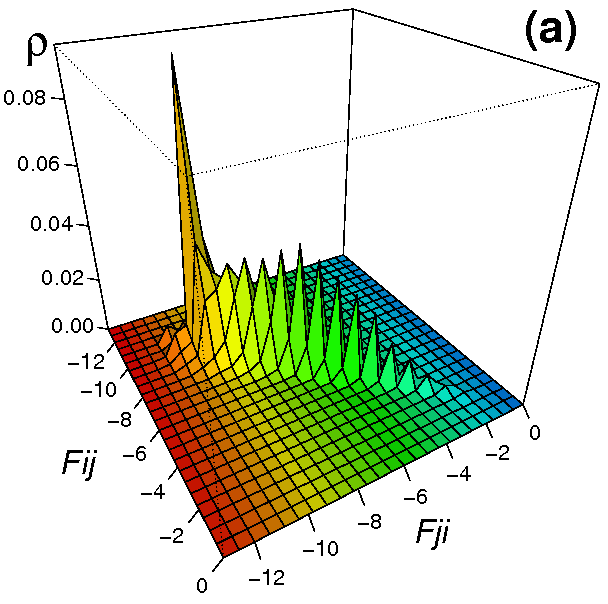
Figure 3: (a) Histogram of the average flux between each pair of APs in both directions, showing a symmetry relation $\langle F_{IJ}\rangle\simeq\langle F_{JI}\rangle$ which supports the definition for the (symmetric) weights $W_{IJ}$ in the AP network (see text). (b) Number $M$ of AP switches as a function of the time window $\Delta T$, defining the flux $F_{IJ}=dM/d(\Delta T)\sim M/\Delta T$ (see Eq. (2)) which is approximately constant for $\Delta T$. Shown is the slope for four different pairs $IJ$ of APs taken at the first day of 2011. (c) Weight average $\langle W\rangle$ and standard deviation $\sigma_{W}$ as a function of month, using January as the reference month.

The network of APs has a weight matrix defined by the weights $W_{IJ}=1/D_{IJ}$, where $D_{IJ}=D_{JI}$ is a proper topological distance between APs $I$ and $J$. Since we do not have the location of the APs and we do not know exactly the full number of constraints that condition the displacement from one AP to the next one, we introduce a topological distance as follows.

First, we compare the average fitness $\langle G_{I}(t)\rangle$ at each AP $I$ and the instantaneous flux $F_{IJ}$ between $I$ and $J$ defined as

$$F_{IJ}(t)=\frac{dM_{IJ}(t,\Delta T)}{d(\Delta T)},$$ (2)

where $M_{IJ}(t,\Delta T)$ is the number of users that associate to AP $J$ after disassociating from AP $I$, within a time window $\Delta T\lesssim 1$ day start at time $t$. Figure 3a shows the frequency of each flux strength $F_{IJ}$, in one direction, and the flux $F_{JI}$, in the opposite direction, showing a symmetry, $F_{IJ}\sim F_{JI}$. As shown in Fig. 3b, for four different pairs $IJ$ of APs, the average flux is approximately constant within time windows up to one day. Therefore, to reduce the computation time, we consider henceforth the average flux within $\Delta T=4$ hours as an estimate of the flux between each pair of APs to reduce the computation time.

From these quantities, $\langle F_{IJ}\rangle$ and $\langle G_{I}(t)\rangle$ one finally defines the weight of each connection as

$$W_{IJ}\equiv\frac{1}{D_{IJ}}=\tfrac{1}{2}\left(\frac{\langle F_{IJ}(t)\rangle}{\langle G_{I}(t)\rangle}+\frac{\langle F_{JI}(t)\rangle}{\langle G_{J}(t)\rangle}\right).$$ (3)

From such a definition the weights are properly averaged over their fitness and simultaneously contain the same symmetry as the fluxes, $W_{IJ}=W_{JI}$ (see Fig. 3a).

Since there are seasonal fluctuations from month to month, as shown in Fig. 3c, the average fitness at each AP is considered for a time window of one month and repeated for every month during the entire year. A similar approach has been used for the calculation of the average flux, which yields one AP network for each month. The weight average $\langle W\rangle$ – over all AP connections $IJ$ – varies from month to month as well as the corresponding deviations

$$\sigma_{W}(t)=\left(\frac{1}{N-1}\sum_{connections}\left(W_{IJ}(t)-\langle W\rangle(0)\right)^{2}\right)^{1/2}$$ (4)

from a reference month average, chosen to be January. While some significant variations are observed during the summer vacations, the normalized deviations $\sigma_{W}/\langle W\rangle$ are approximately constant. This result also highlights the temporal evolution on the usage of the network, with more and more users accessing the network and also more APs being deployed to improve the network capacity.

Figure 4: Average shortest distance $r(t)$ of human trajectories within Portuguese Universities as a function of time (in seconds). While for short times people tend to remain at the same place (connected to the same AP), with $r_{min}$, beyond around $20$ minutes there is a marked scaling of the displacement with time, $r\sim t^{\delta}$ with $\delta\sim 0.5$, describing the normal Brownian diffusion regime.

Having defined the weight, one can immediately obtain the matrix of topological distances $D_{IJ}=1/W_{IJ}$ between APs. We symbolize the position of one individual $i$ at time $t$ through its trajectory as $r_{i}(t)$ with reference to an initial position, labeled AP $I_{0}$. In other words, if person $i$ at time $t$ is connected to AP $I$, its position is $D_{I_{0}I}$ (see Eq. (3) and Eq. (5) below). For practical purposes we assume that one person corresponds to one single trajectory, and thus label both trajectories and individuals with the same label $i$. Each trajectory followed by one person is defined by the succession of APs and by the corresponding shortest distances $D_{I_{0}I}$ to the initial AP $I_{0}$.

Keeping track of the distance from the initial position, and averaging over all trajectories in the data sets yields the average shortest distance from the initial position computed as

$$r(t)=\langle r_{i}(t)\rangle_{traj}=\langle D_{I_{0}I}\rangle_{traj}=\frac{1}{N_{traj}(t)}\sum_{i=1}^{N_{traj}(t)}r_{i}(t),$$ (5)

with $i$ labeling one of the $N_{traj}(t)$ individual trajectories observed at each time $t$ starting at $t_{0}$, with steps of $\Delta t=1$ second.

As shown in Fig. 4, while for short and long times the displacement tends to remain approximately constant, for middle times $r(t)$ increases with time $t$ as a power law $r\sim t^{\delta}$ with $\delta\simeq 0.48\pm 0.03$. This exponent is equal, within numerical error, to the one known to characterize Brownian diffusion, contrary to what is observed for large scale mobility, as reported in Refs. gonzaleznature ; brockmannnature . Seemingly, people move according to large jumps within large time-spans and over large spatial scales, but they tend to diffuse randomly with small jumps when trajectories are tracked in shorter times and over the smallest spatial scales.

5 Discussion and conclusions

In this paper we focus on possible applications of big data set analysis to empirically approach multiscale phenomena. Providing a brief discussion in the fields of sociology, finance, economics, physics and geophysics, we discuss in detail two particular phenomena, namely fluctuations in wind energy production and human mobility.

When assessing data of wind energy production we observed a large intermittency in the increments of wind power at scales up to the country level. This intermittent power production raises difficulties in the energy market for determining the optimal committed power outputs. Two ways to overcome this problem could be proposed.

One possibility is to construct power grids based in wind farms typically distributed over more than one country, in order to sum less correlated power outputs. Such possibility has two inconveniences. First, countries within Europe should agree on long-term energy policies and commit to the corresponding investments. Second, even if such an agreement is met for merging into a European joint stable power grid, several problems related to storage and distribution in large power grid are still to be solvedandre2013 .

Another possibility would be to join different sources of renewable energy, for example solar and wind energy within one country. This possibility was recently proposedrezassub although analysis of data at larger scales might provide insight on how reliable these pioneering studies are.

For human mobility we considered the Eduroam data set at the smallest scales where individuals move along streets and between buildings, in this case, within the University of Minho (Portugal). While it is known that a power-law distribution is found for the distance from starting position when one keeps track of individual trajectories at large scales, at small scales we found that human mobility closely follows Brownian motion. The mobility network was extracted from the empirical data directly by measuring average fluxes of people between adjacent access points inside the university.

Since the Eduroam data base covers the whole of Europe, a possible next step would be to consider the joint data base of several European universities. By properly matching the mask IDs and similar quantities at different universities, one would be able to keep track of individuals throughout Europe and apply the framework described above to data sets comprising larger and larger areas. Since the mobility of faculty, researchers and students is becoming higher due to European programs such as Erasmus, one should expect sufficient statistics in the Eduroam databases at several spatial scales. Consequently, one should be able to observe the transition from Brownian to non-Brownian motion, postulated in this paper.

References

- (1) G. Brumfiel, Nature 282, 8 (2011).
- (2) K.N. Cukier, V. Mayer-Schoenberger, The Rise of Big Data (Foreign Affairs, May/June 2013).
- (3) S. Nelson, Nature 455, 36 (2008).
- (4) A. Barberousse, S. Franceschelli and C. Imbert, Synthese 169, 557 (2009).
- (5) M.C. González, C.A. Hidalgo and A.-L. Barabási, Nature 453, 779 (2008).
- (6) D. Brockmann, L. Hufnagel and T. Geisel, Nature 439, 462 (2006).
- (7) A. Moreira and P.G. Lind, “Human mobility patterns at the smallest scales”, submitted (2014).
- (8) R.N. Mantegna and H.E. Stanley, Introduction to econophysics: correlations and complexity in finance (Cambridge Univ. Press, 2000).
- (9) D.Y. Kenett, E. Ben-Jacob, H.E. Stanley, and G. Gur-Gershgoren, Sci. Rep. 3, 2110 (2013).
- (10) D. Sornette, Why stock markets crash: critical events in complex financial systems (Princeton University Press, 2009).
- (11) V. Filimonov and D. Sornette, Phys. Rev. E 85 056108 (2012).
- (12) H. Levy, M. Levy, and S. Solomon, Microscopic simulation of financial markets: from investor behavior to market phenomena (Academic Press, 2000).
- (13) J.P. Da Cruz and P.G. Lind, The European Physical Journal B 85, 1 (2012).
- (14) T. Preis, H.S. Moat and H.E. Stanley, Sci. Rep. 3, 1684 (2013).
- (15) L. Laloux, P. Cizeau, J.P. Bouchaud, and M. Potters, Phys. Rev. Lett. 83 1467 (1999).
- (16) V. Plerou, P. Gopikrishnan, B. Rosenow, A.N. Amaral, and H.E. Stanley, Phys. Rev. Lett. 83, 1471 (1999).
- (17) S. Camargo, S.M.D. Queirós, and C. Anteneodo, Eur. Phys. J. B 86, 159 (2013).
- (18) J.L. McCauley, Dynamics of markets: econophysics and finance (Cambridge University Press, 2004).
- (19) A. Emanuele, A. Pluchino, A. Rapisarda, and D. Helbing “Stopping Financial Avalanches By Random Trading”, available at http://arxiv.org/abs/1309.3639 (2013).
- (20) W. Kinzel, I. Kanter, “Disorder Generated by Interacting Neural Networks: Application to Econophysics and Cryptography”, J. Phys. A 36, 11173 (2003).
- (21) A.W. Lo, “Warning: Physics Envy May Be Hazardous to Your Wealth!”, Journal of Investment Management (JOIM), Second Quarter (2010).
- (22) F. Abraham, Advances in Physics 52, 727 (2003).
- (23) F. Kun, R.C. Hidalgo, F. Raischel, H.J. Herrmann, Int. J. Frac. 140 255 (2006).
- (24) F. Kun, I. Varga, S. Lennartz-Sassinek, and I.G. Main, Phys. Rev. Lett. 112, 065501 (2014).
- (25) D. Sornette, M.J. Werner, “Statistical Physics Approaches to Seismicity”, In Extreme Environmental Events, pp 825-843 (Springer New York, 2011).
- (26) J.R. Holliday, D.L. Turcotte, and J.B. Rundle, Pure and Applied Geophysics 165, 1003 (2008).
- (27) A. Shekhawat, S. Zapperi, and J.P. Sethna, Phys. Rev. Lett. 110, 185505 (2003).
- (28) M. Bottiglieri, L. de Arcangelis, C. Godano, and E. Lippiello, Phys. Rev. Lett. 104, 158501 (2010).
- (29) S. Touati, M. Naylor, and I.G. Main, Phys. Rev. Lett. 102, 168501 (2009).
- (30) J. Davidsen, P. Grassberger, and M. Paczuski, Phys. Rev. E 77, 066104 (2008).
- (31) S. Pradhan, A. Hansen, and P.C. Hemmer, Phys. Rev. Lett. 95, 125501 (2005).
- (32) E. Lippiello, W. Marzocchi, L. de Arcangelis, and C. Godano, Sci. Rep. 2, 846 (2012).
- (33) I. Main, “Is the Reliable Prediction of Individual Earthquakes a Realistic Scientific Goal”, in Nature Debates (1999); available at www.nature.com/nature/debates/earthquake/equake_frameset.html.
- (34) I.G. Main, M. Naylor, Eur. Phys. J. Spec. Top. 205, 183 (2012).
- (35) E. Fehr, D. Kadau, J.S. Andrade Jr, and H.J. Herrmann, Phys. Rev. Lett. 106, 048501 (2011).
- (36) P.A. Morais, E.A. Oliveira, N.A.M. Araújo, H.J. Herrmann, and J.S. Andrade Jr., Phys. Rev. E 84, 016102 (2011).
- (37) H. Seybold, J.S. Andrade, and H.J. Herrmann, PNAS 104, 16804 (2007).
- (38) B. Biswal, P.-E. Øren, R. Held, S. Bakke, and R. Hilfer, Phys. Rev. E 75 1 (2007).
- (39) K.J. Schrenk, N.A.M. Araújo, and H.J. Herrmann, Sci. Rep. 2, 751 (2012).
- (40) S. Succi, O. Filippova, Comp. Sci. & Engin. 3, 26 (2001).
- (41) A. Narváez, T. Zauner, F. Raischel, R. Hilfer, J. Harting, J. Stat. Mech. 11, P11026 (2010).
- (42) A. Narváez, K. Yazdchi, S. Luding, J. Harting, J. Stat. Mech. 2, P02038 (2013).
- (43) S. Lovejoy, D. Schertzer, V. Allaire, T. Bourgeois, S. King, J. Pinel, and J. Stolle, Geophys. Res. Lett. 36, L01801 (2009).
- (44) R. Donner, S. Barbosa, J. Kurths, and N. Marwan, Eur. Phys. J. Sp. Top. 174 1 (2009).
- (45) R. Friedrich, J. Peinke, M. Sahimi, and M.R.R. Tabar, Phys. Rep. 506 87 (2011).
- (46) M.R.R. Tabar, M. Anvari, P. Milan, G. Lohmann, E. Lorenz, and J. Peinke, “Renewable Power from Wind and Solar: Their Resilience and Extreme Events”, submitted (2013).
- (47) P. Milan, A. Morales, M. Wächter, and J. Peinke, “Wind Energy: A Turbulent, Intermittent Resource”, In Wind Energy-Impact of Turbulence, pp 73-78 (Springer, Berlin Heidelberg, 2014).
- (48) O. Kamps, “Characterizing the Fluctuations of Wind Power Production by Multi-time Statistics”, In Wind Energy-Impact of Turbulence, pp 67-72 (Springer, Berlin Heidelberg, 2014).
- (49) P. Costa, V.V. Lopes, and A. Estanqueiro, “Impact of Weather Regimes on the Wind Power Ramp Forecast”, 12th International Workshop on Large-Scale Integration of Wind Power into Power Systems as well as on Transmission Networks for Offshore Wind Power Plants, London October 22-24 (London, UK, 2013).
- (50) G.L. Johnson, Wind Energy Systems (Kansas State University, 2006).
- (51) T. Burton, D. Sharpe, N. Jenkins and E. Bossanyi, Wind Energy Handbook (Wiley, 2001).
- (52) P. Milan, M. Wächter and J. Peinke, Phys. Rev. Lett. 110, 138701 (2013).
- (53) V.V. Lopes, T. Scholz, F. Raischel, P.G. Lind, “Principal wind turbines for a conditional portfolio approach to wind farms”, accepted in Torque Proceedings 2014.
- (54) S. Ghashghaie, W. Breymann, J. Peinke, P. Talkner, Y. Dodge, Nature 381, 767 (2006).
- (55) The data from Irish and the Australian Waubra wind farm with MW is open access data, extracted from http://www.eirgrid.com/ operations/systemperformancedata/windgeneration/ and http://www. nemweb.com.au/Reports/CURRENT/Dispatch_SCADA/ respectively.
- (56) R. Ahas, A. Aasa, Ü. Mark, T. Pae, A. Kull, Tourism Manag. 28, 898 (2006).
- (57) R. Ahas, A. Aasa, S. Silm, R. Aunap, H. Kalle, Ü. Mark, Cart. Geog. Inf. Sci. 34 259 (2007).
- (58) A. Moreira, M.Y. Santos, “Enhancing a user context by real-time clustering mobile trajectories” Proceedings of the International Conference on Information Technology: coding and computing – ITCC 2005, April 4-8 , Las Vegas, NV, USA, 2005.
- (59) A. Moreira, M.Y. Santos, “From GPS tracks to context - Inference of high-level context information through spatial clustering” Proceedings of the II International Conference & Exhibition on Geographic Information - GIS Planet 2005, May 30 - June 2, Estoril, Portugal, 2005.
- (60) F. Meneses, A. Moreira, “Using GSM CellID Positioning for Place Discovering”, Proceedings of the Locare’06 – First Workshop on Location Based Services for Health Care, Innsbruck, Austria, November 28, 2006.
- (61) P.G. Lind, M.C. González and H.J. Herrmann: Phys. Rev. E 72, 056127 (2005).
- (62) M.C. González, P.G. Lind and H.J. Herrmann: Phys. Rev. Lett. 96, 088702 (2006).
- (63) M.C. González, P.G. Lind and H.J. Herrmann: Physica D 224 137 (2006).
- (64) P.G. Lind and H.J. Herrmann, New J. Phys. 9, 228 (2007).
- (65) P.G. Lind, J.S. Andrade Jr., L.R. da Silva, H.J. Herrmann, Europhys. Lett. 78, 68005 (2007).
- (66) S. Prades, D. Bonamy, D. Dalmas, E. Bouchaud, and C. Guillot, Int. J. Sol. Str. 42 637 (2005).
- (67) O. Durán, L.J. Moore, PNAS 110, 17217 (2013).
- (68) A. Thess, “Thermodynamic Efficiency of Pumped Heat Electricity Storage”, Phys. Rev. Lett. 111, 110602 (2013).