Distributed consensus on minimum time rendezvous via cyclic alternating projection

Abstract

In this paper, we propose a distributed algorithm to solve planar minimum time multi-vehicle rendezvous problem with non-identical velocity constraints on cyclic digraph (topology). Motivated by the cyclic alternating projection method that can compute a point’s projection on the intersection of some convex sets, we transform the minimum time rendezvous problem into finding the distance between the position plane and the intersection of several second-order cones in position-time space. The distance can be achieved by metric projecting onto the plane and the intersection persistently from any initial point, where the projection onto the intersection is obtained by Dykstra’s alternating projection algorithm. It is shown that during the procedure, vehicles use only the information from neighbors and can apply the projection onto the plane asynchronously. Demonstrations are worked out to illustrate the effectiveness of the proposed algorithm.

I INTRODUCTION

In the past decades, a large amount of attention has been devoted to coordinate control of multi-vehicle systems[1, 2, 3]. The main object of coordinated control is to allow the multi-vehicle work together and coordinate their behaviors in a cooperative fashion to achieve a common goal efficiently. Multi-vehicle coordination control consists of widespread research fields, including mission assignment, formation control, rendezvous control, consensus and distributed estimation, etc. As a fundamental problem, rendezvous control has attracted great deal of attention from numerous researchers [4, 5, 6, 7, 8, 9]. Roughly speaking, it gives the method to drives the vehicles to the same location.

To achieve rendezvous with time-optimal cost becomes attractive. The time-optimal rendezvous was firstly introduced as the n-dimension phase space rendezvous problem for linear systems in [10, 11], where the authors concluded that the intersection of convex attainable collections is the optimal rendezvous point. In the last decade, the majority of minimum time rendezvous problems were concentrated on physical entities (wheeled vehicles [12], unmanned aerial vehicles (UAVs) [13], under water vehicles [14], spacecraft [15], etc.). Naturally, the minimum time rendezvous can be formed into a standard optimal problem with dynamics as constraints and time as cost function, which has been solved by the maximum principle of Pontryagin [16], dynamic optimization [17], and nonlinear programming [14]. However, those algorithms are difficult to solve, especially the two-point value boundary problem, and rely on off-line centric calculation.

The searching algorithm via level set methods in [12] quantizes the entire 2D environment with arrival time for each vehicle, and then a min-max method is applied for the minimum time rendezvous point. A direct heuristic search algorithm based on path planning is proposed in [18], where the author analyzes two Dubins vehicles leader-follower configuration. Searching methods provide a simple description to the problem but require the knowledge of all potential rendezvous points.

Most of the literatures mentioned above considered just two vehicles, moreover, with one on a fixed known trajectory. The minimum time rendezvous for multi-vehicle, namely more than three vehicles, brings in new topics and becomes a challenge in the distributed setting. The decentralized algorithm for Dubins vehicles to a fixed rendezvous point with the arrival angle as optimization variable is investigated in [13]. The distributed consensus algorithm for identical speed multi-agent time-optimal rendezvous has been studied in [19], where the centers for the minimal enclosing ball and minimal enclosing orthotropic are chosen as the rendezvous point. Through distributed computation of the minimal en-closing shapes, consensus control approach provides an efficient solution.

This paper proposes a novel algorithm for minimum time rendezvous problem with non-identical velocity constraints for multi-vehicle in 2-D space. Velocity constraint is an essential character for vehicles, especially for UAVs. When different velocity constraints applied to different vehicles, the conclusion obtained in [19] is no longer applicable here.

Studying the minimum time rendezvous problem we show that, any vehicle with velocity constraint has a bounded reachable distance in limited time which forms a second-order cone in position-time space. Furthermore, the minimum time can be acquired by finding the distance between the position plane and the intersection of those second-order cones belonging to the vehicles.

Our main result is the design of an algorithm based on the alternating projection method for the distributed computation on minimum time rendezvous point. Alternating algorithm is widely applied to optimal approximation, e.g.,solving linear system [20], linear programming [20], signal processing [21] and even Sudoku puzzle [20].In our algorithm, we utilize Bregman’s alternating projection to obtain the distance represent the minimum time aforementioned. During the procedure, the metric projection onto the intersection is necessary, so we employ another projection algorithm$-$Dykstra’s alternating projection as the intermediate procedure. We show that in our algorithm, vehicles can have the consensus on the minimum time rendezvous point with only the information from neighbors on a cyclic interaction topology. Although only the 2-D space assumption has made in this paper, the algorithm can be easily extended to higher dimensions rendezvous problem.

This paper is organized as follows. In Section II, we introduce the minimum time rendezvous problem and the methods of alternating projection. Section III presents the geometric description on the problem and proposes the distributed algorithm on minimum time rendezvous. Demonstrations are provided as the proof of algorithm’s efficiency in Section IV. Finally in Section V, conclusions are provided.

II Problem Formulation and Preliminary

II-A Minimum time rendezvous with velocity constraints

In this section, we will introduce the problem of planar minimal time rendezvous with different velocity constraints. Multi-vehicle rendezvous problem focuses on the task that how the vehicles can come together in centralized or decentralized manners. In [19], the authors introduced a identical speed minimum time rendezvous problem, which can be explained as following:

$$\mathop{\min}\limits_{x,y}\left\{{\mathop{\max}\limits_{i}\left\|{\left({x,y}\right)-\left({{x_{i}},{y_{i}}}\right)}\right\|}\right\},$$ (1)

where $\left(x,y\right)$ , $\left({{x}_{i}},{{y}_{i}}\right)~{}~{}i\in 1,2,3,\ldots,N$ represent the position of some point $p$ and vehicle $i$ respectively and $\left\|\cdot\right\|$ is the norm. With the homogenous velocity assumption, the optimal solution consists of moving toward the center of the minimal enclosing ball(bound on ${{L}_{2}}$ norm) or toward the center of the minimal enclosing orthotope (bound on the infinity norm) of the points located at the initial position of the vehicles.^[19]

However, if vehicles have non-identical velocities, the points mentioned before are no longer the proper minimum time rendezvous points. This can be attributed to following simple example. Consider two vehicles with initial points $\left({{x}_{1}},{{y}_{1}}\right)$ and $\left({{x}_{2}},{{y}_{2}}\right)$ in a 2-D Euclidean space. If two vehicles are at equal velocities, the middle point $\left(\frac{{{x}_{1}}+{{x}_{2}}}{2},\frac{{{y}_{1}}+{{y}_{2}}}{2}\right)$ between these two vehicles is the minimum time rendezvous point, which is indeed the center of the minimal enclosing ball or the minimal enclosing orthotope. If the vehicles have different velocities ${{v}_{1}}$, ${{v}_{2}}$, the minimum time rendezvous point becomes $\left(\frac{{{v}_{1}}{{x}_{2}}+{{v}_{2}}{{x}_{1}}}{{{v}_{1}}+{{v}_{2}}},\frac{{{v}_{1}}{{y}_{2}}+{{v}_{2}}{{y}_{1}}}{{{v}_{1}}+{{v}_{2}}}\right)$.

Therefore, we have to transform the minimum time rendezvous problem for multi-vehicle into

$$\mathop{\min}\limits_{x,y}\left\{{\mathop{\max}\limits_{i}\frac{{\left\|{\left({x,y}\right)-\left({{x_{i}},{y_{i}}}\right)}\right\|}}{{{v_{i}}}}}\right\},$$ (2)

where $\left({{x}_{i}},{{y}_{i}}\right)~{}~{}i\in 1,2,3,\ldots,N$ and $v_{i}$ are the initial point and the velocity of vehicle $i\in 1,2,3,\ldots,N$ respectively and $\left(x,y\right)$ is an arbitrary point.

We make further assumptions to this min-max problem in distributed setting:

Assumption 1

The vehicles can not start from the same position and each vehicle $i$ has fixed velocity ${{v}_{i}}>0$, $i\in 1,2,3,\ldots,N$.

Assumption 2

The vehicles are memoryless except for the initial position and can only access their own state including position and velocity without interaction.

Assumption 3

The communication between the vehicles is limited in a cyclic digraph interaction topology. Without loss of generality, the interaction sequence is according to the number assignment to the vehicles, i.e., vehicle $i$ receiving information from $i-1$ ,$i\in 2,3,\ldots,N$ and vehicle $1$ receiving from $N$.

Under the assumptions, each vehicle receives the estimate to the rendezvous point from the previous one, executes calculation and sends to the next.

II-B Convex sets intersection seeking method via Alternating Projection

Alternating projection algorithm is a type of geometric optimization method. Through iteratively orthogonally projecting onto finite many Hilbert spaces successively in cyclic setting, the limit to the projection sequence provides an approximation of the initial point to those spaces.

Bregman’s alternating projection, known as Bregman’s algorithm or Bregman’s method designed for closed convex sets is always used to obtain a point in the intersection of convex sets. In considering two convex sets without intersection, Bregman’s algorithm achieve the distance between the two sets [22]. Following theorem provides detailed descriptions.

Assume there are two convex sets $A,B\subseteq{\mathbb{R}^{n}}$, and ${{P}_{A}}\left(\cdot\right),{{P}_{B}}\left(\cdot\right)$ denote projection on $A$ and $B$, respectively. We have the following theorem on above sequences:

Theorem 1

^[1] Let $A,B\subseteq{{R}^{n}}$ be closed convex sets and $\left\{{{a}_{n}}\right\}_{n=1}^{\infty}$,$\left\{{{b}_{n}}\right\}_{n=1}^{\infty}$ be the sequences generated by alternating projection onto $A$ and $B$ from any intimal point ${{x}_{0}}\in{\mathbb{R}^{n}}$:

$${{a}_{n}} = {{P}_{A}}\left({{b}_{n-1}}\right),$$ (3)

$${{b}_{n}} = {{P}_{B}}\left({{a}_{n}}\right),$$ (4)

$${{a}_{1}} = {{P}_{A}}\left({{x}_{0}}\right).$$ (5)

1. If $A\bigcap B\neq\O$,

$${{a}_{n}},{{b}_{n}}\to{{x}^{*}}\in A\bigcap B.$$ (6)

2. if $A\bigcap B=\O$,

$${{a}_{n}}\to{{a}^{*}}\in A,{{b}_{n}}\to{{b}^{*}}\in B,$$ (7)

where $\left\|{{a}^{*}}-{{b}^{*}}\right\|=dist(A,B)$.

Ordinary alternating projection can only achieve some point arbitrarily on the intersection but not the orthogonal projection, so we employ another variant projection algorithm$-$Dykstra’s alternating projection. This method is usually employed to the problem

$${\underset{x\in R}{\text{minimize}}}\,{{\left\|x-r\right\|}^{2}}\ subject\ to\ x\in\bigcap_{i=1}^{n}{{A}_{i}},$$ (8)

which provides the best approximations to the sets.

Recently, Dykstra’s algorithm has been extended to solve least-squares [23], convex optimization [24], etc..

Dykstra’s alternating projection implements correction at each projection to Bregman’s method by subtracting the variable, i.e., increment. Following theorem provides detailed descriptions.

Theorem 2

^[1] Let ${{A}_{1}},{{A}_{2}},\ldots{{A}_{n}}\subseteq{{R}^{n}}$ be the closed convex sets with nonempty intersection. Given $x\in{R}^{n}$ iterate by

$$x_{n}^{i} := {{P}_{{{A}_{i}}}}\left(x_{n}^{i-1}-I_{n-1}^{i}\right),$$ (9)

$$I_{n}^{i} := x_{n}^{i}-\left(x_{n}^{i-1}-I_{n-1}^{i}\right),$$ (10)

$$x_{n}^{0} := x_{n-1}^{r},$$ (11)

with initial values $x_{1}^{0}:=x$, $I_{0}^{i}:=0$ then

$${{x}_{n}}\to{{P}_{\bigcap_{i=1}^{n}{{A}_{i}}}}\left(x\right).$$ (12)

III Algorithm

In this section, we will firstly transform the minimum time rendezvous problem into searching for the distance between the zero-time plane and the intersection of several second-order cones. Secondly, the problem is handled with a 2-step alternating method in distributed setting.

III-A Problem based on geometric description

The minimum time cost by vehicle $i$ from the initial position $\left({{x}_{i}},{{y}_{i}}\right)$ with speed of $v$ to any specific position $p:\left(x,y\right)$ in the 2-D plane is

$${{t}_{i}}\left(x,y\right)=\frac{{{\left\|\left(x,y\right)-\left({{x}_{i}},{{y}_{i}}\right)\right\|}_{2}}}{{{v}_{i}}}.$$ (13)

Note that in the minimum time rendezvous problem (2), ${\mathop{\max}\limits_{i}\frac{{\left\|{\left({x,y}\right)-\left({{x_{i}},{y_{i}}}\right)}\right\|}}{{{v_{i}}}}}$ is the point-wise maximum to (13). From [25], we know that because (13) is convex in position, the epigraph of the point-wise maximum corresponds to the intersection of epigraphs of (13):

$$\mathbf{epi}\left\{\underset{i}{\mathop{\max}}\,\left({{t}_{i}}\left(x,y\right)\right)\right\}=\underset{i}{\mathop{\cap}}\,\mathbf{epi}\left\{{{t}_{i}}\left(x,y\right)\right\}.$$ (14)

Since the potential arrival time $t$ to any position must be equal to or larger than the minimum time, the epigraph of (13) is the potential arrival time. The potential time for vehicle $i$ to any positions forms a second-order cone in position-time space,

$${{C}_{i}}:t=\mathbf{epi}\left\{{{t}_{i}}\left(x,y\right)\right\}\geq\frac{{{\left\|\left(x,y\right)-\left({{x}_{i}},{{y}_{i}}\right)\right\|}_{2}}}{{{v}_{i}}},$$ (15)

with the initial positions as apexes and ${v}_{i}$ as the slope of the generatrix.

Applying (14) and (15) to the original problem (2), we can transform (2) into,

$$\underset{x,y}{\mathop{\min}}\,\underset{i}{\mathop{\bigcap}}\,{{C}_{i}}.$$ (16)

Therefore, the minimum time rendezvous point becomes the lowest point of the intersection of the cones. In other words, the minimum time is the distance between the intersection and the zero-time plane in the position-time space.

III-B 2-step seeking method

From the discussions in Section II, we know that Bregman’s alternating algorithm is employed to achieve the distance between two disjoint convex sets. Beside zero-time plane, the intersection in (16) is also a convex set, because the intersection of a finite number of second-order cones is convex. Furthermore, rendezvous time for vehicles starting from different points must be larger than zero, and consequently there is no common point in the zero-time plane and the intersection. Therefore, the Bregman’s alternating algorithm is absolutely applicable here to find the distance. Nevertheless, during this procedure, Bregman’s algorithm requires the orthogonal projection from a given point onto the intersection, which is difficult to obtain especially in distributed setting. Dykstra’s alternating projection in Theorem 2 provides an efficiency method to such problem. As mentioned before, we are about to engage Dykstra’s algorithm as the intermediate procedure in Bregman’s algorithm.With cyclic digraph interaction topology, the vehicles utilize Dykstra’s algorithm to reach consistency on the projection onto the interaction and Bregman’s algorithm to ensure consensus on the minimum time rendezvous point.

The algorithm is detailed in the following table.

Algorithm: 2-steps alternating projection
${{x}_{t0}}={{x}_{init}}(i)$ {Initial guess from vehicle’s start position}
${{y}_{t0}}={{y}_{init}}(i)$
${{t}_{t0}}=0$
${{I}_{t0}}=\left[\begin{matrix}0&0&0\\ \end{matrix}\right]$ {Initial increment}
For $l=1$ To $MaxIteration$ Do
If vehicle number $i\neq 1$ Then {If not the first vehicle}
$\left({{x}_{pre}},{{y}_{pre}},{{t}_{pre}}\right)=ReceivePrevious\left(i-1\right)$
{Vehicle 1 receive information from the last one}
Else
$\left({{x}_{pre}},{{y}_{pre}},{{t}_{pre}}\right)=\text{ }ReceivePrevious\left(LastVehicle\right)$
{Receive information from previous vehicle}
End If
$\left({{x}_{0}},{{y}_{0}},{{t}_{0}}\right)=cone\_projection$ ((${{x}_{pre}},{{y}_{pre}},{{t}_{pre}}$)$-{{I}_{tl-1}},$
${{x}_{t0}},{{y}_{t0}},v$)
${{I}_{tl}}=\left({{x}_{tl}},{{y}_{tl}},{{t}_{tl}}\right)-\left[\left({{x}_{pre}},{{y}_{pre}},{{t}_{pre}}\right)-{{I}_{tl-1}}\right]$
{Dykstra’s alternating projection method}
If $mod\left(l,BregmanFrequence\right)=0$ Then
{Time for proceeding Bregman’s alternating projection method}
${{I}_{tl}}=\left(0,0,0\right)$ {Reset increment and time to zero}
${{t}_{tl}}=0$
If $i\neq 1$ Then {Vehicle 1 conduct Bregman’s alternating
projection to zero time plane}
${{x}_{tl}}=0$
${{y}_{tl}}=0$
End If
End If
$SendtoNext\left({{x}_{tl}},{{y}_{tl}},{{t}_{tl}}\right)$ {Send the projection point to next
vehicle}
End For

The function ’cone_projection’ in the algorithm is used to obtain the projection onto a cone.

Cone_Projection Function: $\left({{x}_{0}},{{y}_{0}},{{t}_{0}}\right)=cone\_projection$

$\left(\left({{x}_{pre}},{{y}_{pre}},{{t}_{pre}}\right)-{{I}_{tl-1}},{{x}_{t0}},{{y}_{t0}},v\right)$

Input:Target Position $p$ and time $t$ for projection,the cone’s apex $p0$,

the slope of the generatrix (vehicle’s velocity) $v$

$s=norm\left(p-p0\right)$  {Euclidean distance between original position

to apex}

If $\left(\left(s-abs\left(v*t\right)\right)>0\right)$ Then {Projection onto the surface of the

cone}

${{p}_{p}}=(p-p0)\frac{({{v}^{2}}s+vt)}{({{v}^{2}}s+s)}+p0$

${{t}_{p}}=\frac{(vs+t)}{({{v}^{2}}+1)}$

Else If $\left(s<=vt\right)$ Then {Original point inside the cone}

$p\_p=p$ {Projection the same as original}

$t\_p=t$

Else If $\left(s<=-vt\right)$ Then {Projection onto apex}

$p\_p=p0$

$t\_p=0$

End If

$\left({{x}_{pre}},{{y}_{pre}}\right)=p\_p$ {Distribute position to components}

${{t}_{pre}}=t\_p$

Return $\left({{x}_{pre}},{{y}_{pre}},{{t}_{pre}}\right)$

Remark 1

The frequency of Bregman’s alternating projection applied to the vehicles ensures the converge speed, and the frequency of Dykstra’s alternating projection guarantees the accuracy.

Remark 2

When the items ’BregmanFrequence’ in Algorithm 1 are set differently for the vehicles, vehicles execute in an asynchronous setting. Although this configuration may seem to damage the cooperation, algorithms still function well, and the results are given in the next section.

IV Simulation

To illustrate efficiency of our algorithm, we provide following demonstrations. Consider five vehicles, whose initial positions and velocities are $\left(0m,0m\right)$, $\left(100m,20m\right)$, $\left(150m,200m\right)$, $\left(50m,50m\right)$, $\left(20m,170m\right)$, and $5m/s$, $7m/s$, $10m/s$, $6m/s$, $4m/s$, respectively. The minimum time rendezvous point is $\left(50m,66m\right)$ and the time is $16.6667s$.

We apply our algorithm to those 5 vehicles in following two scenarios. In the first scenario, the five vehicles know how many iterations have been proceeded, and process the Bregman’s projection (i.e., make the increments reset to zero) simultaneously. The second scenario studies the asynchronous case, where the agents have their own clock to reset the increments.

IV-A Scenario I: Simultaneous Bregman’s projecting

Fig.1 shows the position evolution history during the interactions between the vehicles. Fig.2 presents projection points in position-time space. Five vehicles can all obtain the minimum time rendezvous point, the circle in the figures. As shown in the Fig.2, the line oscillates, because the Bregman’s alternating projection switches between the x-y-0 plane and the intersection of the cones, and finally the oscillate between the two points yield the distance, or the minimum time.

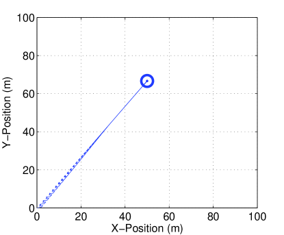
Figure 1: Trajectory of the agreements to the rendezvous point in x-y plane.

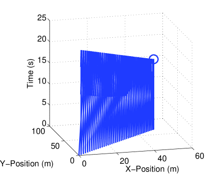
Figure 2: Trajectory of the agreements to the rendezvous with time.

Fig.3 and Fig.4 present the errors to the actual minimum time rendezvous point, $\left(50m,66m\right)$, during the procedure. In Fig.3 the Bregman’s projection is applied every time after the Dykstra’s projection proceeds 50 cycles, and in Fig.4 100 cycles. As the results shown, the frequency of Bregman’s projection applied not only affects the convergent rate but also the accuracy. This is due to the fact that reducing the frequency of Bregman’s projection means more Dykstra’s projection would be used, and more accuracy of the projection onto the intersection of the cones would be achieved. Conversely, Bregman’s projection will quickly approach the solution with a rough estimate.

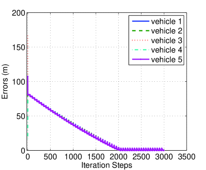
Figure 3: Error to the real minimum time rendezvous point with low frequency Bregman’s projection.

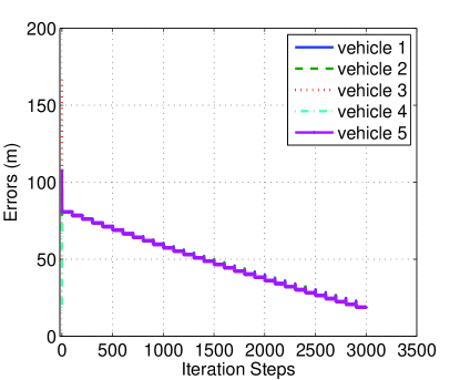
Figure 4: Error to the real minimum time rendezvous point with high frequency Bregman’s projection.

IV-B Scenario II: Asynchronous Bregman’s projecting

In this scenario, we let vehicle 1 reset its increment to zero every 50 cycles, vehicle 2 and 3 every 40 cycles, and vehicle 4 and 5 every 75 cycles. This setting will result in error on increments in the procedure of Dykstra’s projection.

As shown in Fig.5, the errors also converge to zero with around 2000 times interactions, about the same as the simultaneous case. Fig.6 illustrates the increment of time changes when the algorithm is applied. Although different frequency of reset is employed, the increments perform as if a global synchronous clock triggers Bregman’s projection. We speculate this as the result of nonlinear interactions within the vehicle.

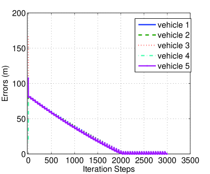
Figure 5: Error to the real minimum time rendezvous point with asynchronous Bregman s projecting.

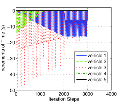
Figure 6: Increments of each vehicle when asynchronous Bregman s projecting applied.

V CONCLUSIONS AND FUTURE WORKS

We have proposed the distributed algorithm on multi-vehicle minimum time rendezvous point seeking which is composed of the Bregman’s and Dykstra’s alternating projection method. We have shown that the distance between the position plane and the intersection of the second-order cones is the minimum time for rendezvous, and the point on the plane that achieves the distance is the minimum time rendezvous point. The Bregman’s alternating projection was used to obtain the distance by consistent projections onto the plane and the intersection of the cones. Dykstra’s method guaranteed the vehicles with cyclic digraph interaction network had consensus on the projection of the point onto the intersection of the cones and only the communication with the neighbor is applied. The frequency of Bregman’s alternating projection applied to the vehicles ensures the converge speed, and the frequency of Dykstra’s alternating projection ensures the accuracy. The increments should be reset to zero after the procedure of cyclic Dykstra’s method, but the demonstration result showed that the vehicles could make the prediction on when to apply Bregman’s projection and reset the increment asynchronously. We believe the ability of asynchronous is linked to the characteristics of the alternating projection. This leaves the question of robustness of asynchronous open. In future research, we will analyze asynchronous character, and consider the interaction network with loose constraints.

VI ACKNOWLEDGMENTS

References

- [1] Y. Cao, W. Yu, W. Ren, and G. Chen, “An overview of recent progress in the study of distributed multi-agent coordination,” 2012.
- [2] W. Ren, R. W. Beard, and E. M. Atkins, “A survey of consensus problems in multi-agent coordination,” in American Control Conference, 2005. Proceedings of the 2005. IEEE, 2005, pp. 1859–1864.
- [3] E. Kranakis, D. Krizanc, and S. Rajsbaum, “Mobile agent rendezvous: A survey,” in Structural Information and Communication Complexity. Springer, 2006, pp. 1–9.
- [4] T. W. McLain, P. R. Chandler, S. Rasmussen, and M. Pachter, “Cooperative control of uav rendezvous,” in American Control Conference, 2001. Proceedings of the 2001, vol. 3. IEEE, 2001, pp. 2309–2314.
- [5] J. Lin, A. S. Morse, and B. D. Anderson, “The multi-agent rendezvous problem,” in Decision and Control, 2003. Proceedings. 42nd IEEE Conference on, vol. 2. IEEE, 2003, pp. 1508–1513.
- [6] J. Lin, A. S. Morse, and B. D. Anderson, “The multi-agent rendezvous problem-the asynchronous case,” in Decision and Control, 2004. CDC. 43rd IEEE Conference on, vol. 2. IEEE, 2004, pp. 1926–1931.
- [7] J. Cortés, S. Martínez, and F. Bullo, “Robust rendezvous for mobile autonomous agents via proximity graphs in arbitrary dimensions,” Automatic Control, IEEE Transactions on, vol. 51, no. 8, pp. 1289–1298, 2006.
- [8] J. Fang, A. S. Morse, and M. Cao, “Multi-agent rendezvousing with a finite set of candidate rendezvous points,” in American Control Conference, 2008. IEEE, 2008, pp. 765–770.
- [9] Q. Hui, “Finite-time rendezvous algorithms for mobile autonomous agents,” Automatic Control, IEEE Transactions on, vol. 56, no. 1, pp. 207–211, 2011.
- [10] P. Meschler, “Time-optimal rendezvous strategies,” Automatic Control, IEEE Transactions on, vol. 8, no. 4, pp. 279–283, 1963.
- [11] D. Chyung, “Time optimal rendezvous of three linear systems,” Journal of Optimization Theory and Applications, vol. 12, no. 3, pp. 242–247, 1973.
- [12] T. L. Brown, T. D. Aslam, and J. P. Schmiedeler, “Determination of minimum time rendezvous points for multiple mobile robots via level set methods,” in ASME 2011 International Design Engineering Technical Conferences and Computers and Information in Engineering Conference. American Society of Mechanical Engineers, 2011, pp. 787–797.
- [13] A. Bhatia and E. Frazzoli, “Decentralized algorithm for minimum-time rendezvous of dubins vehicles,” in American Control Conference, 2008. IEEE, 2008, pp. 1343–1349.
- [14] Y. J. Crispin, “Interception and rendezvous between autonomous vehicles,” Advances in Robotics, Automation and Control Vienna, Austria: InTech Publishing KG, 2008.
- [15] Y.-Z. Luo, G.-J. Tang, and H.-y. Li, “Optimization of multiple-impulse minimum-time rendezvous with impulse constraints using a hybrid genetic algorithm,” Aerospace science and technology, vol. 10, no. 6, pp. 534–540, 2006.
- [16] B. Paiewonsky and P. J. Woodrow, “Three-dimensional time-optimal rendezvous.” Journal of Spacecraft and Rockets, vol. 3, no. 11, pp. 1577–1584, 1966.
- [17] B. S. Burns, P. A. Blue, and M. D. Zollars, “Autonomous control for automated aerial refueling with minimum-time rendezvous,” in Proceedings of AIAA Guidance, Navigation and Control Conference, 2007.
- [18] D. B. Wilson, M. A. T. Soto, A. H. Goktogan, and S. Sukkarieh, “Real-time rendezvous point selection for a nonholonomic vehicle,” in Robotics and Automation (ICRA), 2013 IEEE International Conference on. IEEE, 2013, pp. 3941–3946.
- [19] G. Notarstefano and F. Bullo, “Distributed consensus on enclosing shapes and minimum time rendezvous,” in Decision and Control, 2006 45th IEEE Conference on. IEEE, 2006, pp. 4295–4300.
- [20] M. K. Tam, “The method of alternating projections,” Ph.D. dissertation, University of Newcastle, Australia, 2012.
- [21] P. L. Combettes and J.-C. Pesquet, “Proximal splitting methods in signal processing,” in Fixed-point algorithms for inverse problems in science and engineering. Springer, 2011, pp. 185–212.
- [22] S. Boyd and J. Dattorro, “Alternating projections,” Lecture notes of EE 392 o, Stanford University, Autumn Quarter, vol. 2004, 2003.
- [23] R. Escalante and M. Raydan, “Dykstra’s algorithm for a constrained least-squares matrix problem,” Numerical linear algebra with applications, vol. 3, no. 6, pp. 459–471, 1996.
- [24] S. Boyd, N. Parikh, E. Chu, B. Peleato, and J. Eckstein, “Distributed optimization and statistical learning via the alternating direction method of multipliers,” Foundations and Trends® in Machine Learning, vol. 3, no. 1, pp. 1–122, 2011.
- [25] S. P. Boyd and L. Vandenberghe, Convex optimization. Cambridge university press, 2004.