Energy-based Analysis of Biochemical Cycles using Bond Graphs

Abstract

Thermodynamic aspects of chemical reactions have a long history in the Physical Chemistry literature. In particular, biochemical cycles require a source of energy to function. However, although fundamental, the role of chemical potential and Gibb’s free energy in the analysis of biochemical systems is often overlooked leading to models which are physically impossible.

The bond graph approach was developed for modelling engineering systems where energy generation, storage and transmission are fundamental. The method focuses on how power flows between components and how energy is stored, transmitted or dissipated within components. Based on early ideas of network thermodynamics, we have applied this approach to biochemical systems to generate models which automatically obey the laws of thermodynamics. We illustrate the method with examples of biochemical cycles.

We have found that thermodynamically compliant models of simple biochemical cycles can easily be developed using this approach. In particular, both stoichiometric information and simulation models can be developed directly from the bond graph. Furthermore, model reduction and approximation while retaining structural and thermodynamic properties is facilitated. Because the bond graph approach is also modular and scaleable, we believe that it provides a secure foundation for building thermodynamically compliant models of large biochemical networks.

1 Introduction

Oh ye seekers after perpetual motion, how many vain chimeras have you pursued? Go and take your place with the alchemists. Leonardo da Vinci, 1494

Thermodynamic aspects of chemical reactions have a long history in the Physical Chemistry literature. In particular, the role of chemical potential and Gibb’s free energy in the analysis of biochemical systems is developed in, for example, the textbooks of Hill [1], Beard and Qian [2] and Keener and Sneyd [3]. As discussed by, for example, Katchalsky and Curran [4] and Cellier [5, Chapter 8], there is a distinction between classical thermodynamics which treats closed systems which are in equilibrium or undergoing reversible processes and non-equilibrium thermodynamics which treats systems, such as living organisms, which are open and irreversible.

Biochemical cycles are the building-blocks of biochemical systems; as discussed by Hill [1], they require a source of energy to function. For this reason, the modelling of biochemical cycles requires close attention to thermodynamical principles to avoid models which are physically impossible. Such physically impossible models are analogous to the perpetual motion machines beloved of inventors. In the context of biochemistry, irreversible reactions are not, in general, thermodynamically feasible and can be erroneously used to move chemical species against a chemical gradient thus generating energy from nothing [6]. The theme of this paper is that models of biochemical networks must obey the laws of thermodynamics; therefore it is highly desirable to specify a modelling framework in which compliance with thermodynamic principles is automatically satisfied. Bond graphs provide one such framework.

Bond graphs were introduced by Henry Paynter (see Paynter [7] for a history) as a method of representing and understanding complex multi-domain engineering systems such as hydroelectric power generation. A comprehensive account of bond graphs is given in the textbooks of Gawthrop and Smith [8], Borutzky [9] and Karnopp et al. [10] and a tutorial introduction for control engineers is given by Gawthrop and Bevan [11].

As discussed in the textbooks of, for example, Palsson [12, 13], Alon [14] and Klipp et al. [15], the numerous biochemical reactions occurring in cellular systems can be comprehended by arranging them into networks and analysing them by graph theory and using the associated connection matrices. These two aspects of biochemical reactions – thermodynamics and networks – were brought together some time ago by Oster et al. [16]. A comprehensive account of the resulting network thermodynamics is given by Oster et al. [17]. As discussed by Oster and Perelson [18] such thermodynamic networks can be analysed using an equivalent electrical circuit representation; but, more generally, the bond graph approach provides a natural representation for network thermodynamics [19, 20, 17]. This approach was not widely adopted by the biological and biochemical modelling community, and may be considered to have been ahead of its time. Mathematical modelling and computational analysis of biochemical systems has developed a great deal since then, and now underpins the new disciplines of systems biology [21], and “physiome” modelling of physiological systems [22, 23, 24, 25], where we are faced with the need for physically feasible models across spatial and temporal scales of biological organisation.

In particular there has been a resurgence of interest in this approach to modelling as it imposes extra constraints on models, reducing the space of possible model structures or solutions for consideration. This has been applied from individual enzymes [26, 27] and cellular pathways [28] up to large scale models [29, 30, 31], as a way of eliminating thermodynamically infeasible models of biochemical processes and energetically impossible solutions from large scale biochemical network models alike (see Soh and Hatzimanikatis [32] for a review). Additionally, there is new impetus into model sharing and reuse in the biochemical and physiome modelling communities which has garnered interest in modular representations of biochemical networks, and has promoted development of software, languages and standards and databases for models of biochemical processes. Model representation languages such as CellML and SBML promote model sharing through databases such as the Physiome Model Repository and BioModels Database. Descriptions of models in a hierarchical and modular format allows components of models to be stored in such databases and assembled into new models. Rather than to revisit the detailed theoretical development, therefore, our aim is therefore to refocus attention on the bond graph representation of biochemical networks for practical purposes such as these. First we briefly review the utility of the bond graph approach with these aims in mind.

Bond graph approaches have also developed considerably in recent years, in particular through the development of computational tools for their analysis, graphical construction and manipulation, and modularity and reuse [33, 34, 35, 36, 37, 38], which are key preoccupations for systems biology and physiome modelling. Our focus is on how kinetics and thermodynamic properties of biochemical reactions can be represented in this framework, and how the bond graph formalism allows key properties to be calculated from this representation. In addition, bond graph approaches have been extended in recent years to model electrochemical storage devices [39] and heat transfer in the context of chemical reactions [40]. Cellier [5] extends network thermodynamics beyond the isothermal, isobaric context of Oster et al. [17] by accounting for both work and heat and a series of papers [37, 41] shows how multi-bonds can be used to model the thermodynamics of chemical systems with heat and work transfer and convection and to simulate large systems. Thoma and Atlan [42] discuss “osmosis as chemical reaction through a membrane”. LeFèvre et al. [43] model cardiac muscle using the bond graph approach.

Bond graphs explicitly model the flow of energy through networks making use of the concept of power covariables: pairs of variable whose product is power. For example, in the case of electrical networks, the covariables are chosen as voltage and current. As discussed by a number of authors [1, 5, 44, 45], chemical potential is the driving force of chemical reactions. Hence, as discussed by Cellier [5], the appropriate choice of power covariables for isothermal, isobaric chemical reaction networks is chemical potential and molar flow rates. As pointed out by Beard et al. [30], using both mass and energy balance ensures that models of biochemical networks are thermodynamically feasible. Modelling using bond graphs automatically ensures not only mass-balance but also energy-balance; thus models of biochemical networks developed using bond graphs are thermodynamically feasible.

As discussed by Hill [1], biochemical cycles are the building-blocks of biochemical systems. Bond graph models are able to represent thermodynamic cycles and therefore appropriately represent free energy transduction in biochemical processes in living systems.

Living systems are complex, and therefore a hierarchical and modular approach to modelling biochemical systems is desirable. Bond graphs have a natural hierarchical representation [46] and have been used to model complex network thermodynamics [5, 37, 41]. Complex systems can be simplified by approximation: the bond graph method has a formal approach to approximation [8, 11, 10] and the potential algebraic issues arising from such approximation [47]. In particular, complex systems can be simplified if they exhibit a fast and slow timescale; a common feature of many biochemical (for example, Michaelis-Menten enzyme kinetics) and cell physiological systems (for example, slow-fast analysis of the membrane potential of electrically excitable cells). A bond graph approach to two-timescale approximation has been presented by Sueur and Dauphin-Tanguy [48].

As well as providing a thermodynamically-consistent model of a dynamical system suitable for simulation, representation of a biochemical system using the bond graph approach enables a wide range of properties and characteristics of the system to be represented. A number of key physical properties can be derived directly from the bond graph representation. For example, chemical reactions involve interactions between species which preserve matter; the number of moles of each species in a reaction must be accounted for.

As discussed by Oster et al. [17, §5.2], the kinetics of biochemical networks become particularly simple near thermodynamic equilibrium. However, as discussed by Qian and Beard [49], it is important to consider the behaviour of biochemical networks in living systems far from equilibrium. In particular, the analysis of non-equilibrium steady-states (where flows are constant but non-zero and states are constant) is important [50, 2].

Using elementary reactions as examples, §2 shows how biochemical networks may be modelled using bond graphs. The bond graph is more than a sketch of a biochemical network; it can be directly interpreted by a computer and, moreover, has a number of features that enable key physical properties to be derived from the bond graph itself. For example, §3 shows how the bond graph can be used to examine the stoichiometric properties of biochemical networks. §4 discusses the role of bond graphs in the structural approximation of biochemical networks. §5 discusses two biochemical cycles, an enzyme catalysed reaction and a biochemical switch, to illustrate the main points of the paper. §6 discusses software aspects of the Bond Graph approach and how it could be integrated into preexisting hierarchical modelling frameworks. §7 concludes the paper.

2 Bond Graph Modelling of Chemical Reactions

(a) $A{\;\xrightleftharpoons{}\;}B$

(b) $A{\;\xrightleftharpoons{}\;}B$

(c) $A{\;\xrightleftharpoons{1}\;}B{\;\xrightleftharpoons{2}\;}C$

(d) $A+B{\;\xrightleftharpoons{}\;}C+D$

(e) $A{\;\xrightleftharpoons{}\;}2B$

(f) $S+E{\;\xrightleftharpoons{}\;}P+E$

(g) $\xrightarrow{v}A{\;\xrightleftharpoons{1}\;}B{\;\xrightleftharpoons{2}\;}C\xrightarrow{v}$

(h) $A{\;\xrightleftharpoons{1}\;}B{\;\xrightleftharpoons{2}\;}C{\;\xrightleftharpoons{3}\;}D{\;\xrightleftharpoons{4}\;}A$

Figure 1: Simple reactions and their bond graphs. (a) The simple binary reaction is represented by a bond graph using a C component for each substance and an Re component to explicitly represent the reaction. (b) An alternative representation using 0 (common potential) junctions to allow connections. (c) Two reactions in series extending (b). (d) A single reaction between four substances requires a single Re component, one C component for each substance and two 1 (common flow) connections. (e) The stoichiometric coefficient $2$ can be incorporated using the bond graph TF  component. (f) A simple enzyme-catalysed reaction. The enzyme $E$ appears on each side of the formula thus creating a cycle in the bond graph (see §55.1). (g) The same as (c) but with an externally-imposed flow that adds molecules of $A$ whilst subtracting the same number of molecules of $C$ thus allowing a non-equilibrium steady-state. (h) A simple biochemical cycle.

Bond graphs are an energy-based modelling approach. This section introduces the bond graph methodology in the context of biochemical reactions using the reactions listed in figure 1. The section is organised to emphasise the key aspects of bond graph modelling which make it a powerful approach to the modelling of biochemical systems.

2.1 Energy flow, storage and dissipation in a simple reversible reaction

figure 1(a) shows the simple interconversion of two molecular species, A and B. As mentioned above, a thermodynamically consistent representation of biochemical processes demands consideration of reversible reactions, and so we consider this simple interconversion as the simplest possible reaction. This interconversion is represented by bonds of the form each of which is associated with two variables: the chemical potential $\mu$ $(\text{J mol}^{-1})$ and a molar flow rate $v$ $(\text{mol s}^{-1})$. The product of these two variables is energy flow or power $P=\mu\times v$ $(\text{W})$. The bonds represent the transmission of power in the system, and do not not create, store or dissipate power. The half-arrow on the bond indicates the direction in which power flow will be regarded as positive and thus defines a sign convention.

In figure 1(a) the pools of chemical species A and B are represented by C components. These components reflect the amount of each species present (and hence determine the chemical potential of each species). C:$\mathbf{A}$ contains $x_{a}$ moles of species $A$ and the rate of decrease is equal to the molar flow $v$; C:$\mathbf{B}$ contains $x_{b}$ moles of species $B$ and the rate of increase is $v$. Thus:

$$\dot{x}_{a} =-v \dot{x}_{b} =v$$ (1)

Each C component is associated with a chemical potential $\mu$ which, assuming a dilute system within a volume $V$, is given by [3, §1.2]:

$$\mu_{a} =\mu_{a}^{0}+RT\ln\frac{x_{a}}{V} \mu_{b} =\mu_{b}^{0}+RT\ln\frac{x_{b}}{V}$$ (2)

where $\mu_{a}^{0}$ is the standard chemical potential for species A, and similarly for species B. It is convenient to rewrite Equations (2) as:

$$\mu_{a} =RT\ln K_{a}x_{a} \mu_{b} =RT\ln K_{b}x_{b} \text{where }K_{a} =\frac{1}{V}e^{\frac{\mu_{a}^{0}}{RT}} \text{and }K_{b} =\frac{1}{V}e^{\frac{\mu_{b}^{0}}{RT}}$$ (3)

Each C component stores but does not create or dissipate energy. The corresponding energy flow is described through the bond to which it is connected.

The reversible reaction between chemical species $A$ and $B$ is represented by a single Re (Reaction) component which relates the reaction flow $v$ to the chemical affinities (weighted sum of chemical potentials) for the forwards and reverse reactions $A^{f}=\mu_{a}$ and $A^{r}=\mu_{b}$. As discussed by Van Rysselberghe [51] and Oster et al. [17, §5.1], the reaction rate, or molar flow, is given by the Marcelin – de Donder formula:

$$v =v^{+}-v^{-} \text{where }v^{+} =\kappa e^{\frac{A^{f}}{RT}} \text{and }v^{-} =\kappa e^{\frac{A^{r}}{RT}}$$ (4)

where $\kappa$ is a constant which determines reaction rate. This can be rewritten in two ways. The de Donder formula [52, Equation(11)]:

$$\frac{v^{+}}{v^{-}} =e^{\frac{A}{RT}} \text{where }A =A^{f}-A^{r}$$ (5)

and the Marcelin formula [53, Equation(1)]:

$$v=\kappa\left(e^{\frac{A^{f}}{RT}}-e^{\frac{A^{r}}{RT}}\right)$$ (6)

This latter formulation is used in the sequel. The Re component dissipates, but does not create or store, energy.

In the particular case of figure 1(a), substituting the chemical potentials of Equations (3) into Equations (4) recovers the well known first-order mass-action expressions:

$$v^{+} =\kappa K_{a}x_{a} v^{-} =\kappa K_{b}x_{b} v =\kappa\left(K_{a}x_{a}-K_{b}x_{b}\right)$$ (7)

We note that this notation clearly demarcates parameters relating to thermodynamic quantities ($K_{a},K_{b}$) from reaction kinetics ($\kappa$) and that the equilibrium constant is given by $K_{b}/K_{a}$.

The Equations (7) can also be written in the conventional rate constant form as

$$v^{+} =k^{+}x_{a} v^{-} =k^{-}x_{b} v =v^{+}-v^{-}=k^{+}x_{a}-k^{-}x_{b}$$ (8)

where the forwards and backwards first order rate constants are

$$k^{+}=\kappa K_{a}\text{ and }k^{-}=\kappa K_{b}$$ (9)

The thermodynamic quantities and reaction kinetics are no longer distinguished in the rate constant formulation of Equations (8).

2.2 Modularity: coupling reactions into networks

A key feature of bond graph representations is to construct and analyse models of large scale systems from simpler building blocks. The bond graph of figure 1(a) cannot be used as a building block of a larger system as there are no connections available with which to couple to other reactions. However, the bond graph approach is, in general, modular and provides two connection components for this purpose: the 0 junction and the 1 junction. Each of these components transmits, but does not store, create or dissipate energy. In figure 1(b) the representation of the simple reversible reaction in figure 1(a) is expanded to include two 0 junction connectors. This representation is identical to that in figure 1(a) except that it makes explicit the junctions through which other reactions involving species A and B can be coupled to this reaction. The bond graph of figure 1(c) makes use of the right-hand 0 junction of figure 1(b) to build two connected reactions; where species B is also reversibly interconverts with species C.

The connector in this case is a 0 junction. The 0 junction can have two or more impinging bonds. In the case of the central 0 junction of figure 1(c), there are three impinging bonds: one () pointing in and two ( and ) pointing out. As indicated in figure 1(c), the 0 junction has two properties:

1. the chemical potentials or affinities (efforts) on all impinging bonds are constrained to be the same, (the 0 junction is therefore a common potential connector), and

2. the molar flows on the impinging bonds sum to zero, under the sign convention that a plus sign is appended to the flows corresponding to inward bonds and a minus sign for outward bonds:

   $$v_{1}-v_{b}-v_{2} =0 \text{or }v_{b} =v_{1}-v_{2}$$ (10)

These two properties imply a third: the power flowing out of a 0 junction is equal to the power flowing in (the 0 junction is power-conserving):

$$P_{a}+P_{2}=\mu_{b}v_{b}+\mu_{b}v_{2}=\mu_{b}(v_{b}+v_{2})=\mu_{b}v_{1}=P_{1}$$ (11)

In a similar fashion, the left-hand 0 junction implies that $v_{a}=-v_{1}$ and the right-hand 0 junction implies that $v_{c}=v_{2}$. Figure 1(c) can easily be extended to give a reaction chain of arbitrary length.

In contrast, in order to represent the reaction of figure 1(d) we introduce the 1 junction, which has the same power-conserving property as the 0 junction but which represents a common flow connector. In particular, with reference to the left-hand 1 junction in figure 1(d):

1. the molar flows on all impinging bonds are constrained to be the same and

2. the affinities on the impinging bonds sum to zero when a plus sign is appended to the efforts corresponding to inward bonds and a minus sign for outward bonds:

   $$\mu_{a}+\mu_{b}-A^{f} =0 \text{or }A^{f} =\mu_{a}+\mu_{b}$$ (12)

Similarly, the right-hand 1 junction implies that:

$$A^{r}-\mu_{c}-\mu_{d} =0 \text{or }A^{r} =\mu_{c}+\mu_{d}$$ (13)

substituting the chemical potentials of Equations (12) and (13) into Equations (4) gives the well known second-order mass-action expression:

$$v =\kappa\left(K_{a}x_{a}K_{b}x_{b}-K_{c}x_{c}K_{d}x_{e}\right)=k^{+}x_{a}x_{b}-k^{-}x_{c}x_{d}$$ (14)

$$\text{where }k^{+} =\kappa K_{a}K_{b}\text{ and }k^{-}=\kappa K_{c}K_{d}$$ (15)

Once again, we note that this notation clearly demarcates parameters relating to thermodynamic quantities ($K_{a},K_{b},K_{c},K_{d}$) from reaction kinetics ($\kappa$).

2.3 Incorporating stoichiometry into reactions

The reaction of figure 1(e) has one mole of species $A$ reacting to form two moles of species $B$. The corresponding bond graph uses the TF component to represent this stoichiometry. The TF component transmits, but does not store, create or dissipate energy. Hence, the power out equals the power in. Thus in the context of figure 1(e):

$$A^{r}v=\mu_{b}v_{b}$$ (16)

(noting that in this case $A^{r}$ is the ‘unknown’ as $\mu_{b}$ is determined by the 0 junction).

A TF component with ratio $n$ is donated by TF:$\mathbf{n}$ and is defined by the power conserving property and that the output flow is $n$ times the input flow. As power is conserved, it follows therefore that the input effort is $n$ times the output effort. In the context of figure 1(e):

$$A^{r} =2\mu_{b} v_{b} =2v$$ (17)

Noting that $A_{f}=\mu_{a}$ it follows from Equations (4) that:

$$v =\kappa\left(K_{a}x_{a}-(K_{b}x_{b})^{2}\right)=k^{+}x_{a}-k^{-}x_{b}^{2}\text{ where }k^{+}=\kappa K_{a}\text{ and }k^{-}=\kappa K_{b}^{2}$$ (18)

2.4 Non-equilibrium steady states: reactions with external flows.

As has been discussed by many authors, in cells biochemical reactions are maintained away from thermodynamic equilibrium through continual mass and energy flow through the reaction. The reaction of figure 1(g) corresponds to the reaction in Figure 1(c) except that an external flow $v_{0}>0$ has been included. This corresponds to adding molecules of $A$ and removing molecules of $C$ at the same fixed rate. As discussed by Qian et al. [50], the reaction has a non-equilibrium steady-state (NESS) corresponding to $v_{1}=v_{2}=v_{0}$. This is a steady-state because the flows $v_{a}=v_{b}=v_{c}=0$ and hence $\dot{x}_{a}=\dot{x}_{b}=\dot{x}_{c}=0$; it is not a thermodynamic equilibrium because $v_{1}\neq 0$ and $v_{2}\neq 0$.

2.5 Thermodynamic compliance

The bond graph approach ensures thermodynamic compliance: the model may not be correct, but it does obey the laws of thermodynamics. To illustrate this point, consider the Biochemical Cycle of figure 1(h). As discussed by, for example, Qian et al. [50], a fundamental property of such cycles is the thermodynamic constraint that

$$\frac{k_{+1}k_{+2}k_{+3}k_{+4}}{k_{-1}k_{-2}k_{-3}k_{-4}}=1$$ (19)

This property arises from the requirement for detailed balance around the biochemical cycle. However, as is now shown, the thermodynamic constraint of Equation (19) is automatically satisfied by the bond graph representation of figure 1(h).

In the same way as Equation (8), the four reaction flows can be written as:

$$v_{1} =\kappa_{1}\left(K_{a}x_{a}-K_{b}x_{b}\right), \dots, v_{4} =\kappa_{4}\left(K_{d}x_{d}-K_{a}x_{a}\right)$$ (20)

Alternatively, the four reaction flows of Equations (20) can be rewritten as:

$$v_{1} =\left(k_{+1}x_{a}-k_{-1}x_{b}\right), \dots, v_{4} =\left(k_{+4}x_{d}-k_{-4}x_{a}\right)$$ (21)

where

$$k_{+1} =\kappa_{1}K_{a}, \dots, k_{+4} =\kappa_{4}K_{d}, k_{-1} =\kappa_{1}K_{b}, \dots, k_{-4} =\kappa_{4}K_{a}$$ (22)

Hence:

$$\frac{k_{+1}k_{+2}k_{+3}k_{+4}}{k_{-1}k_{-2}k_{-3}k_{-4}}=\frac{\kappa_{1}K_{a}\kappa_{2}K_{b}\kappa_{3}K_{c}\kappa_{4}K_{d}}{\kappa_{1}K_{b}\kappa_{2}K_{c}\kappa_{3}K_{d}\kappa_{4}K_{a}}$$ (23)

As each factor of the numerator on the right-hand side of Equation (23) appears in the denominator, and vice versa, then Equation (19) is satisfied.

3 Stoichiometric Analysis of Reaction Networks

Stoichiometric analysis is fundamental to understanding the properties of large networks [12, 13, 54]. In particular computing the left and right null space matrices leads to information about pools and steady-state pathways [55, 56, 57, 58]. For example, when analysing reaction networks such as metabolic networks, one may seek to determine for measured rates of change of metabolite concentrations, what are the reaction rates in the network. This question is addressed below. Initially we will address the inverse problem: for given reaction velocities, what are the rates of change of concentrations of the chemical species? In bond graph terms, this asks the question: “given the reaction flows $V$, what are the flows $\dot{X}$ at the C components?”. This can be addressed directly from the bond graph using the concept of causality.

The bond graph concept of causality [8, 11, 10] has proved useful for generating simulation code, detecting modelling inconsistencies, solving algebraic loops [47], approximation, inversion [59, 60, 61] and analysis of system properties [62]. This section shows how the bond graph concept of causality can be used to examine the stoichiometry of networks of biochemical reactions. As in §2, this is done by analysis of particular examples. However, as discussed in Section 6, this approach scales up to arbitrarily large systems.

3.1 The stoichiometric matrix

(a) $A{\;\xrightleftharpoons{}\;}B$

(b) $A{\;\xrightleftharpoons{1}\;}B{\;\xrightleftharpoons{2}\;}C$

(c) $A+B{\;\xrightleftharpoons{}\;}C+D$

(d) $\xrightarrow{v_{0}}A{\;\xrightleftharpoons{1}\;}B{\;\xrightleftharpoons{2}\;}C\xrightarrow{v_{0}}$

Figure 2: Causal strokes and the Stoichiometric Matrix. The bond graph notion of causality provides an algorithm for determining the stoichiometric matrix by explicitly showing how the Re flows propagate to the C flows. (a) The C components impose a potential onto the Re component; the Re component imposes a flow into the C components. (b) As (a) and note that exactly one bond imposes a potential on to each 0 (common potential) junction. (c) As (a) and note that exactly one bond imposes a flow on to each 1 (common flow) junction. (d) As the external flow $v_{0}$ impinges on to 0 junctions, it does not affect the causality of the parts in common with (b).

Figure 2(a) is similar to the bond graph of figure 1(a) except that two lines have been added perpendicular to each bond; these lines are called causal strokes. It is convenient to distinguish between the flows on each side of the Re component by relabelling them as $v^{f}$ and $v^{r}$ ($v^{f}=v_{r}=v$) and this is reflected in the annotation. The implications of the causal stroke are twofold:

1. The bond imposes effort on the component at the stroke end of the bond.

2. The bond imposes flow on the component at the other end of the bond.

Thus, as indicated on the bond graph: the flows are given by:

$$\dot{x}_{a} =-v_{a}=-v^{f}=-v \dot{x}_{b} =v_{b}=v^{r}=v$$ (24)

and the efforts by

$$A_{f} =\mu_{a} A_{r} =\mu_{b}$$ (25)

In general, the reaction flows can be composed into the vector $V$, and the state derivatives into the vector $X$, and these are related by the stoichiometric matrix $N$:

$$\dot{X} =NV$$ (26)

In the case of figure 2(a):

$$X =\begin{pmatrix}x_{a}\\ x_{b}\end{pmatrix} V =v \text{and }N=\begin{pmatrix}-1\\ 1\end{pmatrix}$$ (27)

The system of figure 2(b) has 3 C components and the state $X$ can be chosen as:

$$X=\begin{pmatrix}x_{a}&x_{b}&x_{c}\end{pmatrix}^{T}$$ (28)

There are two reaction flows $v_{1}$ and $v_{2}$ corresponding to Re:$\mathbf{1}$ and Re:$\mathbf{2}$ respectively. The flow vector $V$ can be chosen as:

$$V=\begin{pmatrix}v_{1}&v_{2}\end{pmatrix}^{T}$$ (29)

Following the causal strokes and observing the sign convention at the 0 junction:

$$\dot{x}_{a} =v_{a}=-v_{1} \dot{x}_{b} =v_{b}=v_{1}-v_{2} \dot{x}_{c} =v_{c}=v_{2}$$ (30)

Using (28) and (29), it follows that:

$$\dot{X} =NV \text{where }N =\begin{pmatrix}-1&0\\ 1&-1\\ 0&1\end{pmatrix}$$

The system of figure 2(d) is the same as that of figure 2(b) but with an additional input $v_{0}$ and so $V$ is defined as:

$$V=\begin{pmatrix}v_{0}&v_{1}&v_{2}\end{pmatrix}^{T}$$ (31)

Using the summing rules at the left and right 0 junctions, it follows that:

$$\dot{X} =NV \text{where }N =\begin{pmatrix}1&-1&0\\ 0&1&-1\\ -1&0&1\end{pmatrix}$$

The system of figure 2(c) has 4 C components and the state $X$ can be chosen as:

$$X=\begin{pmatrix}x_{a}&x_{b}&x_{c}&x_{d}\end{pmatrix}^{T}$$ (32)

There is one reaction flows $v$ corresponding to Re . The flow vector $V$ is thus scalar in this case:

$$V=v$$ (33)

Following the causal strokes and observing the sign convention at the 0 junction:

$$\dot{x}_{a} =v_{a}=-v \dot{x}_{b} =v_{b}=-v \dot{x}_{c} =v_{c}=v \dot{x}_{d} =v_{d}=v$$ (34)

Using (28) and (29), it follows that:

$$\dot{X} =NV$$

$$\text{where }N =\begin{pmatrix}-1&-1&1&1\end{pmatrix}^{T}$$ (35)

In bond graph terms this particular arrangement of causal strokes is known as integral causality. Naturally this analysis extends to arbitrarily large systems, and can be carried out algorithmically in automated software.

3.2 Stoichiometric null spaces

(a) $A{\;\xrightleftharpoons{}\;}B$

(b) $A{\;\xrightleftharpoons{1}\;}B{\;\xrightleftharpoons{2}\;}C$

(c) $A+B{\;\xrightleftharpoons{}\;}C+D$

(d) $\xrightarrow{v_{0}}A{\;\xrightleftharpoons{1}\;}B{\;\xrightleftharpoons{2}\;}C\xrightarrow{v_{0}}$

Figure 3: Causal strokes and the Stoichiometric Matrix Subspaces. The bond graph notion of causality provides an algorithm for determining the subspaces of the stoichiometric matrix by explicitly showing how the C flows propagate to other C flows and and to the Re flows. (a) C:$\mathbf{A}$ imposes a flow into Re which in turn imposes a flow into C:$\mathbf{B}$. (b) C:$\mathbf{A}$ imposes a flow into Re:$\mathbf{1}$ and thence, together with C:$\mathbf{B}$. imposes a flow into the 0 junction and thence into Re:$\mathbf{2}$ and C:$\mathbf{C}$. (c) C:$\mathbf{A}$ imposes a flow into the 1 junction and thence into C:$\mathbf{B}$ and Re ; Re in turn imposes a flow into the 1 junction and thence into C:$\mathbf{C}$ and C:$\mathbf{D}$. (d) As the external flow $v_{0}$ impinges on to 0 junctions, it does not affect the causality of the parts in common with (b).

The causal analysis of §3.1 asks the question: “given the reaction flows $V$, what are the flows $\dot{X}$ at the C components?”. This section looks at the inverse question: “given the flows $\dot{X}$ at the C components, what are the reaction flows $V$?”

With this in mind, the causal stroke on the bond impinging on the C:$\mathbf{A}$ component in figure 3(a) is now at the C end of the bond, thus imposing flow on the Re component and so $v^{f}=v_{a}$. There is now a causal issue: as $v_{r}=v_{f}$, it follows that $v_{r}$ is also determined by the C:$\mathbf{A}$ component and $v_{r}=v_{a}$. Hence the flow on the bond impinging on C:$\mathbf{B}$ is determined and the causality must be as shown. Thus causal considerations show that the flow $v_{a}$ determines the flow $v_{b}$ which therefore cannot be independently chosen. In bond graph terms this particular arrangement of causal strokes is known as derivative causality. To summarise:

$$v =v_{a}=-\dot{x}_{a} \dot{x}_{b} =v=-\dot{x}_{a}$$ (36)

The system of figure 3(a) has 2 C components and

$$X=\begin{pmatrix}x_{a}&x_{b}\end{pmatrix}^{T}$$ (37)

It is convenient to decompose $X$ into two components: $x$ the independent part of $X$ and $X^{d}$ the dependent part of $X$. In particular:

$$x =x_{a}=L_{xX}X\text{ where }L_{xX}=\begin{pmatrix}1&0\end{pmatrix}$$ (38)

$$\text{ and }X^{d} =\begin{pmatrix}x_{b}\end{pmatrix}=L_{dX}X\text{ where }L_{dX}=\begin{pmatrix}0&1\end{pmatrix}$$ (39)

The full state $X$ can be reconstructed from $x$ and $X^{d}$ using:

$$X=L_{xX}^{T}x+L_{dX}^{T}X^{d}$$ (40)

Using this decomposition Equations (36) can be written as:

$$\dot{X}^{d} =L_{dx}\dot{x}$$ (41)

$$\text{where }L_{dx} =\begin{pmatrix}-1\end{pmatrix}$$ (42)

Combining these equations,

$$\dot{X}^{d}=L_{dX}\dot{X}=L_{dx}\dot{x}=L_{dx}L_{xX}\dot{X}$$ (43)

Defining

$$G=L_{dX}-L_{dx}L_{xX}$$ (44)

it follows that the state dependency can also be expressed as:

$$G\dot{X}=GNV=0$$ (45)

where, in this case:

$$G =\begin{pmatrix}0&1\end{pmatrix}+\begin{pmatrix}1&0\end{pmatrix}=\begin{pmatrix}1&1\end{pmatrix}$$ (46)

As discussed in the textbooks, as (45) is true for all $V$,

$$GN=0$$ (47)

and thus $G$ is a left null matrix of $N$. In this particular case $G\dot{X}=0$ corresponds to:

$$\dot{x}_{a}+\dot{x}_{b} =0$$ (48)

$$\text{or }x_{a}+x_{b} =\text{const}$$

Thus the total amount of $A$ and $B$ is constant.

The system of figure 3(b) has 3 C components and

$$X=\begin{pmatrix}x_{a}&x_{b}&x_{c}\end{pmatrix}^{T}$$ (49)

Following the same arguments as for figure 3(a), it follows that:

$$x =\begin{pmatrix}x_{a}\\ x_{b}\end{pmatrix}=L_{xX}X\text{where }L_{xX}=\begin{pmatrix}1&0&0\\ 0&1&0\end{pmatrix}$$ (50)

$$\text{and }X^{d} =\begin{pmatrix}x_{c}\end{pmatrix}=L_{dX}X\text{ where }L_{dX}=\begin{pmatrix}0&0&1\end{pmatrix}\text{ and }L_{dx}=\begin{pmatrix}-1&-1\end{pmatrix}$$ (51)

In this case:

$$G =L_{dX}-L_{dx}L_{xX}=\begin{pmatrix}0&0&1\end{pmatrix}-\begin{pmatrix}-1&-1\end{pmatrix}\begin{pmatrix}1&0&0\\ 0&1&0\end{pmatrix}=\begin{pmatrix}1&1&1\end{pmatrix}$$ (52)

In this particular case $G\dot{X}=0$ corresponds to:

$$\dot{x}_{a}+\dot{x}_{b}+\dot{x}_{c} =0$$ (53)

$$\text{or }x_{a}+x_{b}+x_{c} =\text{const}$$

Thus the total amount of $A$, $B$ and $C$ is constant.

The system of figure 3(c) has 4 C components and

$$X=\begin{pmatrix}x_{a}&x_{b}&x_{c}&x_{d}\end{pmatrix}^{T}$$ (54)

Following the same arguments as for figure 3(a), it follows that:

$$x =\begin{pmatrix}x_{a}\end{pmatrix}=L_{xX}X\text{ where }L_{xX}=\begin{pmatrix}1&0&0&0\end{pmatrix}$$ (55)

$$\text{and }X^{d} =\begin{pmatrix}x_{b}&x_{c}&x_{d}\end{pmatrix}^{T}=L_{dX}X$$ (56)

$$\text{where }L_{dX} =\begin{pmatrix}0&1&0&0\\ 0&0&1&0\\ 0&0&0&1\ \end{pmatrix}\text{ and }L_{dx}=\begin{pmatrix}1\\ -1\\ -1\end{pmatrix}$$ (57)

In this case:

$$G =L_{dX}-L_{dx}L_{xX}=\begin{pmatrix}0&1&0&0\\ 0&0&1&0\\ 0&0&0&1\ \end{pmatrix}-\begin{pmatrix}1\\ -1\\ -1\end{pmatrix}\begin{pmatrix}1&0&0&0\end{pmatrix}=\begin{pmatrix}-1&1&0&0\\ 1&0&1&0\\ 1&0&0&1\end{pmatrix}$$ (58)

In this particular case, $G\dot{X}=0$ corresponds to:

$$x_{b} =x_{a}+\text{const} x_{a}+x_{c} =\text{const} x_{a}+x_{d} =\text{const}$$

Thus the amount of $B$ equals the amount of $A$ plus a constant, the total amount of $A$ and $C$ is constant and the total amount of $A$ and $D$ is constant.

Continuing the analysis of the system of figure 3(b) but including the extra input of figure 3(d), the flow vector has an extra component $v_{0}$ and can be defined as:

$$V=\begin{pmatrix}v_{0}&v_{1}&v_{2}\end{pmatrix}^{T}$$ (59)

where $v_{1}$ and $v_{2}$ are the two reaction flows. It is convenient to decompose $V$ into two components: $v$ the independent part of $V$ and $V^{d}$ part of $V$ dependent on $\dot{X}$ and $v$. In particular:

$$v =v_{0}=K_{vV}V\text{ where }K_{vV}=\begin{pmatrix}1&0&0\end{pmatrix}$$ (60)

$$V^{d} =\begin{pmatrix}v_{1}\\ v_{2}\end{pmatrix}=K_{dV}V\text{ where }K_{dV}=\begin{pmatrix}0&1&0\\ 0&0&1\end{pmatrix}$$ (61)

Moreover, following the causal strokes in figure 3(d) the flow vector $V$ can be written in terms of the state derivative $\dot{X}$ and the independent flow $v$ as:

$$V =K_{VX}\dot{X}+K_{Vv}v$$ (62)

$$\text{where }K_{VX} =\begin{pmatrix}0&0&0\\ -1&0&0\\ -1&-1&0\end{pmatrix}\text{ and }K_{Vv}=\begin{pmatrix}1\\ 1\\ 1\end{pmatrix}$$ (63)

In the particular case that the system is in a steady state and so $\dot{X}=0$:

$$V =Kv\text{ where }K=K_{Vv}$$ (64)

Substituting into Equation (26) it follows that $NKv=0$. As this must be true for all $v$, it follows that $NK=0$ and thus $K$ is a right null matrix of $N$.

3.3 Reduced-order equations

The stoichiometric analysis of §§3.1 and 3.2 has many uses; one of these, reducing the order of the ODEs describing a system, is given here. Reducing system order gives a smaller set of equations to solve and may avoid numerical problems, for example arising from failure to recognise conserved moieties in a reaction system.

From Equation (41), the derivatives $\dot{X}^{d}$ of the dependent state $X^{d}$ can be written as linear transformation of the derivatives $\dot{x}$ of the independent state $x$ as:

$$\dot{X}^{d}=L_{dx}\dot{x}$$ (65)

Integrating this equation gives:

$$X^{d}-X^{d}(0)=L_{dx}(x-x(0))$$ (66)

where $X^{d}(0)$ and $x(0)$ are the values of $X^{d}$ and $x$ at time zero. Using Equations 38, 39 and (44), Equation (66) can be rewritten as:

$$X^{d} =L_{dx}x+X^{d}(0)-L_{dx}x(0)=L_{dx}x+(L_{dX}-L_{dx}L_{xX})X(0)=L_{dx}x+GX(0)$$ (67)

Using Equation (40) to reconstruct $X$ from $X^{d}$ given by Equation (67) and $x$ gives:

$$X =\left(L_{xX}^{T}+L_{dX}^{T}L_{dx}\right)x+L_{dX}^{T}GX(0)=Lx+G_{X}X(0)$$ (68)

$$\text{where }L =L_{xX}^{T}+L_{dX}^{T}L_{dx}\text{ and }G_{X}=L_{dX}^{T}G$$ (69)

Equation (67) gives an explicit expression for reconstructing the full state $X$ from the independent state $x$ and the initial state $X(0)$.

From Equation (26) the state $X$ is given by the system ODE as:

$$\dot{X}=NV(X,u)$$ (70)

where $u$ represents external flows (for example $v$ in figure 3 (d)). Using Equations (38) and (68), the ODE in $X$ of Equation (70) can be rewritten as the reduced order ODE in $x$ as:

$$\dot{x}=L_{xX}NV(Lx+G_{X}X(0),u)$$ (71)

and the full state reconstructed using Equation (68).

4 Model Reduction and Approximation of Reaction Mechanisms

As discussed in the introduction, complex systems can be simplified by approximation. However, it is crucial that such approximation does not destroy the compliance with thermodynamic principles reflected in the original system.

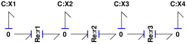
(a) Full system

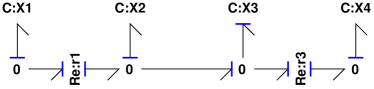
(b) Approximate system

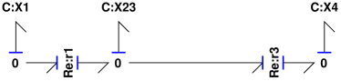
(c) Equivalent approximate system

Figure 4: Approximation of unimolecular reactions [26, §3.1]. The reaction chain (a) is approximated in (b) by assuming that the reaction represented by Re:$\mathbf{r2}$ is fast ($1/\kappa_{2}\approx 0$) and so may be removed. (c) is exactly equivalent to (b) except that the adjacent C:$\mathbf{X2}$ and C:$\mathbf{X3}$ are replaced by the composite component C:$\mathbf{X23}$ with coefficient $K_{23}$ given by Equation (83)

In their analysis of the Sodium Pump, which transports sodium ions out of electrically excitable cells such as cardiomyocytes, Smith and Crampin [26] consider simplification of the linear chain of reactions:

$$\cdots X_{1}{\;\xrightleftharpoons[k_{1}^{-}]{k_{1}^{+}}\;}X_{2}{\;\xrightleftharpoons[k_{2}^{-}]{k_{2}^{+}}\;}X_{3}{\;\xrightleftharpoons[k_{3}^{-}]{k_{3}^{+}}\;}X_{4}\cdots$$ (72)

where the middle reaction in the chain is fast relative to the other reactions. The three reactions have flows $v_{1}\dots v_{3}$ given by:

$$v_{1} =k_{1}^{+}X_{1}-k_{1}^{-}X_{2} v_{2} =k_{2}^{+}X_{2}-k_{2}^{-}X_{3} v_{3} =k_{3}^{+}X_{3}-k_{3}^{-}X_{4}$$ (73)

Reaction (72) corresponds to the bond graph of figure 4(a) which has the flows of Equations (73) where:

$$k_{1}^{+} =\kappa_{1}K_{1} k_{1}^{-} =\kappa_{1}K_{2}$$ (74)

$$k_{2}^{+} =\kappa_{2}K_{2} k_{2}^{-} =\kappa_{2}K_{3}$$ (75)

$$k_{3}^{+} =\kappa_{3}K_{3} k_{3}^{-} =\kappa_{3}K_{4}$$ (76)

If $\kappa_{2}\gg\kappa_{1}$ and $\kappa_{2}\gg\kappa_{3}$ Equation (75) can be rewritten as:

$$\kappa_{2}=\frac{1}{\epsilon}$$ (77)

where $\epsilon$ is a small positive number. $v_{2}$ (73) and (75) can then be rewritten as:

$$\epsilon v_{2}=K_{2}X_{2}-K_{3}X_{3}$$ (78)

assuming non-zero $v_{2}$ this means that as $\epsilon\rightarrow 0$, $X_{2}$ and $X_{3}$ are in equilibrium and:

$$X_{3} =\rho X_{2}\text{ where }\rho=\frac{K_{2}}{K_{3}}$$ (79)

This also means that the difference in affinities associated with reaction 2 is zero:

$$A^{f}_{2}-A^{r}_{2}=K_{2}X_{2}-K_{3}X_{3}=0$$ (80)

Thus the corresponding reaction component Re:$\mathbf{r3}$ can be removed from the bond graph to give figure 4(b). This implies that the C:$\mathbf{X3}$ component is in derivative causality and thus the bond graph represents a differential-algebraic equation and an ordinary differential equation. However, as discussed by Gawthrop and Bevan [11], as C:$\mathbf{X2}$ and C:$\mathbf{X3}$ are on adjacent 0 junctions, they may be replaced by the single C:$\mathbf{X23}$ component as in figure 4(c).

Figure 4(c) represents the same system as figure 4(b) if C:$\mathbf{X23}$ contains the same molar mass as C:$\mathbf{X2}$ and C:$\mathbf{X3}$. Moreover, using Equations (79)

$$X_{23}=X_{2}+X_{3}=(1+\rho)X_{2}$$ (81)

The equilibrium constant $K_{23}$ of C:$\mathbf{X23}$ must also correspond to those of C:$\mathbf{X2}$ and C:$\mathbf{X3}$ so that:

$$K_{2}X_{2} =K_{3}X_{3}=K_{23}X_{23}$$ (82)

$$\text{hence }K_{23} =\frac{K_{2}}{1+\rho}=\frac{\rho K_{3}}{1+\rho}$$ (83)

The bond graph of figure 4(c) corresponds to the reaction scheme [26, §3.1]:

$$\cdots X_{1}\overset{\alpha_{1}^{+}}{\underset{\alpha_{1}^{-}}{\rightleftharpoons}}X_{23}\overset{\alpha_{3}^{+}}{\underset{\alpha_{3}^{-}}{\rightleftharpoons}}X_{4}\cdots$$ (84)

where

$$\alpha_{1}^{+} =\kappa_{1}K_{1}=k_{1}^{+} \alpha_{1}^{-} =\kappa_{1}K_{23}=\kappa_{1}\frac{K_{2}}{1+\rho}=\frac{k_{1}^{-}}{1+\rho}$$

$$\alpha_{3}^{+} =\kappa_{3}K_{23}=\kappa_{1}\frac{\rho K_{3}}{1+\rho}=\frac{\rho k_{3}^{+}}{1+\rho}=\frac{k_{3}^{+}}{1+\frac{1}{\rho}} \alpha_{3}^{-} =\kappa_{3}K_{4}=k_{3}^{-}$$ (85)

Noting that “$K_{2}$” in [26, §3.1] corresponds to “$\rho$” in this paper, Equations (85) correspond to Equation (18) of Smith and Crampin [26].

In general, a chain of $N$ C components and $N-1$ Re components where all of the reactions are fast may be approximately replaced by a single C component with:

$$K =\frac{1}{\frac{1}{K_{1}}+\frac{1}{K_{2}}\dots\frac{1}{K_{N}}}=\frac{1}{\sum_{i=1}^{N}\frac{1}{K_{i}}}$$ (86)

This procedure is extended to bimolecular reactions in §B of the electronic supplementary material.

5 Biochemical Cycles

Many biochemical processes central to cellular physiology represent biochemical cycles: including enzyme catalysed reactions, transport processes and signalling cascades. A very simple, but practically important, biochemical cycle is the enzyme-catalysed reaction of figure 1(f) This reaction is closely related to that of figure 1(d) with the important difference that the enzyme $E$ appears on both sides of the reaction creating the “loop” in the bond graph corresponding to a biochemical cycle. Moreover, in figure 1(f), the net flow in to $E$ is zero and thus $\dot{x}_{e}=0$ and $x_{e}=e_{0}$ where $e_{0}$ is a constant. It follows that:

$$v =\kappa\left(K_{e}x_{e}K_{s}x_{s}-K_{e}x_{e}K_{p}x_{p}\right)=\kappa_{e}\left(K_{s}x_{s}-K_{p}x_{p}\right)$$ (87)

$$\text{ where }\kappa_{e} =\kappa K_{e}e_{0}$$ (88)

5.1 Example: enzyme-catalysed reaction cycles

(a) Full

(b) Approximate

Figure 5: The Michaelis-Menten approximation.

As noted above the enzyme-catalysed reaction of figure 1(f) simplifies to a simple reaction with a modified reaction constant $\kappa_{e}=\kappa K_{e}e_{0}$. However, it is known from experiments that this simple model of an enzyme-catalysed reaction fails for high reaction flows. For this reason, as discussed in the textbooks [3, 2, 15], an intermediate complex $C$ is introduced so that the reaction:

$$S+E{\;\xrightleftharpoons{}\;}P+E$$ (89)

is replaced by:

$$S+E{\;\xrightleftharpoons{1}\;}C{\;\xrightleftharpoons{2}\;}P+E$$ (90)

This reaction may then be replaced by various versions of the Michaelis-Menten approximation. As discussed by Gunawardena [6] this approximation has been much misused. In particular, it is used in circumstances which violate the fundamental law of thermodynamics.

Using the bond graph approach, this section derives a Michaelis-Menten approximation which is thermodynamically compliant. In particular, the aim of the approximation is, as for the simple case of figure 1(f), to replace the enzyme-catalysed reaction by a single Re component with an equivalent gain $\kappa_{e}$. But, unlike the simple case, $\kappa_{e}$ is not a constant but rather an non-linear function of the forward and backward affinities.

Figure 5(a) shows the enzyme-catalysed reaction (with complex $C$). The substrate $S$ and product $P$ are omitted from the bond graph as they do not form part of the approximation. This is a more general approach than usual as the result to be derived holds for any biochemical network giving rise to $A^{f}$ and $A^{r}$. As already stated, the aim of the approximation is to replace the bond graph of figure 5(a) by a single Re component of figure 5(b). As, by definition, the Re component has the same flow on each port, it is natural to approximate the bond graph of figure 5(a) by enforcing this constraint at the outset. To do this, the flow component Sf:$\mathbf{v}$ is used to impose a flow $v$ on each port thus generating the corresponding forward $A^{f}$ and backward $A^{r}$ affinities.

With reference to figure 5(a), and using Equation (6), the equation describing the left-hand Re component may be rewritten as:

$$e^{\frac{A_{1}}{RT}} =e^{\frac{\mu_{c}}{RT}}+\frac{v}{\kappa_{1}}=K_{c}x_{c}+\frac{v}{\kappa_{1}}$$ (91)

$$\text{hence }A_{1} =RT\ln\left(K_{c}x_{c}+\frac{v}{\kappa_{1}}\right),\;A_{2}=RT\ln\left(K_{c}x_{c}-\frac{v}{\kappa_{1}}\right)$$ (92)

It follows that $A^{f}$ is given by:

$$A^{f} =A_{1}-\mu_{e}=A_{1}-RT\ln K_{e}x_{e}=RT\ln\frac{K_{c}x_{c}+\frac{v}{\kappa_{1}}}{K_{e}x_{e}}$$ (93)

and, similarly

$$A^{r} =RT\ln\frac{K_{c}x_{c}-\frac{v}{\kappa_{1}}}{K_{e}x_{e}}$$ (94)

It is convenient to transform $A^{f}$ and $A^{r}$ into $v_{o}^{+}$ and $v_{o}^{-}$ where:

$$v_{0}^{+} =e^{\frac{A^{f}}{RT}},\;v_{0}^{-}=e^{\frac{A^{r}}{RT}}$$ (95)

giving

$$v_{o}^{+} =\frac{K_{c}x_{c}+\frac{v}{\kappa_{1}}}{K_{e}x_{e}} v_{o}^{-} =\frac{K_{c}x_{c}-\frac{v}{\kappa_{2}}}{K_{e}x_{e}}$$ (96)

Subtracting these equations gives:

$$v_{o}^{+}-v_{o}^{-} =\frac{\frac{1}{\kappa_{1}}+\frac{1}{\kappa_{2}}}{K_{e}x_{e}}v$$ (97)

$$\text{ hence }v=\bar{\kappa}K_{e}x_{e}\delta_{v}\text{ where }\bar{\kappa} =\frac{\kappa_{1}\kappa_{2}}{{\kappa_{1}+\kappa_{2}}}\text{ and }\delta_{v}=v_{o}^{+}-v_{o}^{-}$$ (98)

Multiplying Equations (96) by $\kappa_{1}$ and $\kappa_{2}$ respectively and adding gives:

$$\kappa_{1}v_{o}^{+}+\kappa_{2}v_{o}^{-} =(\kappa_{1}+\kappa_{2})\frac{K_{c}x_{c}}{K_{e}x_{e}}$$ (99)

$$\text{hence }x_{c} =\frac{K_{e}}{K_{c}}\sigma_{v}x_{e}\text{ where }\sigma_{v}=\frac{\kappa_{1}v_{o}^{+}+\kappa_{2}v_{o}^{-}}{\kappa_{1}+\kappa_{2}}=\frac{\kappa_{1}e^{\frac{A^{f}}{RT}}+\kappa_{2}e^{\frac{A^{r}}{RT}}}{\kappa_{1}+\kappa_{2}}$$ (100)

Using the feedback loop implied by $x_{e}=e_{0}-x_{c}$ and Equation (100):

$$x_{e} =\frac{e_{0}}{1+\frac{K_{e}}{K_{c}}\sigma_{v}}$$ (101)

Substituting Equation (101) into Equation (98) gives:

$$v =\bar{\kappa}\frac{K_{e}e_{0}}{1+\frac{K_{e}}{K_{c}}\sigma_{v}}\delta_{v}=\bar{\kappa}\frac{K_{c}e_{0}}{\frac{K_{c}}{K_{e}}+\sigma_{v}}\delta_{v}$$ (102)

There are two special cases of interest $\kappa_{1}=\kappa_{2}$ and $\kappa_{1}\gg\kappa_{2}$. In these two cases, $\sigma_{v}$ is given by:

$$\sigma_{v}=\begin{cases}\frac{v_{o}^{+}+v_{o}^{-}}{2}=\frac{e^{\frac{A^{f}}{RT}}+e^{\frac{A^{r}}{RT}}}{2}&\kappa_{1}=\kappa_{2}\\ v_{o}^{+}=e^{\frac{A^{f}}{RT}}&\kappa_{1}\gg\kappa_{2}\end{cases}$$ (103)

Hence the enzyme-catalysed reaction can be approximated by the Re component with equivalent gain $\kappa_{e}$ given by

$$\kappa_{e} =e_{0}\frac{\bar{\kappa}K_{c}}{k_{m}+\sigma_{v}}\text{ where }k_{m}=\frac{K_{c}}{K_{e}}$$ (104)

In contrast to the expression for the simple case (88) $\kappa_{e}$ is, via $\sigma_{v}$ (103), a function of the affinities $A^{f}$ and $A^{r}$. The fact that $\sigma_{v}>0$ ensures that the Re component corresponding to Equation (104) is thermodynamically compliant.

In both Equations (88) and (104), the expression for $\kappa_{e}$ has a factor $e_{0}$, the (constant) sum of $x_{e}$ and $x_{c}$. In many biochemical situations, the enzyme $E$ is the product of another reaction. Although Equation (104) is derived for a constant $e_{0}$, a further approximation would be to allow $e_{0}$ to be time varying $e_{0}=x_{E}$ where $x_{E}$ is the enzyme concentration from an external reaction. This leads to the concept of the modulated Re , or mRe component of figure 5(c). The additional modulating bond caries two signals: the effort $\mu_{E}$ where:

$$\mu_{E}=e^{\frac{x_{e}}{RT}}$$ (105)

and a zero flow. The zero flow means that the modulating bond does not transmit power. The mRe component is used to approximate the system of §5.2.

5.2 Example: a biochemical switch

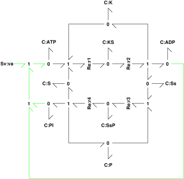
(a) System bond graph

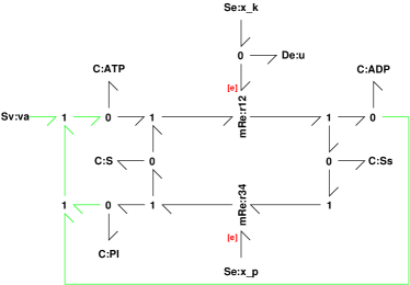
(b) Approximate system bond graph

Figure 6: A Biochemical Switch. (a) The bond graph of the biochemical switch of Beard and Qian [2] has four reactions Re:$\mathbf{r1}$ – Re:$\mathbf{r4}$ and nine substances. The external flow $v_{a}$ of ATP is required for the long-term operation of the switch which consumes ATP. (b) This switch can be approximated using the approximation of figure 5 whist retaining thermodynamic compliance.

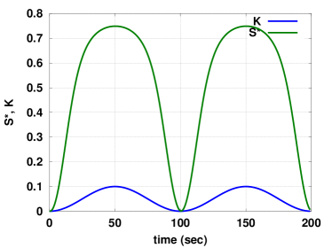
(a) $S^{\star}$ & $K$

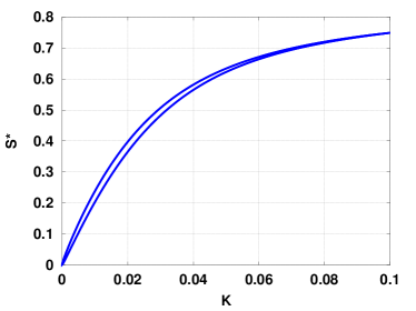
(b) $S^{\star}$ v. $K$

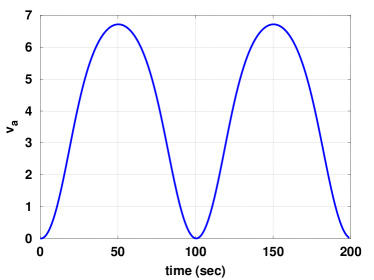
(c) $v_{a}$ – ATP flow

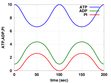
(d) ATP & $S$

Figure 7: A Biochemical Switch: simulation. (a) shows the time response of the amount of $S^{\star}$ to a sinusoidal variation in the amount of $K$. The biochemical switch both amplifies and distorts the signal. (b) plots $S^{\star}$ against $K$ to show the non-linear amplification effect. (c) shows the corresponding molar flow of ATP into the system and (d) the corresponding amounts of ATP, ADP and Pi.

Beard and Qian [2, §5.1.1] discuss a biochemical switch described by

$$S+ATP+K {\;\xrightleftharpoons{1}\;}KS KS {\;\xrightleftharpoons{2}\;}S^{\star}+ADP+K$$

$$S^{\star}+P {\;\xrightleftharpoons{3}\;}S^{\star}P S^{\star}P {\;\xrightleftharpoons{4}\;}S+Pi+P$$ (106)

These reactions represent a phosphorylation / dephosphorylation cycle. Protein $S$ is phosphorylated by kinase $K$, and is dephosphorylated by phosphatase $P$, where $S^{\star}$ represents the phosphorylated (active, perhaps) state of the protein. The corresponding bond graph appears in figure 6(a) where the external flow $v_{a}$ necessary to top up the ATP reservoir is included. This system contains 9 states and four reactions with mass-action kinetics. Using the approximation of §5.1, figure 5, this system can be approximated by the bond graph of 6(b). The approximate system has 5 states and two reactions with the reversible Michaelis-Menten kinetics of §5.1. It has the further advantage that the dynamics are explicitly modulated by the concentrations $x_{k}$ and $x_{p}$ of $K$ and $P$ respectively.

The bond graph of 6(b) clearly shows a biochemical cycle. It’s behaviour can be understood as follows. When $x_{k}$ is large. ATP drives $S$ though the reaction component Re:$\mathbf{r12}$ to create $S^{\star}$; and this flow is greater than that though Re:$\mathbf{r34}$ and so the amount of $S^{\star}$ increases at the expense of $S$. However, when $x_{k}$ is small the flow though Re:$\mathbf{r12}$ becomes less than that though Re:$\mathbf{r34}$ and amount of $S^{\star}$ decreases.

For the purposes of illustration, the following parameter values were used. With reference to Equation (104), $k_{m}=0$ and $\bar{\kappa}K_{c}=100$ for both reactions. With reference to Equations (3), $K_{ATP}=10$ and $K_{S}=K_{S*}=K_{ADP}=K_{PI}=1$. The initial states were: $x_{ATP}=10$, $x_{S}=x_{ADP}=1$ and $x_{S*}=x_{PI}=0$.

Figure 7 shows a simulation of the biochemical switch when ATP is replenished by setting

$$v_{a}=g_{a}\left(w_{atp}-x_{atp}\right)\text{ where }g_{a}=2\text{ and }w_{atp}=10$$ (107)

Equation (107) represents simple proportional feedback; in vivo, this would correspond to a cellular control system. Figure 7(a) shows the response of the amount of $S^{\star}$ to a sinusoidal variation in the amount of $K$. The biochemical switch both amplifies and distorts the signal. This effect is further shown in figure 7(b) where the amount of $S^{\star}$ is plotted against the amount of $K$. This is basically a high-gain saturating function. The hysteresis is due to the time constant of the feedback loop implied by Equation (107); the hysteresis reduces if either $g_{a}$ is increases or the frequency of the input sinusoid decreased. All biochemical cycles require free-energy transduction [1]. Figure 7(c) shows the molar flow of ATP into the system (and, as indicated in figure 6(b) the outflow of ADP and Pi) as a function of time; the ON state of the switch induces a flow of ATP using Equation (107) to replenish the ATP consumed by the cycle. Figure 7(d) shows the corresponding amounts of ATP, ADP and Pi. The controller does not exactly hold ATP at the desired level of $w_{atp}=10$; a higher gain controller would reduce the control error. As discussed by Beard and Qian [2, §5.1.1]: “$\dots$ a biochemical switch cannot function without a free energy input. No energy, no switch”. This can be simulated by setting $g_{a}=0$ in Equation (107) and forms Figure 1 of §A of the electronic supplementary material.

Approximate models of signalling network components have been advocated by Kraeutler et al. [68] and Ryall et al. [69] as an approach to understanding the behaviour of complex signalling networks. The models developed in this section could also be used for such a purpose, but with the advantage that the resulting model is thermodynamically compliant.

Model reduction of an enzymatic cycle model of the SERCA pump [70] is discussed in §C of the electronic supplementary material.

6 Hierarchical Modelling of Large Systems

One of the objectives of systems biology is to represent the network of biochemical reactions taking place in cells by computational models. Large-scale models of cellular metabolic and signalling networks have been constructed; for example, cardiac cell models which integrate electrophysiology, metabolism, signalling, and cellular mechanics have been developed in order to study cell physiology in normal and disease conditions [71].

In order to facilitate the development and reuse of such models, XML-based markup languages such as CellML [72] and SBML [73] have been created. These languages enable mathematical descriptions of biological processes to be stored in machine-readable formats, but put relatively little restriction on the formulation of the models themselves.

For example, CellML, which was originally developed in order to share models of cardiac cell dynamics, represents models as a number of component elements, each of which contains a number of variables (for example representing cell membrane potential, or an ionic concentration), the mathematical relationship between these variables (for example, the Nernst potential given as a function of the concentrations) expressed in MathML, and associated parameters. Such components can be connected to one another to form a model.

This construction allows a modular approach to modelling in which cellular processes and reactions can be broken down into components, which are then connected to form a model of the system under study [74]. However, there is no requirement that components adhere to the principles of conservation of mass, conservation of charge, or thermodynamic consistency. Nor is there currently any framework which would ensure thermodynamic consistency, or mass or charge conservation, for a model created by connecting components in this modular fashion, even if the components themselves were constructed as thermodynamic cycles.

The Bond Graph approach which we have outlined here provides such a framework for modular representation of components of biological systems, which can be assembled so as to preserve thermodynamic properties, charge and mass conservation, both in the individual components and in the overall system. Furthermore, the development of the Bond Graph Markup Language (BGML) by Borutzky [35] for the exchange and reuse of bond graph models, and associated software, provides the tools through which integration with representations such as CellML may be achieved.

The stoichiometric analysis of Section 3, and its relationship to causality, is illustrated by simple systems. However, the notion of bond graph causality, and the corresponding propagation of causality using the sequential causality assignment procedure [10, Chapter 5], is applicable to arbitarily large systems.

7 Conclusion

Based on the seminal work of Oster et al. [16], the fundamental concepts of network thermodynamics have been combined with more recent developments in the bond graph approach to system modelling to give a new approach to building dynamical models of biochemical networks within which compliance with thermodynamic principles is automatically satisfied. As noted in the Introduction, the bond graph is more than a sketch of a biochemical network; it can be directly interpreted by a computer and, moreover, has a number of features that enable key physical properties to be derived from the bond graph itself. It has been shown that stoichiometric properties, including the stoichiometric matrix $N$ and the left and right null-space matrices $G$ and $K$, can be directly derived from the bond graph using the concept of causality associated with bond graphs. The corresponding causal paths, when superimposed on the bond graph, directly indicate both pools (conserved moieties) and steady-state flux paths. The bond graph methodology includes a framework for approximating complex systems whilst retaining compliance with thermodynamic principles and this has been illustrated in two contexts: chains of reactions and the Michaelis-Menten approximation of enzyme-catalysed reactions.

As emphasised by Beard and Qian [2], living organisms are associated with non-equilibrium steady-states. For this reason, this paper has emphasised the role of external inputs to biochemical networks modelled by bond graphs. In particular, the example of §5.2, models a biochemical switch where the role of ATP as a power source is explicitly integrated into the bond graph model.

The bond graph approach is naturally modular in that networks of biochemical reactions can be connected by bonds whilst retaining compliance with thermodynamic principles. Modularity has been illustrated by simple examples and future work will develop appropriate software tools to build on this natural modularity.

Biochemical networks have non-linear dynamics which generate phenomena which cannot be generated by linear systems. Nevertheless, useful information can be obtained from linear models obtained by linearisation of non-linear systems. In the context of engineering systems theory, linearisation has been considered within the framework of sensitivity theory [75, 76]. In the context of biochemical networks, Metabolic Control Analysis (MCA) [77] is based on the sensitivity analysis of stoichiometric networks. The relationship of MCA to engineering concepts of sensitivity has been examined by Ingalls and Sauro [64], Ingalls [65] and Sauro [66]. Ingalls [65] has shown that standard engineering sensitivity theory can be applied to biochemical networks to derive frequency responses with respect to small perturbations in system parameters. Sensitivity and linearisation of systems described by bond graphs has been considered by an number of authors [78, 79, 80]. The bond graph approach has the advantage of retaining the system structure. Future work will look at bond graph based linearisation in the context of biochemical networks.

This paper has focused on deriving thermodynamically compliant biochemical reaction networks, and their thermodynamically compliant approximations, from elementary biochemical equations. It would be interesting to look at the inverse problem: Is a given ODE model of a system of biochemical reactions with non mass-action kinetics thermodynamically compliant and does it have a bond graph representation?

In addition to stoichiometric analysis, the bond graph approach can be used to directly investigate structural properties of dynamical systems such as controllability [62, 81] and invertiblity [82, 83, 59, 61]. Future work will look at bond graph based structural analysis in the context of biochemical networks.

The bond graph approach is based on the notion of power flow. For this reason, it has been much used for modelling multi-domain engineering systems with appropriate transducer models to interface domains. Thus for example: an electric motor or a piezo-electric actuator couples electrical and mechanical domains and a turbine or pump couples hydraulic and mechanical domains. We will build on the work of LeFèvre et al. [43] on chemo-mechanical transduction and the work of Karnopp [39] on chemo-electrical transduction to interface biochemical networks with systems involving muscle and excitable membranes.

We believe that, when combined with modern software tools, the bond graph approach provides a significant alternative hierarchical and modular modelling framework for complex biochemical systems in which compliance with thermodynamic principles is automatically satisfied.

Appendix A A biochemical switch : further simulations

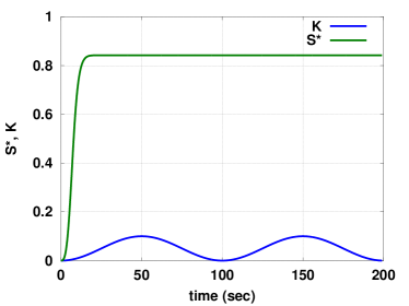
(a) $S^{\star}$ & $K$

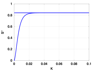
(b) $S^{\star}$ v. $K$

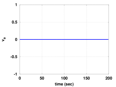
(c) $v_{a}$ – ATP flow

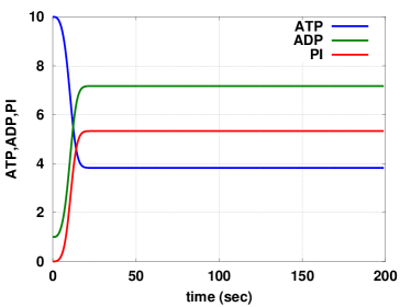
(d) ATP & $S$

Figure 8: A Biochemical Switch: simulation without ATP replenishment. The simulation is the same as that of Figure 7 of §5(b) of the paper except that ATP is not replenished and so the switch fails to function.

Appendix B Bimolecular reactions

Name	Bond Graph
(a) Bimolecular reaction
(b) Fast bimolecular reaction
(c) Simplified bimolecular reaction

Figure 9: Approximation of bimolecular reactions.

Thermodynamic cycles typically involve bimolecular reactions where, in bond graph terms, the chain of reactions discussed in Section 4 is augmented by branches. Figure 9(a) shows a reaction of the form $A+C{\;\xrightleftharpoons{}\;}B$ where the presence of $C$ gives the branched bond graph structure. The bonds at the left and right of Figure 9(a) form connections to the rest of a reaction network.

There are two approximations made to simplify this bimolecular reaction. As in Section 4 it is assumed that the reaction is fast and thus the Re component can be removed as in Figure 9(b). It is further assumed that the concentration of $C$ is approximately constant either due to replenishment or to a large pool; this is indicated in Figure 9(b) by replacing the component C:$\mathbf{C}$ by CS:$\mathbf{C}$: a capacitive source. As in Section 4, the removal of the Re component changes the causality of C:$\mathbf{B}$, but the causality of CS:$\mathbf{C}$ remains the same as that of C:$\mathbf{C}$.

Again, the equilibrium induced by the removal of the Re component leads to the state $x_{b}$ of C:$\mathbf{B}$ being determined by the states of the other two components:

$$x_{b} =\frac{K_{c}x_{c}K_{a}x_{a}}{K_{b}}$$

$$=\tilde{x}_{c}x_{a}$$ (108)

$$\text{where }\tilde{x}_{c} =\frac{K_{c}K_{a}}{K_{b}}x_{c}$$ (109)

$$\text{thus }x_{ab} =x_{a}+x_{b}=(1+\tilde{x}_{c})x_{a}$$ (110)

Unlike the unimolecular case, the chemical potentials $\mu_{1}$ and $\mu_{2}$ are different; in particular

$$\mu_{2}=\mu_{1}+RT\ln K_{c}x_{c}$$ (111)

Comparing Figures 9(b) and 9(c):

$$\mu_{1} =RT\ln K_{ab}x_{ab}=RT\ln K_{a}x_{a}$$ (112)

It follows from Equation (110) that:

$$K_{ab}=K_{a}\frac{x_{a}}{x_{ab}}=\frac{K_{a}}{1+\tilde{x}_{c}}$$ (113)

Using Equations (111), (112) and (113) it follows that:

$$\mu_{2} =RT\ln K_{ab}x_{ab}+RT\ln K_{c}x_{c}$$

$$=RT\ln K_{ab}x_{ab}K_{c}x_{c}$$

$$=RT\ln K_{ab}x_{ab}\frac{K_{b}}{K_{a}}\tilde{x}_{c}$$

$$=RT\ln K_{ba}x_{ab}$$ (114)

$$\text{where}K_{ba} =\frac{K_{b}\tilde{x}_{c}}{1+\tilde{x}_{c}}$$ (115)

Equations (113) and (114) correspond to the equations for $\alpha_{4}^{+}$ and $\alpha_{3}^{-}$ in the paper of Smith and Crampin [26, Equations (30) & (31)].

These simplification approaches for slow-fast reactions can naturally be applied to more complicated reaction schemes by application in a stepwise manner, each step of which preserves the underlying thermodynamic structure of the model. This can be automated, and can be used to generate different representations of an underlying model, as for example was done in our recent model of the cardiac sarcoplasmic/endoplasmic $\text{Ca}^{2+}$ (SERCA) pump. Such models consider enzyme mechanisms to be thermodynamic cycles. These are discussed below.

Appendix C Example: model reduction of an enzymatic cycle model of the SERCA pump

(a) 9-state (8-state cycle) model

(b) 3-state reduced enzymatic cycle model

Figure 10: Schematic of SERCA pump model. (a) for the cardiac SERCA pump (where calcium binding mechanism is assumed to be fully cooperative); and (b) reduced 3-state model, modified from Tran et al. [70]. The dotted boxes in (a) show partial sub-systems of the model which are simplified to reduce the 9-state to the 3-state model.

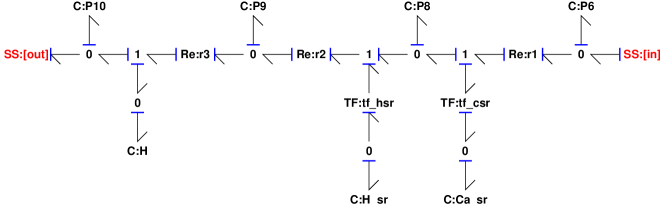
(a) Bond graph of partial system

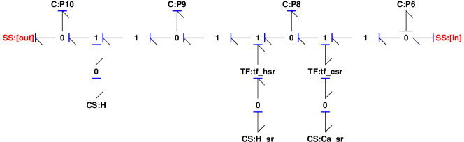
(b) Bond of simplified partial system

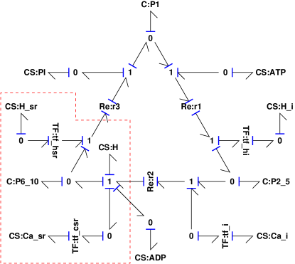
(c) Bond graph of simplified pump

Figure 11: Bond Graph of Partial SERCA pump model. (a) Shows the bond graph corresponding to the subsystem with states $P_{6}$–$P_{10}$ of Figure 10(a) and the seven C components in integral causality correspond to the seven states. (b) The simplified subsystem has one C component in integral causality and thus only one state. (c) This subsystem is shown within the dashed box as part of the overall simplified model. C:$\mathbf{P6\_10}$ represents the composite state of the subsystem and the CS components the corresponding constant concentrations.

Tran et al. [70] present a thermodynamic enzyme cycle model of the cardiac sarcoplasmic/endoplasmic $\text{Ca}^{2+}$ ATPase (SERCA) pump. A multi-state model is constructed which incorporates binding of different molecular species to the SERCA protein, including transported calcium ions, co-transported and competitively binding hydrogen ions, ATP and its hydrolysis products ADP, Pi and hydrogen ion, and which represents conformational changes of the protein in the enzymatic cycle, and associated free energy transduction. This generates a thermodynamically constrained enzyme cycle model for SERCA, however the model has a large number of reaction steps and associated parameters, and, using methods akin to those in Section 4, the model is reduced from the nine-state, nine-reaction model of Figure 10(a) to the three-state, three-reaction model of Figure 10(b) by simplifying the reaction mechanism corresponding to states $P_{2}$–$P_{5}$ and to states $P_{6}$–$P_{10}$ by assuming rapid equilibrium for calcium and hydrogen ion association-dissociation reactions.

To illustrate the bond graph equivalent of this procedure, Figure 11(a) gives the reaction mechanism corresponding to states $P_{6}$–$P_{10}$. Using the approach of Section B, this is reduced to the bond graph of Figure 11(b). The bond graph corresponding to Figure 10(b) is given in Figure 11(c) where the dotted line delineates the approximation to reaction mechanism corresponding to states $P_{6}$–$P_{10}$.

The three reaction components Re:$\mathbf{r1}$–Re:$\mathbf{r3}$ correspond to flows:

$$v_{1} =\alpha_{1}^{+}x_{1}-\alpha_{1}^{-}x_{2}$$ (116)

$$v_{2} =\alpha_{2}^{+}x_{2}-\alpha_{2}^{-}x_{3}$$ (117)

$$v_{3} =\alpha_{3}^{+}x_{3}-\alpha_{3}^{-}x_{1}$$ (118)

where $x_{1}$, $x_{2}$ and $x_{3}$ are the state occupancy probabilities of states C:$\mathbf{P_{1}}$, C:$\mathbf{P_{2-5}}$ and C:$\mathbf{P_{6-10}}$. Using methods akin to those of Section B, Tran et al. [70] show that:

$$\alpha^{+}_{1} = k^{+}_{1}\mathrm{[MgATP]},$$ (119)

$$\alpha^{+}_{2} = \dfrac{k^{+}_{2}\mathrm{\widetilde{Ca}^{2}_{i}}}{\mathrm{\widetilde{Ca}^{2}_{i}}(1+\mathrm{\widetilde{\,H}_{i}^{n}})+\mathrm{\widetilde{\,H}_{i}^{n}}(1+\mathrm{\widetilde{H}_{1}})},$$ (120)

$$\alpha^{+}_{3} = \dfrac{k^{+}_{3}\mathrm{\widetilde{\,H}_{sr}^{n}}}{\mathrm{\widetilde{H}}(1+\mathrm{\widetilde{Ca}^{2}_{sr}})+\mathrm{\widetilde{\,H}_{sr}^{n}}(1+\mathrm{\widetilde{H}})}$$ (121)

and the apparent backward rate constants are:

$$\alpha^{-}_{1} = \dfrac{k^{-}_{1}\mathrm{\widetilde{\,H}_{i}^{n}}}{\mathrm{\widetilde{Ca}^{2}_{i}}(1+\mathrm{\widetilde{\,H}_{i}^{n}})+\mathrm{\widetilde{\,H}_{i}^{n}}(1+\mathrm{\widetilde{H}_{1}})},$$ (122)

$$\alpha^{-}_{2} = \dfrac{k^{-}_{2}\mathrm{[MgADP]}\mathrm{\widetilde{Ca}^{2}_{sr}}\mathrm{\widetilde{\,H}_{sr}^{n}}}{\mathrm{\widetilde{H}}(1+\mathrm{\widetilde{Ca}^{2}_{sr}})+\mathrm{\widetilde{\,H}^{n}_{sr}}(1+\mathrm{\widetilde{H}})},$$ (123)

$$\alpha^{-}_{3} = k^{-}_{3}\mathrm{[Pi]}$$ (124)

where

$$\mathrm{\widetilde{Ca}_{i}}=\dfrac{\mathrm{[Ca^{2+}]_{i}}}{K_{d,Cai}}, \mathrm{\widetilde{H}_{i}}=\dfrac{\mathrm{[H^{+}]}}{K_{d,Hi}}, \mathrm{\widetilde{H}_{1}}=\dfrac{\mathrm{[H^{+}]}}{K_{d,H1}},$$

$$\mathrm{\widetilde{Ca}_{sr}}=\dfrac{\mathrm{[Ca^{2+}]_{sr}}}{K_{d,Casr}}, \mathrm{\widetilde{H}_{sr}}=\dfrac{\mathrm{[H^{+}]}}{K_{d,Hsr}}, \mathrm{\widetilde{H}}=\dfrac{\mathrm{[H^{+}]}}{K_{d,H}}$$

As discussed further below, the purpose of this model reduction is not to reduce dynamical complexity but rather to reduce the number of unknown parameters to a value consistent with available experimental data. As demonstrated here, and discussed by Tran et al. [70], this approach retains the thermodynamic properties of the full enzyme cycle model while reducing the number of unknown parameters.

The major advantage of this approach is that in constructing models such as this we usually do not know, a priori, the full set of parameters associated with the enzymatic cycle. A subset of the parameters, such as the free energy of hydrolysis of ATP, are known; and these values carry through to the reduced model. However, the majority of parameters (binding and unbinding rates, which are reduced to dissociation constants in the rapid equilibrium approximation) are typically not known and must be estimated by fitting the resulting model to data (namely the steady state cycling rate of the model, as a function of concentrations of the different species, fitted to the data where rate of calcium transport is measured for different concentrations of calcium, pH and metabolites). This parameter estimation process is made significantly more tractable following reduction of the model to the simpler cycle, without compromising the thermodynamic properties and the prior knowledge incorporated in the full multi-state construction.

References

- Hill [1989] Terrell L Hill. Free energy transduction and biochemical cycle kinetics. Springer-Verlag, New York, 1989.
- Beard and Qian [2010] Daniel A Beard and Hong Qian. Chemical biophysics: quantitative analysis of cellular systems. Cambridge University Press, 2010.
- Keener and Sneyd [2009] James P Keener and James Sneyd. Mathematical Physiology: I: Cellular Physiology, volume 1. Springer, 2nd edition, 2009.
- Katchalsky and Curran [1965] A. Katchalsky and Peter F. Curran. Nonequilibrium Thermodynamics in Biophysics. Harvard University Press, Cambridge, Massachusetts., 1965.
- Cellier [1991] F. E. Cellier. Continuous system modelling. Springer-Verlag, 1991.
- Gunawardena [2014] Jeremy Gunawardena. Time-scale separation – Michaelis and Menten’s old idea, still bearing fruit. FEBS Journal, 281(2):473–488, 2014. ISSN 1742-4658. doi:10.1111/febs.12532.
- Paynter [1992] H.M. Paynter. An epistemic prehistory of bond graphs. In P.C. Breedveld and G. Dauphin-Tanguy, editors, Bond Graphs for Engineers, pages 3–17. North-Holland, Amsterdam, 1992.
- Gawthrop and Smith [1996] P. J. Gawthrop and L. P. S. Smith. Metamodelling: Bond Graphs and Dynamic Systems. Prentice Hall, Hemel Hempstead, Herts, England., 1996. ISBN 0-13-489824-9.
- Borutzky [2011] Wolfgang Borutzky. Bond Graph Modelling of Engineering Systems: Theory, Applications and Software Support. Springer, 2011. ISBN 9781441993670.
- Karnopp et al. [2012] Dean C Karnopp, Donald L Margolis, and Ronald C Rosenberg. System Dynamics: Modeling, Simulation, and Control of Mechatronic Systems. John Wiley & Sons, 5th edition, 2012. ISBN 978-0470889084.
- Gawthrop and Bevan [2007] Peter J Gawthrop and Geraint P Bevan. Bond-graph modeling: A tutorial introduction for control engineers. IEEE Control Systems Magazine, 27(2):24–45, April 2007. doi:10.1109/MCS.2007.338279.
- Palsson [2006] Bernhard Palsson. Systems biology: properties of reconstructed networks. Cambridge University Press, 2006. ISBN 0521859034.
- Palsson [2011] Bernhard Palsson. Systems Biology: Simulation of Dynamic Network States. Cambridge University Press, 2011.
- Alon [2007] Uri Alon. Introduction to Systems Biology: Design Principles of Biological Networks. CRC press, 2007.
- Klipp et al. [2011] Edda Klipp, Wolfram Liebermeister, Christoph Wierling, Axel Kowald, Hans Lehrach, and Ralf Herwig. Systems biology. Wiley-Blackwell, 2011.
- Oster et al. [1971] George Oster, Alan Perelson, and Aharon Katchalsky. Network thermodynamics. Nature, 234:393–399, December 1971. doi:10.1038/234393a0.
- Oster et al. [1973] George F. Oster, Alan S. Perelson, and Aharon Katchalsky. Network thermodynamics: dynamic modelling of biophysical systems. Quarterly Reviews of Biophysics, 6(01):1–134, 1973. doi:10.1017/S0033583500000081.
- Oster and Perelson [1974] G. Oster and A. Perelson. Chemical reaction networks. Circuits and Systems, IEEE Transactions on, 21(6):709 – 721, November 1974. ISSN 0098-4094. doi:10.1109/TCS.1974.1083946.
- Oster and Auslander [1971a] George F. Oster and David M. Auslander. Topological representations of thermodynamic systems–I. basic concepts. Journal of the Franklin Institute, 292(1):1 – 17, 1971a. ISSN 0016-0032. doi:10.1016/0016-0032(71)90037-8.
- Oster and Auslander [1971b] George F. Oster and David M. Auslander. Topological representations of thermodynamic systems–II. some elemental subunits for irreversible thermodynamics. Journal of the Franklin Institute, 292(2):77 – 92, 1971b. ISSN 0016-0032. doi:10.1016/0016-0032(71)90196-7.
- Kohl et al. [2010] P Kohl, Edmund J Crampin, T A Quinn, and D Noble. Systems Biology: An Approach. Clinical Pharmacology & Therapeutics, 88(1):25–33, June 2010.
- Aldridge et al. [2006] Bree B. Aldridge, John M. Burke, Douglas A. Lauffenburger, and Peter K. Sorger. Physicochemical modelling of cell signalling pathways. Nat Cell Biol, 8:1195–1203, November 2006. ISSN 1465-7392. doi:10.1038/ncb1497.
- Smith et al. [2007] Nicolas P Smith, Edmund J Crampin, Steven A Niederer, James B Bassingthwaighte, and Daniel A Beard. Computational biology of cardiac myocytes: proposed standards for the physiome. The Journal of experimental biology, 210(Pt 9):1576–1583, May 2007.
- Hunter et al. [2008] Peter J Hunter, Edmund J Crampin, and Poul M F Nielsen. Bioinformatics, multiscale modeling and the IUPS Physiome Project. Briefings in Bioinformatics, 9(4):333–343, July 2008.
- Hunter et al. [2012] Peter Hunter, Chris Bradley, Randall Britten, David Brooks, Luigi Carotenuto, Richard Christie, Alejandro Frangi, Alan Garny, David Ladd, David Nickerson Caton Little, Poul Nielsen, Andrew Miller, Xavier Planes, Martin Steghoffer, Alistair Young, and Tommy Yu. The VPH-Physiome Project: standards, tools and databases for multi-scale physiological modelling. In Ambrosi D, Quarteroni A, and Rozza G, editors, Modeling of Physiological Flows., pages 1–23. Springer-Verlag Italia, November 2012.
- Smith and Crampin [2004] N.P. Smith and E.J. Crampin. Development of models of active ion transport for whole-cell modelling: cardiac sodium-potassium pump as a case study. Progress in Biophysics and Molecular Biology, 85(2-3):387 – 405, 2004. doi:10.1016/j.pbiomolbio.2004.01.010.
- Tran et al. [2009a] Kenneth Tran, Nicolas P Smith, Denis S Loiselle, and Edmund J Crampin. A Thermodynamic Model of the Cardiac Sarcoplasmic/Endoplasmic Ca2+ (SERCA) Pump. Biophysical Journal, 96(5):2029–2042, 2009a.
- Beard [2005] Daniel A Beard. A biophysical model of the mitochondrial respiratory system and oxidative phosphorylation. PLoS Computational Biology, 1(4):e36, 2005.
- Beard et al. [2004] Daniel A Beard, Eric Babson, Edward Curtis, and Hong Qian. Thermodynamic constraints for biochemical networks. Journal of Theoretical Biology, 228(3):327–333, June 2004.
- Beard et al. [2002] Daniel A. Beard, Shoudan Liang, and Hong Qian. Energy balance for analysis of complex metabolic networks. Biophysical Journal, 83(1):79 – 86, 2002. ISSN 0006-3495. doi:10.1016/S0006-3495(02)75150-3.
- Feist et al. [2007] Adam M Feist, Christopher S Henry, Jennifer L Reed, Markus Krummenacker, Andrew R Joyce, Peter D Karp, Linda J Broadbelt, Vassily Hatzimanikatis, and Bernhard O Palsson. A genome-scale metabolic reconstruction for Escherichia coli K-12 MG1655 that accounts for 1260 ORFs and thermodynamic information. Molecular Systems Biology, 3, June 2007.
- Soh and Hatzimanikatis [2010] Keng Cher Soh and Vassily Hatzimanikatis. Network thermodynamics in the post-genomic era. Current Opinion in Microbiology, 13(3):350–357, June 2010.
- Ballance et al. [2005] Donald J. Ballance, Geraint P. Bevan, Peter J. Gawthrop, and Dominic J. Diston. Model transformation tools (MTT): The open source bond graph project. In Proceedings of the 2005 International Conference On Bond Graph Modeling and Simulation (ICBGM’05), Simulation Series, pages 123–128, New Orleans, U.S.A., January 2005. Society for Computer Simulation.
- Cellier and Nebot [2005] F.E. Cellier and A. Nebot. The modelica bond graph library. In Proceedings 4th International Modelica Conference, volume 1, pages 57–65, Hamburg, Germany, 2005.
- Borutzky [2006] W. Borutzky. BGML – a novel XML format for the exchange and the reuse of bond graph models of engineering systems. Simulation Modelling Practice and Theory, 14(7):787 – 808, 2006. ISSN 1569-190X. doi:10.1016/j.simpat.2006.01.002.
- Cellier and Greifeneder [2008] F.E. Cellier and J. Greifeneder. Thermobondlib - a new modelica library for modeling convective flows. In Proceedings of the 6th International Modelica Conference, pages 163 – 172, Bielefeld, Deutschland, March 2008.
- Cellier and Greifeneder [2009] F.E. Cellier and J. Greifeneder. Modeling chemical reactions in modelica by use of chemo-bonds. In Proceedings 7th Modelica Conference, Como, Italy, September 2009.
- de la Calle et al. [2013] Alberto de la Calle, Francois E. Cellier, Luis J. Yebra, and Sebastian Dormido. Improvements in bondlib the modelica bond graph library. In Proceeding of the 8th EUROSIM Congress, Cardiff, Cardiff, Wales, September 2013.
- Karnopp [1990] Dean Karnopp. Bond graph models for electrochemical energy storage : electrical, chemical and thermal effects. Journal of the Franklin Institute, 327(6):983 – 992, 1990. ISSN 0016-0032. doi:10.1016/0016-0032(90)90073-R.
- Thoma and Atlan [1977] Jean U. Thoma and Henri Atlan. Network thermodynamics with entropy stripping. Journal of the Franklin Institute, 303(4):319 – 328, 1977. ISSN 0016-0032. doi:10.1016/0016-0032(77)90114-4.
- Greifeneder and Cellier [2012] J. Greifeneder and F.E. Cellier. Modeling chemical reactions using bond graphs. In Proceedings ICBGM12, 10th SCS Intl. Conf. on Bond Graph Modeling and Simulation, pages 110–121, Genoa, Italy, 2012.
- Thoma and Atlan [1985] Jean Thoma and Henri Atlan. Osmosis and hydraulics by network thermodynamics and bond graphs. Journal of the Franklin Institute, 319(1-2):217 – 226, 1985. ISSN 0016-0032. doi:10.1016/0016-0032(85)90075-4.
- LeFèvre et al. [1999] Jacques LeFèvre, Laurent LeFèvre, and Bernadette Couteiro. A bond graph model of chemo-mechanical transduction in the mammalian left ventricle. Simulation Practice and Theory, 7(5-6):531–552, 1999. ISSN 0928-4869. doi:10.1016/S0928-4869(99)00023-3.
- Fuchs [1996] Hans U. Fuchs. The Dynamics of Heat. Springer, New York, 1996.
- Job and Herrmann [2006] G Job and F Herrmann. Chemical potential – a quantity in search of recognition. European Journal of Physics, 27(2):353–371, 2006. doi:10.1088/0143-0807/27/2/018.
- Cellier [1992] F. E. Cellier. Hierarchical non-linear bond graphs: a unified methodology for modeling complex physical systems. SIMULATION, 58(4):230–248, 1992. doi:10.1177/003754979205800404.
- Gawthrop and Smith [1992] P. J. Gawthrop and L. Smith. Causal augmentation of bond graphs with algebraic loops. Journal of the Franklin Institute, 329(2):291–303, 1992. doi:10.1016/0016-0032(92)90035-F.
- Sueur and Dauphin-Tanguy [1991] C. Sueur and G. Dauphin-Tanguy. Bond graph approach to multi-time scale systems analysis. Journal of the Franklin Institute, 328(5 6):1005 – 1026, 1991. ISSN 0016-0032. doi:10.1016/0016-0032(91)90066-C.
- Qian and Beard [2005] Hong Qian and Daniel A. Beard. Thermodynamics of stoichiometric biochemical networks in living systems far from equilibrium. Biophysical Chemistry, 114(2-3):213 – 220, 2005. ISSN 0301-4622. doi:10.1016/j.bpc.2004.12.001.
- Qian et al. [2003] Hong Qian, Daniel A. Beard, and Shou-dan Liang. Stoichiometric network theory for nonequilibrium biochemical systems. European Journal of Biochemistry, 270(3):415–421, 2003. ISSN 1432-1033. doi:10.1046/j.1432-1033.2003.03357.x.
- Van Rysselberghe [1958] Pierre Van Rysselberghe. Reaction rates and affinities. The Journal of Chemical Physics, 29(3):640–642, 1958. doi:10.1063/1.1744552.
- Boudart [1983] M. Boudart. Thermodynamic and kinetic coupling of chain and catalytic reactions. The Journal of Physical Chemistry, 87(15):2786–2789, 1983. doi:10.1021/j100238a018.
- Laidler [1985] Keith J. Laidler. René Marcelin (1885-1914), a short-lived genius of chemical kinetics. Journal of Chemical Education, 62(11):1012, 1985. doi:10.1021/ed062p1012.
- Jamshidi and Palsson [2011] Neema Jamshidi and Bernhard Palsson. Metabolic network dynamics: Properties and principles. In Jennifer Southgate Werner Dubitzky and Hendrik Fuss, editors, Understanding the Dynamics of Biological Systems, pages 19–37. Springer, Berlin, 2011. doi:10.1007/978-1-4419-7964-3_2.
- Schilling et al. [2000] Christophe H. Schilling, David Letscher, and Bernhard Palsson. Theory for the systemic definition of metabolic pathways and their use in interpreting metabolic function from a pathway-oriented perspective. Journal of Theoretical Biology, 203(3):229 – 248, 2000. ISSN 0022-5193. doi:10.1006/jtbi.2000.1073.
- Schuster et al. [2002] S. Schuster, C. Hilgetag, J.H. Woods, and D.A. Fell. Reaction routes in biochemical reaction systems: Algebraic properties, validated calculation procedure and example from nucleotide metabolism. Journal of Mathematical Biology, 45(2):153–181, 2002. ISSN 0303-6812. doi:10.1007/s002850200143.
- Famili and Palsson [2003a] Iman Famili and Bernhard O. Palsson. Systemic metabolic reactions are obtained by singular value decomposition of genome-scale stoichiometric matrices. Journal of Theoretical Biology, 224(1):87 – 96, 2003a. ISSN 0022-5193. doi:10.1016/S0022-5193(03)00146-2.
- Famili and Palsson [2003b] Iman Famili and Bernhard O. Palsson. The convex basis of the left null space of the stoichiometric matrix leads to the definition of metabolically meaningful pools. Biophysical Journal, 85(1):16 – 26, 2003b. ISSN 0006-3495. doi:10.1016/S0006-3495(03)74450-6.
- Gawthrop [2000a] Peter J Gawthrop. Physical interpretation of inverse dynamics using bicausal bond graphs. Journal of the Franklin Institute, 337(6):743–769, 2000a. doi:10.1016/S0016-0032(00)00051-X.
- Ngwompo et al. [2001] R. Ngwompo, S. Scavarda, and D. Thomasset. Physical model-based inversion in control systems design using bond graph representation part 2: applications. Proceedings of the I MECH E Part I Journal of Systems and Control Engineering, 215(2):105–112, April 2001.
- Marquis-Favre and Jardin [2011] Wilfrid Marquis-Favre and Audrey Jardin. Bond graphs and inverse modeling for mechatronic system design. In Wolfgang Borutzky, editor, Bond Graph Modelling of Engineering Systems, pages 195–226. Springer New York, 2011. ISBN 978-1-4419-9368-7. doi:10.1007/978-1-4419-9368-7-6.
- Sueur and Dauphin-Tanguy [1989] C. Sueur and G. Dauphin-Tanguy. Structural controllability/observability of linear systems represented by bond graphs. Journal of the Franklin Institute, 326:869–883, 1989.
- Reder [1988] Christine Reder. Metabolic control theory: A structural approach. Journal of Theoretical Biology, 135(2):175 – 201, 1988. ISSN 0022-5193. doi:10.1016/S0022-5193(88)80073-0.
- Ingalls and Sauro [2003] Brian P. Ingalls and Herbert M. Sauro. Sensitivity analysis of stoichiometric networks: an extension of metabolic control analysis to non-steady state trajectories. Journal of Theoretical Biology, 222(1):23 – 36, 2003. ISSN 0022-5193. doi:10.1016/S0022-5193(03)00011-0.
- Ingalls [2004] Brian P. Ingalls. A frequency domain approach to sensitivity analysis of biochemical networks. The Journal of Physical Chemistry B, 108(3):1143–1152, 2004. doi:10.1021/jp036567u.
- Sauro [2009] H.M. Sauro. Network dynamics. In Reneé Ireton, Kristina Montgomery, Roger Bumgarner, Ram Samudrala, and Jason McDermott, editors, Computational Systems Biology, volume 541 of Methods in Molecular Biology, pages 269–309. Humana Press, 2009. ISBN 978-1-58829-905-5. doi:10.1007/978-1-59745-243-4_13.
- Ingalls [2013] Brian P. Ingalls. Mathematical Modelling in Systems Biology. MIT Press, 2013.
- Kraeutler et al. [2010] Matthew Kraeutler, Anthony Soltis, and Jeffrey Saucerman. Modeling cardiac beta-adrenergic signaling with normalized-hill differential equations: comparison with a biochemical model. BMC Systems Biology, 4(1):157, 2010. ISSN 1752-0509. doi:10.1186/1752-0509-4-157.
- Ryall et al. [2012] Karen A. Ryall, David O. Holland, Kyle A. Delaney, Matthew J. Kraeutler, Audrey J. Parker, and Jeffrey J. Saucerman. Network reconstruction and systems analysis of cardiac myocyte hypertrophy signaling. Journal of Biological Chemistry, 287(50):42259–42268, 2012. doi:10.1074/jbc.M112.382937.
- Tran et al. [2009b] Kenneth Tran, Nicolas P. Smith, Denis S. Loiselle, and Edmund J. Crampin. A thermodynamic model of the cardiac sarcoplasmic/endoplasmic Ca2+ (SERCA) pump. Biophysical Journal, 96(5):2029 – 2042, 2009b. ISSN 0006-3495. doi:10.1016/j.bpj.2008.11.045.
- Fink et al. [2011] Martin Fink, Steven A. Niederer, Elizabeth M. Cherry, Flavio H. Fenton, Jussi T. Koivumaki, Gunnar Seemann, Rudiger Thul, Henggui Zhang, Frank B. Sachse, Dan Beard, Edmund J. Crampin, and Nicolas P. Smith. Cardiac cell modelling: Observations from the heart of the cardiac physiome project. Progress in Biophysics and Molecular Biology, 104(1-3):2 – 21, 2011. ISSN 0079-6107. doi:10.1016/j.pbiomolbio.2010.03.002.
- Lloyd et al. [2004] Catherine M Lloyd, Matt DB Halstead, and Poul F Nielsen. CellML: its future, present and past. Progress in Biophysics and Molecular Biology, 85(2):433–450, 2004.
- Hucka et al. [2003] M Hucka, A Finney, H M Sauro, H Bolouri, J C Doyle, H Kitano, A P Arkin, B J Bornstein, D Bray, A Cornish-Bowden, A A Cuellar, S Dronov, E D Gilles, M Ginkel, V Gor, I I Goryanin, W J Hedley, T C Hodgman, J H Hofmeyr, P J Hunter, N S Juty, J L Kasberger, A Kremling, U Kummer, N Le Novère, L M Loew, D Lucio, P Mendes, E Minch, E D Mjolsness, Y Nakayama, M R Nelson, P F Nielsen, T Sakurada, J C Schaff, B E Shapiro, T S Shimizu, H D Spence, J Stelling, K Takahashi, M Tomita, J Wagner, and J Wang. The systems biology markup language (SBML): a medium for representation and exchange of biochemical network models. Bioinformatics, 19(4):524–531, March 2003.
- Cooling et al. [2008] M.T. Cooling, P. Hunter, and E.J. Crampin. Modelling biological modularity with CellML. Systems Biology, IET, 2(2):73 –79, March 2008. ISSN 1751-8849. doi:10.1049/iet-syb:20070020.
- Frank [1978] Paul M. Frank. Introduction to System Sensitivity Theory. Academic Press, New York, 1978.
- Rosenwasser and Yusupov [2000] Efim Rosenwasser and Rafael Yusupov. Sensitivity of Automatic Control Systems. CRC press, Boca Raton, 2000.
- Heinrich and Schuster [1996] Reinhart Heinrich and Stefan Schuster. The regulation of cellular systems. Chapman & Hall New York, 1996.
- Karnopp [1977] Dean Karnopp. Power and energy in linearized physical systems. Journal of the Franklin Institute, 303(1):85 – 98, 1977. ISSN 0016-0032. doi:10.1016/0016-0032(77)90078-3.
- Gawthrop [2000b] Peter J Gawthrop. Sensitivity bond graphs. Journal of the Franklin Institute, 337(7):907–922, November 2000b. doi:10.1016/S0016-0032(00)00052-1.
- Gawthrop and Ronco [2000] Peter J. Gawthrop and Eric Ronco. Estimation and control of mechatronic systems using sensitivity bond graphs. Control Engineering Practice, 8(11):1237–1248, November 2000. doi:10.1016/S0967-0661(00)00062-9.
- Sueur and Dauphin-Tanguy [1997] C. Sueur and G. Dauphin-Tanguy. Controllability indices for structured systems. Linear Algebra and its Applications, 250:275–287, 1997.
- Ngwompo et al. [1996] R. Fotsu Ngwompo, S. Scavarda, and D. Thomasset. Inversion of linear time-invariant siso systems modelled by bond graph. Journal of the Franklin Institute, 333:157–174, March 1996.
- Ngwompo and Gawthrop [1999] Roger F Ngwompo and Peter J Gawthrop. Bond graph based simulation of nonlinear inverse systems using physical performance specifications. Journal of the Franklin Institute, 336(8):1225–1247, November 1999. doi:10.1016/S0016-0032(99)00032-0.