UMBILICITY AND CHARACTERIZATION OF PANSU SPHERES IN THE HEISENBERG GROUP

Abstract.

For $n\geq 2$ we define a notion of umbilicity for hypersurfaces in the Heisenberg group $H_{n}$. We classify umbilic hypersurfaces in some cases, and prove that Pansu spheres are the only umbilic spheres with positive constant $p($or horizontal)-mean curvature in $H_{n}$ up to Heisenberg translations.

1. Introduction and statement of the results

In classical differential geometry, we have the notion of umbilicity for a point in a hypersurface of the Euclidean space $R^{n}$. A connected, closed umbilic hypersurface of $R^{n}$ (i.e., all the points are umbilic) is shown to be a sphere. On the other hand, we have the Alexandrov theorem which says that a closed (compact with no boundary) hypersurface of positive constant mean curvature in $R^{n}$ must be a sphere. The original proof of Alexandrov’s theorem ([1]) is based on a reflection principle. Reflect the hypersurface $S$ across a hyperplane $P.$ Move $P$ until the reflected hypersurface touches the original hypersurface $S.$ The reflected hypersurface must coincide with $S$ by the strong maximum principle. Analytic proofs of Alexandrov’s theorem were given much later. In 1991 Montiel and Ros ([13]) gave a relatively elementary proof through the characterization of spheres by the umbilicity.

For a hypersurface in the Heisenberg group $H_{n}$ (see Section 2 for some basic material), we can still talk about mean curvature, called $p($or horizontal)-mean curvature $H$ (see Section 2 for the definition). A hypersurface defined by such $H$ $=$ $0$ is called $p$(horizontal)-minimal. Such $p$-minimal hypersurfaces or hypersurfaces with prescribed $p$-mean curvature have been extensively studied in the last ten years (see, for instance, [14], [2], [5], [15], [7], [16], [18], [8], [3], [6], [17], [4], and references therein).

By analogy with the Euclidean situation, we can ask if an Alexandrov-type theorem holds for the Heisenberg situation. The reflection principle doesn’t seem to work generally in this situation. In the case $n$ $=$ $1,$ Ritore and Rosales ([18]) showed that an Alexandrov-type theorem still holds. Their proof relies on the analysis of characteristic curves and singular set developed in [5]. For $n$ $\geq$ $2,$ on the other hand, we may invoke the method of Montiel and Ros to study the Alexandrov-type problem. So the first thing is to characterize, in this case, Pansu spheres (having positive constant $p$-mean curvature; see (1.6)) in terms of some notion of umbilicity. In this paper, we give a definition of umbilicity. We classify umbilic hypersurfaces in some cases, and carry out a characterization of Pansu spheres in $H_{n}$.

Let $\Sigma$ be a $C^{2}$ smooth (further assume the regular part is $C^{\infty}$ smooth; see below) hypersurface of the Heisenberg group $H_{n}$. Throughout this paper, we always assume $\Sigma$ is immersed and $n$ $\geq$ $2$. Let $\xi$ ($J$, resp.) denote the standard contact ($CR$, resp.) structure on $H_{n},$ defined by the kernel of the contact form

$$\Theta=dt+\sum_{j=1}^{n}(x_{j}dy_{j}-y_{j}dx_{j})$$

(see [9], [11], or Section 2). A point $p$ $\in$ $\Sigma$ is called singular if $\xi$ $=$ $T\Sigma$ at $p$. Otherwise $p$ is called regular or nonsingular (i.e., $\xi$ is transversal to $T\Sigma)$. Let $S_{\Sigma}$ denote the set of singular points, which is a closed subset of $\Sigma.$ We will further assume the regular part $\Sigma\backslash S_{\Sigma}$ is $C^{\infty}$ smooth. For a regular point, we define $\xi^{\prime}$ $\subset$ $\xi$ $\cap$ $T\Sigma$ by

(1.1) $$\xi^{\prime}=(\xi\cap T\Sigma)\cap J(\xi\cap T\Sigma).$$

Let ($\xi^{\prime}$)^⊥ denote the space of vectors in $\xi$, perpendicular to $\xi^{\prime}$ with respect to the Levi metric $G$ :$=$ $\frac{1}{2}d\Theta(\cdot,J\cdot)$ $=$ $\sum_{j=1}^{n}[(dx_{j})^{2}+(dy_{j})^{2}].$ It is not hard to see $\dim(\xi$ $\cap$ $T\Sigma)$ $\cap$ ($\xi^{\prime}$)^⊥ $=$ $1.$ Take $e_{n}$ $\in$ ($\xi$ $\cap$ $T\Sigma)$ $\cap$ ($\xi^{\prime}$)^⊥ of unit length. Define the horizontal normal $e_{2n}$ :$=$ $Je_{n}$. Let $\nabla$ denote the pseudohermitian connection associated to $(J,\Theta)$ (see Section 2 for an explanation). Observe that $\nabla_{e_{n}}e_{2n}$ $\in$ $\xi$ is perpendicular to $e_{2n}.$ So we can write $-\nabla_{e_{n}}e_{2n}$ $=$ $le_{n}$ modulo $\xi^{\prime}$ for some function $l.$ Now define the vector field $X_{n}$ $\in$ $\xi^{\prime}$ by

(1.2) $$X_{n}:=\nabla_{e_{n}}e_{2n}+le_{n}.$$

This vector field is uniquely defined on the regular part of $\Sigma$. Note that if $p\in\Sigma$ is a regular point such that $X_{n}(p)=0$, then we have

(1.3) $$\left(-\nabla e_{2n}+\alpha J^{\prime}\right)(\xi^{\prime})\subset\xi^{\prime},$$

(see Proposition 2.3) where

(1.4) $$J^{\prime}:=J\text{ on }\xi^{\prime}\text{ and }J^{\prime}e_{n}:=0$$

(cf. (2.7)). Hence we can regard this operator $-\nabla e_{2n}+\alpha J^{\prime}$ originally defined on $\xi\cap T\Sigma$ (see (2.8)) as an endomorphism on $\xi^{\prime}$. This symmetric second fundamental form or shape operator first appeared in Ritoré’s paper (see page 52 in [17]). Conversely, if $\xi^{\prime}$ is invariant under the operator $-\nabla e_{2n}+\alpha J^{\prime}$, then $X_{n}=0$ (see also Proposition 2.3). In addition, it is self-adjoint (see Proposition 2.2). So we immediately have the following result.

Proposition 1.1. Let $p$ be a regular point of $\Sigma$ such that $X_{n}(p)=0$. There are scalars

$$\lambda_{\beta},\ \lambda_{n+\beta},\ \ \ 1\leq\beta\leq n-1$$

and an orthonormal basis

$$e_{\beta},\ e_{n+\beta},\ \ \ 1\leq\beta\leq n-1$$

of $\xi^{\prime}(p)$ such that

(1.5) $$\left(-\nabla e_{2n}+\alpha J^{\prime}\right)(e_{j})=\lambda_{j}e_{j},\ \ \text{for}\ \ 1\leq j\leq 2n-1,\ j\neq n.$$

Definition 1.2. A regular point $p\in\Sigma$ is called an umbilic point if

(1) $\left(-\nabla e_{2n}+\alpha J^{\prime}\right)(\xi^{\prime})\subset\xi^{\prime}$, and

(2) $\lambda_{1}=\cdots=\lambda_{n-1}=\lambda_{n+1}=\cdots=\lambda_{2n-1}$.

If all regular points of $\Sigma$ are umbilic, we call $\Sigma$ an umbilic hypersurface of the Heisenberg group $H_{n}$. We often use $\lambda$ (or $k$) to denote the common eigenvalue in (2) of Definition 1.2.

For any $\lambda$$>$$0$, the Pansu sphere $S_{\lambda}$ is the union of the graphs of the functions $f$ and $-f$, where

(1.6) $$f(z)=\frac{1}{2\lambda^{2}}\left(\lambda|z|\sqrt{1-\lambda^{2}|z|^{2}}+\cos^{-1}{\lambda|z|}\right),\ \ \ |z|\leq\frac{1}{\lambda}.$$

It is known that $S_{\lambda}$ has $p$-(or horizontal) mean curvature $H$ $=$ $2n\lambda$ (see Section 2 for basic definitions and Example 3.2 for more discussion; also see, for instance, [17]). We say that $\Sigma$ is congruent with a Pansu sphere if after a Heisenberg translation, $\Sigma$ coincides with $S_{\lambda}$ for some $\lambda$ $>$ $0.$

Theorem A. Suppose $\Sigma$ is a closed, connected umbilic hypersurface of $H_{n}$ ($\mathit{n\geq 2)}$ with positive constant $p$-mean curvature and nonvanishing Euler number. Then $\Sigma$ is congruent with a Pansu sphere.

Corollary $A^{\prime}.$ Suppose $\Sigma$ is homeomorphic to the sphere $S^{2n}.$ Suppose $\Sigma$ is an umbilic hypersurface of $H_{n}$ with positive constant $p$-mean curvature. Then $\Sigma$ is congruent with a Pansu sphere.

Note that $S^{2n}$ is closed, connected, and having nonzero Euler number. So Corollary $A^{\prime}$ follows from Theorem A immediately.

Theorem 1.3. Suppose $\Sigma$ is a closed, connected umbilic hypersurface with $l=2k$. Then $\Sigma$ is congruent with a Pansu sphere $S_{\lambda}$ with $\lambda=k$.

Lemma B. Suppose $\Sigma$ is a connected umbilic hypersurface of $H_{n}$ with positive constant $p$-mean curvature, containing a singular point. Then $l$ $=$ $2k$ on $\Sigma\backslash S_{\Sigma}.$

Theorem 1.4. Suppose $\Sigma$ is an umbilic hypersurface with $l=2k$. Then $k$, and hence $l$, are constants on the whole regular part of $\Sigma$. Moreover, if $\Sigma$ is connected and there exists a singular point $p\in\Sigma$, then $\Sigma$ is either congruent with part of a Pansu sphere or congruent with part of a hyperplane orthogonal to the $t$-axis.

Theorem 1.3 is an immediate consequence of Theorem 1.4. This is because that If $\Sigma$ is closed, then it must contain a singular point. Otherwise Proposition 4.5 would imply that $\Sigma$ is foliated by geodesics, a contradiction to compactness of $\Sigma$. Also the constant $l$ must be positive. On the other hand, Proposition 4.1 shows that this singular point is isolated, hence $\Sigma$ is congruent with a Pansu sphere $S_{\lambda}$ with $\lambda=k$. It was shown in [12] that for a rotationally invariant hypersurface in $H_{n}$ with $l$ $=$ $2k$ we have the same conclusion as in Theorem 1.4. Note that rotationally invariance implies umbilicity by Proposition 3.1.

In Example 3.4, we introduce two kind of umbilic hypersurfaces with $\alpha=0$. The hypersurface $\Sigma_{S^{2n-1}(c)}$ satisfies $l=k=\frac{1}{c}$. The other one $\Sigma_{E}$ satisfies $k=l=0$. Conversely, we have the following result.

Theorem 1.5. Suppose $\Sigma$ is an umbilic hypersurface with $\alpha=0$. Then $k$ is a constant on $\Sigma$. Moreover, if $\Sigma$ is connected and $k>0$, then $l=k$, and hence $\Sigma$ is congruent with part of the hypersurface $\Sigma_{S^{2n-1}(c)}$ with $c=\frac{1}{k}$. If $\Sigma$ is connected and $k=l=0$, then $\Sigma$ is congruent with part of the hypersurface $\Sigma_{E}$ for some hyperplane $E$.

In Section 2 we give a sketch of the basic theory of hypersurfaces in $H_{n}.$ In particular, we discuss the symmetry property of the second fundamental form. We end up defining a symmetric second fundamental form or shape operator. In Section 3 we show that rotationally invariance implies umbilicity and give examples including Pansu spheres, Heisenberg spheres, and umbilic hypersurfaces with $\alpha$ $=$ $0.$

In Section 4 we study important properties of umbilic hypersurfaces and prove Theorem 1.4 and Theorem 1.5. We postpone the proof of Proposition 4.2 to Section 5. Included in Proposition 4.2 are many useful formulas for umbilic hypersurfaces. In Section 6 we study an ODE system associated to an umbilic hypersurface. A complete understanding of this ODE system (Lemma 6.1) helps us to give a proof of Lemma B. We can finally prove Theorem A in Section 7. Besides, we observe examples of Sobolev extremals whose level sets are umbilic hypersurfaces and pose a question whether each level set of a Sobolev extremal is umbilic.

Acknowledgments. J.-H. C. (P. Y., resp.) is grateful to Princeton University (Academia Sinica in Taiwan, resp.) for the kind hospitality. J.-H. C., H.-L. C., and J.-F. H. would like to thank the Ministry of Science and Technology of Taiwan for the support of the following research projects: NSC 101-2115-M-001-015-MY3, NSC 100-2628-M-008-001-MY4, and NSC 102-2115-M-001-003-MY2, resp.. P. Y. would like to thank the NSF of the United States for the grant DMS-1104536. We thank the referee for careful reading of the argument and pointing out a small gap in the previous version.We would also like to thank Ms.Yu-Tuan Lin for the computer assistance to draw Figure 6.1 and Figure 6.2.

2. Basic theory of hypersurfaces in $H_{n}$

The Heisenberg group $H_{n}$ is $R^{2n+1},$ as a set, together with the group multiplication

$$(x_{1},..,x_{n},y_{1},..,y_{n},t)\circ(\tilde{x}_{1},..,\tilde{x}_{n},\tilde{y}_{1},..,\tilde{y}_{n},\tilde{t})$$

$$= (x_{1}+\tilde{x}_{1},..,x_{n}+\tilde{x}_{n},y_{1}+\tilde{y}_{1},..,y_{n}+\tilde{y}_{n},t+\tilde{t}+\sum_{j=1}^{n}(y_{j}\tilde{x}_{j}-x_{j}\tilde{y}_{j})).$$

$H_{n}$ is a $(2n+1)$-dimensional Lie group. Any left invariant vector field is a linear combination of the following basic vector fields:

$$\mathring{e}_{j} = \frac{\partial}{\partial x_{j}}+y_{j}\frac{\partial}{\partial t},\mathring{e}_{n+j}=\frac{\partial}{\partial y_{j}}-x_{j}\frac{\partial}{\partial t},1\leq j\leq n$$

$$\text{and }T = \frac{\partial}{\partial t}.$$

The standard contact structure $\xi$ on $H_{n}$ is the subbundle of $TH_{n},$ spanned by $\mathring{e}_{j}$ and $\mathring{e}_{n+j},$ $1\leq j\leq n.$ Or equivalently we can define $\xi$ to be the kernel of the standard contact form

$$\Theta=dt+\sum_{j=1}^{n}(x_{j}dy_{j}-y_{j}dx_{j}).$$

The standard $CR$ structure on $H_{n}$ is the almost complex structure $J$ defined on $\xi$ by

$$J(\mathring{e}_{j})=\mathring{e}_{n+j}\text{ and }J(\mathring{e}_{n+j})=-\mathring{e}_{j}.$$

Recall the pseudohermitian structure $(J,\Theta)$ on $H_{n}$ ([20], [11]) as follows. Let $\nabla$ denote the pseudohermitian connection. It has the following good property:

$$\nabla\mathring{e}_{j}=\nabla\mathring{e}_{n+j}=\nabla T=0$$

for $1$ $\leq$ $j$ $\leq$ $n.$ Write $\xi\otimes C$ $=$ $T_{1,0}\oplus T_{0,1}$ where $T_{1,0}$ ($T_{0,1},$ resp.) is the eigenspace of $J$ with eigenvalue $i$ ($-i,$ resp.) (at each point). Then there exist complex-valued 1-forms (called unitary coframe) $\theta^{\beta},$ $1\leq\beta\leq n,$ which annihilate $T_{0,1}$ and $T,$ such that

(2.1) $$d\Theta=i\sum_{\beta=1}^{n}\theta^{\beta}\wedge\theta^{\bar{\beta}}$$

($\theta^{\bar{\beta}}$ means the complex conjugate of $\theta^{\beta}).$ Let $\theta_{\beta}$ ^γ denote the pseudohermitian connection forms such that

(2.2) $$d\theta^{\beta} = \theta^{\gamma}\wedge\theta_{\gamma}\text{ }^{\beta}$$

$$d\theta_{\beta}\text{ }^{\gamma} = \theta_{\beta}\text{ }^{\sigma}\wedge\theta_{\sigma}\text{ }^{\gamma}$$

(Einstein summation convention used hereafter) on $H_{n},$ in which we have used that torsion and curvature vanish on $H_{n}.$ Substituting $\theta^{\beta}$ $=$ $\omega^{\beta}+i\omega^{n+\beta},$ $\theta_{\beta}$ ^γ $=$ $\omega_{\beta}$ ^γ $+$ $i\omega_{\beta}$ ^n+γ into (2.1) and (2.2) we obtain the real version of structure equations: (write $\Theta$ as $\omega^{2n+1})$

(2.3) $$d\omega^{2n+1} = 2\sum_{\beta=1}^{n}\omega^{\beta}\wedge\omega^{n+\beta}$$

$$d\omega^{\beta} = \omega^{\gamma}\wedge\omega_{\gamma}\text{ }^{\beta}+\omega^{n+\gamma}\wedge\omega_{n+\gamma}\text{ }^{\beta}$$

$$d\omega^{n+\beta} = \omega^{\gamma}\wedge\omega_{\gamma}\text{ }^{n+\beta}+\omega^{n+\gamma}\wedge\omega_{n+\gamma}\text{ }^{n+\beta}$$

$$d\omega_{\beta}\text{ }^{\gamma} = \omega_{\beta}\text{ }^{\sigma}\wedge\omega_{\sigma}\text{ }^{\gamma}+\omega_{\beta}\text{ }^{n+\sigma}\wedge\omega_{n+\sigma}\text{ }^{\gamma}$$

$$d\omega_{\beta}\text{ }^{n+\gamma} = \omega_{\beta}\text{ }^{\sigma}\wedge\omega_{\sigma}\text{ }^{n+\gamma}+\omega_{\beta}\text{ }^{n+\sigma}\wedge\omega_{n+\sigma}\text{ }^{n+\gamma}$$

(summation convention used in the last four lines of (2.3)). Here we have defined $\omega_{n+\gamma}$ ^β $:=$ $-\omega_{\beta}$ ^n+γ and $\omega_{n+\gamma}$ ^n+β $=$ $\omega_{\gamma}$ ^β so that $\omega_{a}$ ^b $=$ $-\omega_{b}$ ^a for $1$ $\leq$ $a,b$ $\leq$ $2n$ and $\omega_{\beta}$ ^n+γ $=$ $-\omega_{n+\beta}$ ^γ for $1$ $\leq$ $\alpha,\beta$ $\leq$ $n$ (obtained from $\theta_{\gamma}$ ^β being skew hermitian).

Let $\Sigma$ be a hypersurface in $H_{n}.$ Recall $\xi^{\prime}$ $:=$ $(\xi\cap T\Sigma)\cap J(\xi\cap T\Sigma)$ (see (1.1)). Take $e_{n}$ $\in$ $\xi\cap T\Sigma$ $\cap$ $(\xi^{\prime})^{\perp}$ of unit length with respect to the Levi metric $G$ $:=$ $\frac{1}{2}d\Theta(\cdot,J\cdot)$ $=$ $\sum_{j=1}^{n}[(dx_{j})^{2}+(dy_{j})^{2}]$ defined on $\xi.$ Let $e_{2n}$ $:=$ $Je_{n}.$ Take an orthonormal (w.r.t. $G)$ frame $e_{j},$ $e_{n+j},$ $1$ $\leq$ $j$ $\leq$ $n-1$ in $\xi^{\prime}.$ Let $\{\omega^{1},$ $..,$ $\omega^{2n},$ $\omega^{2n+1}$ $=$ $\Theta\}$ be the coframe dual to $\{e_{1},$ $..,$ $e_{2n},$ $T\}.$ Recall that the function $\alpha$ on $\Sigma$ is defined so that $\alpha e_{2n}+T$ $\in$ $T\Sigma.$ Let $\hat{e}_{j}$ :$=$ $e_{j},$ $\hat{e}_{n+j}$ :$=$ $e_{n+j},$ $1$ $\leq$ $j$ $\leq$ $n-1,$ $\hat{e}_{n}$ :$=$ $e_{n},$ and $\hat{e}_{2n}$ $:=$ $\frac{\alpha e_{2n}+T}{\sqrt{1+\alpha^{2}}}$ be an orthonormal basis on $T\Sigma$ with respect to the metric induced from the left invariant metric $\Theta^{2}+G$ of $H_{n}.$ Let $\hat{\omega}^{j},$ $1$ $\leq$ $j$ $\leq$ $2n$ denote the dual coframe. Then $\omega^{j}$ and $\hat{\omega}^{j}$ are related as follows:

$$\omega^{j} = \hat{\omega}^{j}\text{ for }1\leq j\leq 2n-1$$

$$\omega^{2n} = \frac{\alpha}{\sqrt{1+\alpha^{2}}}\hat{\omega}^{2n}$$

$$\omega^{2n+1}( = \Theta)=\frac{1}{\sqrt{1+\alpha^{2}}}\hat{\omega}^{2n}$$

on $T\Sigma.$ The Levi-Civita connection forms $\hat{\omega}_{a}$ ^b are also related to pseudohermitian connection forms $\omega_{a}$ ^b (see [9] for more details). Define the second fundamental form $II_{\xi}$ $:$ $\xi\cap T\Sigma$ $\times$ $\xi\cap T\Sigma$ $\rightarrow$ $R$ by

$$II_{\xi}(X,Y)=-<\nabla_{Y}e_{2n},X>$$

where we use $<\cdot,\cdot>$ to denote the Levi metric $G.$ Define $h_{ab}$ for $1$ $\leq$ $a,b$ $\leq$ $2n-1$ by

$$h_{ab}:=II_{\xi}(e_{a},e_{b}).$$

In terms of differential forms, we can write

$$\omega_{a}\text{ }^{2n} = \sum_{b=1}^{2n-1}h_{ab}\omega^{b}+(\frac{\hat{e}_{a}\alpha+2\alpha^{2}\delta_{an}}{\sqrt{1+\alpha^{2}}})\hat{\omega}^{2n}$$

$$= \sum_{b=1}^{2n-1}h_{ab}\omega^{b}+(e_{a}\alpha+2\alpha^{2}\delta_{an})\Theta.$$

by Proposition 5.5 in [9] and $\hat{\omega}^{2n}$ $=$ $\sqrt{1+\alpha^{2}}\Theta$. Here $\delta_{an}$ denotes Dirac’s delta function. It is not hard to see that $h_{nn}$ is nothing but $l$ in Section 1. Note that $II_{\xi}$ is partially symmetric, but not symmetric in general as shown below.

Proposition 2.1. $h_{ab}$ $=$ $h_{ba}$ for $1$ $\leq$ $a,b$ $\leq$ $2n-1$ with $|a-b|$ $\neq$ $n$ and $h_{\beta(n+\beta)}$ $-$ $h_{(n+\beta)\beta}$ $=$ $2\alpha$ for $1$ $\leq$ $\beta$ $\leq$ $n-1.$

Proof.

Observe that $\omega^{2n}$ $-$ $\alpha\Theta$ $=0$ on $T\Sigma.$ So using (2.3) to expand $d(\omega^{2n}$ $-$ $\alpha\Theta)$ $=$ $0$, we get

$$\sum_{c=1}^{2n-1}\omega^{c}\wedge\omega_{c}\text{ }^{2n} = d\omega^{2n}=d(\alpha\Theta)$$

$$= d\alpha\wedge\Theta+\alpha d\Theta$$

$$= d\alpha\wedge\Theta+2\alpha\sum_{\beta=1}^{n}\omega^{\beta}\wedge\omega^{n+\beta}$$

Applying (2) to $(e_{a},e_{b}),$ we obtain

$$h_{ab}-h_{ba} = \omega_{a}\text{ }^{2n}(e_{b})-\omega_{b}\text{ }^{2n}(e_{a})$$

$$= 2\alpha\sum_{\beta=1}^{n}(\delta_{a\beta}\delta_{b(n+\beta)}-\delta_{b\beta}\delta_{a(n+\beta)}).$$

Here $\delta_{a\beta}$ denotes Dirac’s delta function. The conclusion follows from (2).

   

The results in Proposition 2.1 also appeared in [9] where a different proof was given. Define $J^{\prime}$ on $\xi\cap T\Sigma$ by

(2.7) $$J^{\prime}=J\text{ on }\xi^{\prime}\text{ and }J^{\prime}e_{n}=0.$$

We can now define a shape operator $\mathfrak{S}$ $\mathfrak{:}$ $\xi\cap T\Sigma$ $\rightarrow$ $\xi\cap T\Sigma$ by

(2.8) $$\mathfrak{S}(v)=-\nabla_{v}e_{2n}+\alpha J^{\prime}v.$$

Proposition 2.2. (see also [17]) $\mathfrak{S}$ is symmetric or self adjoint. I.e., $<\mathfrak{S}(v_{1}),v_{2}>$ $=$ $<v_{1},\mathfrak{S}(v_{2})>$ for $v_{1},$ $v_{2}$ $\in$ $\xi\cap T\Sigma,$ where $<\cdot,\cdot>$ denotes the Levi metric $G.$

Proof.

It suffices to show that

$$< -\nabla_{e_{a}}e_{2n}+\alpha J^{\prime}e_{a},e_{b}>$$

$$= <e_{a,}-\nabla_{e_{b}}e_{2n}+\alpha J^{\prime}e_{b}>$$

for $1$ $\leq$ $a,$ $b$ $\leq$ $2n-1.$ Rewrite (2) as

(2.10) $$h_{ab}-h_{ba}=\alpha\{\delta_{(n+a)b}-\delta_{a(n+b)}\}$$

in which $n+a$ and $n+b$ are interpreted as integers from $0$ to $2n-1$ modulo $2n$ and $\delta_{(n+a)b}$ ($\delta_{a(n+b)},$ resp.) will change sign if $n+a$ ($n+b,$ resp.) is larger than $2n.$ For instance, $\delta_{(2n+1)b}$ $=$ $-\delta_{1b}.$ Now observe that (2.10) is equivalent to Proposition 2.1.

   

Recall that in Section 1 we define $X_{n}$ $\in$ $\xi^{\prime}$ by

$$X_{n}:=\nabla_{e_{n}}e_{2n}+le_{n}$$

(cf. (1.2)). Observe that $\xi\cap T\Sigma$ $=$ $\xi^{\prime}$ $\oplus$ $R$ $e_{n}.$

Proposition 2.3. At a regular point, $X_{n}$ $=$ $0$ if and only if $\mathfrak{S}(\xi^{\prime})$ $\subset$ $\xi^{\prime}.$

Proof.

For $v$ $\in$ $\xi^{\prime},$ we compute

$$< \mathfrak{S}(v),e_{n}>=<-\nabla_{v}e_{2n}+\alpha Jv,e_{n}>$$

$$= <-\nabla_{v}e_{2n},e_{n}>\text{ \ (since }Jv\in\xi^{\prime})$$

$$= <e_{2n},\nabla_{v}e_{n}>$$

$$= <e_{2n},\nabla_{e_{n}}v+[v,e_{n}]+Tor(v,e_{n})>$$

where $Tor(v,e_{n})$ $=$ $d\Theta(v,e_{n})T$ $=$ $0.$ Note that $[v,e_{n}]$ $\in$ $\xi$ $\cap$ $T\Sigma.$ So $<e_{2n},$ $[v,e_{n}]>$ $=$ $0.$ We therefore have

$$< \mathfrak{S}(v),e_{n}>=<e_{2n},\nabla_{e_{n}}v>$$

$$= <-\nabla_{e_{n}}e_{2n},v>$$

$$= <-X_{n}+le_{n},v>$$

$$= -<X_{n},v>$$

from (2). The conclusion follows from (2).

   

Proposition 2.4. At an umbilic point, choose an orthonormal basis of $\xi\cap T\Sigma,$ which are also eigenvectors of $\mathfrak{S}$ as in Proposition 1.1. Then $h_{jm}$ $=$ $0$ for $1$ $\leq$ $j,m$ $\leq$ $2n-1$ except $j$ $=$ $m$ and $|j-m|$ $=$ $n.$ Moreover, $h_{jj}$ $=$ $k$ for $1$ $\leq$ $j$ $\leq$ $2n-1,$ $j$ $\neq$ $n,$ $h_{nn}$ $=$ $l,$ and $h_{\beta(n+\beta)}$ $=$ $-h_{(n+\beta)\beta}$ $=$ $\alpha$ for $1$ $\leq$ $\beta$ $\leq$ $n-1.$ In summary we can write $h_{ab}$ $=$ $\omega_{a}$ ${}^{2n}(e_{b})$ $=$ $k\delta_{ab}+\alpha\delta_{n+a,b},$ $a\neq n,$ $1\leq b\leq 2n-1$ and $h_{nn}$ $=$ $l.$

Proof.

Compute

(2.13) $$<\mathfrak{S}(e_{n+\beta}),e_{\beta}>=\lambda_{n+\beta}<e_{n+\beta},e_{\beta}>=0.$$

On the other hand, $\mathfrak{S}(e_{n+\beta})$ $=$ $-\nabla_{e_{n+\beta}}e_{2n}+\alpha Je_{n+\beta}$ $=$ $-\nabla_{e_{n+\beta}}e_{2n}-\alpha e_{\beta},$ and hence

(2.14) $$<\mathfrak{S}(e_{n+\beta}),e_{\beta}>=h_{\beta(n+\beta)}-\alpha.$$

The conclusion follows from (2.13), (2.14), and Proposition 2.1.

   

The $p($or horizontal)-mean curvature $H$ of $\Sigma$ at a regular point is defined by

$$H=\sum_{a=1}^{2n-1}h_{aa}.$$

Suppose $\Sigma$ is the boundary of a domain $\Omega$ in $H_{n}.$ We usually take $e_{n}$ such that the horizontal normal $e_{2n}$ $=$ $Je_{n}$ points inwards to $\Omega.$ The resulting $p$-mean curvature for a Pansu sphere is then positive (see Example 3.2). At an umbilic point, we have

$$H=l+(2n-2)k$$

by Proposition 2.4.

3. Umbilicity and examples

Proposition 3.1. If $\Sigma$ is rotationally symmetric, then it is umbilic. If, in addition, it is closed and satisfies the condition $l=2k$ , then $\Sigma$ must be the Pansu sphere $S_{\lambda}$ with $\lambda$ $=$ $k$.

Proof.

Since $\Sigma$ is rotationally symmetric, it can be defined by the union of the graphs of functions $f,-f$, where $f>0$ only depends on $|z|$ $:=$ $(\sum_{\beta=1}^{n}(x_{\beta}^{2}+y_{\beta}^{2}))^{1/2}$ and is defined on a close interval $|z|\leq\rho$ for some positive constant $\rho$. Write $t^{2}=f(|z|^{2})$. Then $u=f(|z|^{2})-t^{2}$ is a defining function. We choose $e_{2n}$ $:=$ $\frac{\nabla_{b}u}{|\nabla_{b}u|}$ as the horizontal normal so that $e_{n}$ $:=-Je_{2n}$ defines the one-dimensional foliation on the regular part of $\Sigma$. On the regular part, we have

(3.1) $$\begin{split}e_{2n}&=\sum_{\beta=1}^{n}\frac{(f^{\prime}x_{\beta}-ty_{\beta})\mathring{e}_{\beta}+(f^{\prime}y_{\beta}+tx_{\beta})\mathring{e}_{n+\beta}}{|z|\sqrt{(f^{\prime})^{2}+f}}\\ e_{n}&=\sum_{\beta=1}^{n}\frac{(f^{\prime}y_{\beta}+tx_{\beta})\mathring{e}_{\beta}-(f^{\prime}x_{\beta}-ty_{\beta})\mathring{e}_{n+\beta}}{|z|\sqrt{(f^{\prime})^{2}+f}},\end{split}$$

where $f=f(r),f^{\prime}=f^{\prime}(r)$ and $r=|z|^{2}$. Since $|\nabla_{b}u|=2|z|\sqrt{(f^{\prime})^{2}+f}$, we see that the north pole and south pole are the only singular points of $\Sigma$, that is, those points at $|z|=0$.

In order to prove that $\Sigma$ is umbilic, we are going to compute the covariant derivatives $\nabla_{e_{n}}e_{2n}$ and $\nabla_{e}e_{2n}$, for all $e\in\xi^{\prime}$. By rotational symmetry, it suffices to do the computation at such a point $p=(z,t)=(x_{1},0,\cdots,0,t)$, i.e., $z_{1}=x_{1},y_{1}=0,z_{\beta}=0,\ \text{for all}\ 2\leq\beta\leq n$. We also assume $x_{1}>0$. Let $e=\sum_{\beta=1}^{n}(a^{\beta}\mathring{e}_{\beta}+a^{n+\beta}\mathring{e}_{n+\beta})$, then

(3.2) $$\begin{split}&\ e\in\xi^{\prime}(p)\\ \Leftrightarrow&\ e\perp e_{2n}\ \text{and}\ e\perp e_{n}\\ \Leftrightarrow&\begin{array}[]{cc}a^{1}f^{\prime}x_{1}+a^{n+1}tx_{1}&=0\\ a^{1}tx_{1}-a^{n+1}f^{\prime}x_{1}&=0\end{array}\\ \Leftrightarrow&\ a^{1}=a^{n+1}=0\\ \Leftrightarrow&\ e=\sum_{\beta=2}^{n}(a^{\beta}\mathring{e}_{\beta}+a^{n+\beta}\mathring{e}_{n+\beta}).\end{split}$$

Thus, if we let $e_{\beta}=\mathring{e}_{\beta+1}(p),\ e_{n+\beta}=\mathring{e}_{n+\beta+1}(p)$, then $\{e_{\beta},e_{n+\beta}|\ 1\leq\beta\leq n-1\}$ constitutes an orthonormal basis of $\xi^{\prime}(p)$. From the formula (3.1) for the horizontal normal $e_{2n}$, and note that $\nabla\mathring{e}_{\beta}=0$, we have, replacing $x_{1}$ with $|z|$,

(3.3) $$\begin{split}-\nabla_{e_{\beta}}e_{2n}&=\frac{-f^{\prime}}{|z|\sqrt{(f^{\prime})^{2}+f}}e_{\beta}-\frac{t}{|z|\sqrt{(f^{\prime})^{2}+f}}e_{n+\beta}\\ -\nabla_{e_{n+\beta}}e_{2n}&=\frac{t}{|z|\sqrt{(f^{\prime})^{2}+f}}e_{\beta}+\frac{-f^{\prime}}{|z|\sqrt{(f^{\prime})^{2}+f}}e_{n+\beta}\\ -\nabla_{e_{n}}e_{2n}&=\left(\frac{(|z|^{2}-f^{\prime})}{|z|\sqrt{(f^{\prime})^{2}+f}}-\frac{(1+2f^{\prime\prime})f|z|}{\left((f^{\prime})^{2}+f\right)^{\frac{3}{2}}}\right)e_{n},\ \ \text{i.e.}\ X_{n}=0.\end{split}$$

In particular, we have

(3.4) $$h_{\beta(n+\beta)}=\frac{t}{|z|\sqrt{(f^{\prime})^{2}+f}},\ \ \text{and}\ \ h_{(n+\beta)\beta}=-\frac{t}{|z|\sqrt{(f^{\prime})^{2}+f}}.$$

On the other hand, by Proposition 2.1, we have $h_{\beta(n+\beta)}-\alpha=h_{(n+\beta)\beta}+\alpha$. It follows that

(3.5) $$\alpha=\frac{t}{|z|\sqrt{(f^{\prime})^{2}+f}},$$

and hence

(3.6) $$k=\frac{-f^{\prime}}{|z|\sqrt{(f^{\prime})^{2}+f}}.$$

So we have shown that ”rotationally symmetric” implies ”umbilic”. Now suppose $l=2k$. Then from the second equation of (4.14), we have $e_{n}k=0$. Note that $e_{n}$ is never generated by the distribution $\xi^{\prime}$ (see Proposition 4.3). Hence $k$ is a constant, say $k=\lambda$. We would like to solve the ODE

(3.7) $$\frac{-f^{\prime}}{|z|\sqrt{(f^{\prime})^{2}+f}}=\lambda.$$

Taking the square of both sides of (3.7), we have

(3.8) $$(f^{\prime})^{2}=\lambda^{2}r\left((f^{\prime})^{2}+f\right),$$

hence

(3.9) $$(f^{\prime})^{2}=\frac{\lambda^{2}rf}{1-\lambda^{2}r}$$

It follows that

(3.10) $$f^{\prime}=-\sqrt{\frac{\lambda^{2}rf}{1-\lambda^{2}r}},\ \ \ \text{for}\ \ r\leq\frac{1}{\lambda^{2}}.$$

Write (3.10) as

(3.11) $$\frac{df}{\sqrt{f}}=-\sqrt{\frac{\lambda^{2}r}{1-\lambda^{2}r}}dr,$$

Integrating gives

(3.12) $$t=f^{\frac{1}{2}}=\frac{1}{2\lambda^{2}}\left(\lambda|z|\sqrt{1-\lambda^{2}|z|^{2}}+\cos^{-1}{(\lambda|z|)}\right)+C,\ \ \ |z|\leq\frac{1}{\lambda}$$

Since $0=f(\frac{1}{\lambda})$, we have $C=0$. We have shown that $\Sigma$ is the Pansu sphere $S_{\lambda}$.

   

Example 3.2. Recall that for any $\lambda>0$, the Pansu sphere $S_{\lambda}$ is the union of the graphs of the functions $f$ and $-f$, where

(3.13) $$f(z)=\frac{1}{2\lambda^{2}}\left(\lambda|z|\sqrt{1-\lambda^{2}|z|^{2}}+\cos^{-1}{\lambda|z|}\right),\ \ \ |z|\leq\frac{1}{\lambda}.$$

We take the defining function $u=f(z)-t$, and $e_{2n}=\frac{\nabla_{b}u}{|\nabla_{b}u|},\ e_{n}=-Je_{2n}$, and $e_{1},\cdots,e_{n-1},e_{n+1},\cdots,e_{2n-1}$ is any orthonormal frame of $\xi^{\prime}$. Then by (3.3) we have, for $\beta=1,\cdots,n-1$,

(3.14) $$\begin{split}-\nabla_{e_{\beta}}e_{2n}&=\lambda e_{\beta}-\frac{\sqrt{1-\lambda^{2}|z|^{2}}}{|z|}e_{n+\beta}\\ -\nabla_{e_{n+\beta}}e_{2n}&=\frac{\sqrt{1-\lambda^{2}|z|^{2}}}{|z|}e_{\beta}+\lambda e_{n+\beta}\\ -\nabla_{e_{n}}e_{2n}&=2\lambda e_{n},\ \ \text{i.e.}\ X_{n}=0.\end{split}$$

Since $\alpha=\frac{\sqrt{1-\lambda^{2}|z|^{2}}}{|z|}$ by (3.5), the formula (3.14) is equivalent to

(3.15) $$\begin{split}-\nabla_{e_{\beta}}e_{2n}+\alpha J^{\prime}e_{\beta}&=\lambda e_{\beta}\\ -\nabla_{e_{n+\beta}}e_{2n}+\alpha J^{\prime}e_{n+\beta}&=\lambda e_{n+\beta}\\ -\nabla_{e_{n}}e_{2n}&=2\lambda e_{n},\end{split}$$

That is, $e_{\beta},e_{n+\beta},\beta=1,\cdots,n-1$ are all eigenvectors of the endomorphism $-\nabla e_{2n}+\alpha J^{\prime}$. The Pansu sphere $S_{\lambda}$ is hence umbilic with constant principal curvature $k=\lambda$ and constant partially normal $p$-mean curvature $l=2\lambda$. Therefore the $p$-mean curvature $H$ $=$ $l$ $+$ $(2n-2)k$ $=$ $2n\lambda.$ Actually, the characteristic curves in $S_{\lambda}$ are the geodesics of curvature $\lambda$ joining the poles.

Example 3.3. The Heisenberg sphere with radius $\rho$ is the set

(3.16) $$S(\rho)=\{(z,t)\in H_{n}:\ |z|^{4}+4t^{2}=\rho^{4}\},$$

hence $u=\rho^{4}-|z|^{4}-4t^{2}$ is a defining function. Choose $e_{2n}=\frac{\nabla_{b}u}{|\nabla_{b}u|},\ e_{n}=-Je_{2n}$, and $e_{1},\cdots,e_{n-1},e_{n+1},\cdots,e_{2n-1}$ being any orthonormal frame of $\xi^{\prime}$. Then by (3.3) we have, for $\beta=1,\cdots,n-1$,

(3.17) $$\begin{split}-\nabla_{e_{\beta}}e_{2n}&=\frac{|z|}{\rho^{2}}e_{\beta}-\frac{2t}{\rho^{2}|z|}e_{n+\beta}\\ -\nabla_{e_{n+\beta}}e_{2n}&=\frac{2t}{\rho^{2}|z|}e_{\beta}+\frac{|z|}{\rho^{2}}e_{n+\beta}\\ -\nabla_{e_{n}}e_{2n}&=\frac{3|z|}{\rho^{2}}e_{n},\ \ \text{i.e.}\ X_{n}=0.\end{split}$$

Since $\alpha=\frac{2t}{\rho^{2}|z|}$ by (3.5), the formula (3.17) is equivalent to

(3.18) $$\begin{split}-\nabla_{e_{\beta}}e_{2n}+\alpha J^{\prime}e_{\beta}&=\frac{|z|}{\rho^{2}}e_{\beta}\\ -\nabla_{e_{n+\beta}}e_{2n}+\alpha J^{\prime}e_{n+\beta}&=\frac{|z|}{\rho^{2}}e_{n+\beta}\\ -\nabla_{e_{n}}e_{2n}&=\frac{3|z|}{\rho^{2}}e_{n}.\end{split}$$

That is, $e_{\beta},e_{n+\beta},\beta=1,\cdots,n-1$ are all eigenvectors of the endomorphism $-\nabla e_{2n}+\alpha J^{\prime}$. We see from (3.18) that the Heisenberg sphere is umbilic with $l=3k$, which is not a constant.

Now we introduce some umbilic hypersurfaces with $\alpha=0$.

Example 3.4. Let $\Sigma^{\ast}\subset R^{2n}$ be a hypersurface of $R^{2n}$ which defined by $f(x,y)=0$, where $x=(x_{1}\cdots,x_{n}),\ y=(y_{1}\cdots,y_{n})$ and the gradient $\nabla f\neq 0$ on $\Sigma^{\ast}$. We define the hypersurface $\Sigma_{\Sigma^{\ast}}$ of $H_{n}$ by

(3.19) $$\Sigma_{\Sigma^{\ast}}=\Sigma^{\ast}\times R.$$

Then the function $u(x,y,t)=f(x,y)$ is a defining function of $\Sigma_{\Sigma^{\ast}}$. We have

(3.20) $$e_{2n}=\frac{\sum_{\beta=1}^{n}\left(f_{\beta}\mathring{e}_{\beta}+f_{n+\beta}\mathring{e}_{n+\beta}\right)}{\sqrt{\sum_{\beta=1}^{n}(f_{\beta})^{2}+(f_{n+\beta})^{2}}},$$

where $f_{\beta}=\frac{\partial f}{\partial x_{\beta}},\ f_{n+\beta}=\frac{\partial f}{\partial y_{\beta}}$. Since both $T=\frac{\partial}{\partial t}$ and $\alpha e_{2n}+T$ are tangent to $\Sigma_{\Sigma^{\ast}}$, we see that $\alpha=0$ on $\Sigma_{\Sigma^{\ast}}$.

(1) Suppose $f(x,y)=\sum_{\beta=1}^{n}A^{\beta}x_{\beta}+A^{n+\beta}y_{\beta}$. Then $f(x,y)=0$ defines a hyperplane $E$ in $R^{2n}$. We have

(3.21) $$e_{2n}=\frac{\sum_{a=1}^{2n}A^{a}\mathring{e}_{a}}{\sqrt{\sum_{a=1}^{2n}(A^{a})^{2}}}.$$

Therefore we have $\nabla e_{2n}=0$. Since $\alpha=0$, this implies that the hypersurface $\Sigma_{E}$ in $H_{n}$ is umbilic with $l=k=0$.

(2) Suppose $f(x,y)=\sum_{\beta=1}^{n}\left(x_{\beta}^{2}+y_{\beta}^{2}\right)-c^{2}$ for some constant $c>0$. Then $f(x,y)=0$ defines a $(2n-1)$-dimensional sphere $S^{2n-1}(c)$ in $R^{2n}$ with radius $c$. If we choose $u(x,y,t)=-f(x,y)$, then

(3.22) $$e_{2n}=-\frac{\sum_{\beta=1}^{n}\left(x_{\beta}\mathring{e}_{\beta}+y_{\beta}\mathring{e}_{n+\beta}\right)}{\sqrt{\sum_{\beta=1}^{n}(x_{\beta})^{2}+(y_{\beta})^{2}}}=-\frac{\sum_{\beta=1}^{n}\left(x_{\beta}\mathring{e}_{\beta}+y_{\beta}\mathring{e}_{n+\beta}\right)}{c}.$$

For any $X=\sum_{\beta=1}^{n}\left(a^{\beta}\mathring{e}_{\beta}+a^{n+\beta}\mathring{e}_{n+\beta}\right)\in T\Sigma\cap\xi$, we have

(3.23) $$\begin{split}-\nabla_{X}e_{2n}&=\frac{1}{c}\nabla\left(\sum_{\beta=1}^{n}(Xx_{\beta})\mathring{e}_{\beta}+(Xy_{\beta})\mathring{e}_{n+\beta}\right)\\ &=\frac{1}{c}\sum_{\beta=1}^{n}\left(a^{\beta}\mathring{e}_{\beta}+a^{n+\beta}\mathring{e}_{n+\beta}\right)\\ &=\frac{1}{c}X.\end{split}$$

Since $\alpha=0$, this implies that the hypersurface $\Sigma_{S^{2n-1}(c)}$ is umbilic with $l=k=\frac{1}{c}$.

4. Properties of umbilic hypersurfaces

Proposition 4.1. Suppose $\Sigma$ is an umbilic hypersurface. If $p\in\Sigma$ is a singular point, then it is isolated.

Proof.

After the action of the left translation $L_{p^{-1}}$, locally around $p$, the hypersurface can be represented by the graph of a function $t=u(x,y)$ defined on a domain $\Omega\subset R^{2n}$ with $(0,0)\in\Omega,\ u(0,0)=0,\ u_{x_{\beta}}(0,0)=u_{y_{\beta}}(0,0)=0$, where $x=(x_{1},\cdots,x_{n}),\ y=(y_{1}\cdots,y_{n})$. Moreover, after a suitable orthogonal transformation on $R^{2n}$, we can assume, without loss of generality, that the function $z=u(x,y)$ has the canonical diagonal forms

(4.1) $$t=u(x,y)=\sum_{\beta=1}^{n}\left(B_{\beta}x_{\beta}^{2}+B_{n+\beta}x_{n+\beta}^{2}\right)+O(3),$$

for some constants $B_{\beta},B_{n+\beta}$, where we sometimes use $x_{n+\beta}$ instead of $y_{\beta}$. Consider the map $\varphi$ $:$ $q$ $\in$ $\Omega$ $\rightarrow$ $(\nabla u+\vec{F})(q)$ $\in$ $R^{2n}$ where $\vec{F}$ $:=$ $(-y_{1},$ $..,$ $-y_{n},$ $x_{1},$ $..,$ $x_{n}).$ To show that $p$ $(=(0,0,0))$ is isolated, it is sufficient to show $\ker d\varphi((0,0))$ $=$ $\{0\}$ by the implicit function theorem. So in matrix form, it is sufficient to show that the following $(2n\times 2n)$-matrix is of full rank

(4.2) $$U(p)=\left[\begin{array}[]{cc}u_{\beta\gamma}&u_{\beta(n+\gamma)}\\ u_{(n+\beta)\gamma}&u_{(n+\beta)(n+\gamma)}\end{array}\right](0,0)+\left[\begin{array}[]{cc}0&-I_{n}\\ I_{n}&0\end{array}\right].$$

It is easy to see that

(4.3) $$\begin{split}u_{b}&=\frac{\partial u}{\partial x_{b}}=2B_{b}x_{b}+O(2),\\ u_{ba}&=2B_{b}\delta_{ba}+O(1),\ \ \text{for}\ 1\leq a,b\leq 2n.\end{split}$$

Hence we have

(4.4) $$U(p)=\left[\begin{array}[]{cccccc}2B_{1}&\cdots&0&&&\\ \vdots&\ddots&\vdots&&-I_{n}&\\ 0&\cdots&2B_{n}&&&\\ &&&2B_{n+1}&\cdots&0\\ &I_{n}&&\vdots&\ddots&\vdots\\ &&&0&\cdots&2B_{2n}\end{array}\right].$$

We will show that if $\Sigma$ is umbilic, then $B_{1}=B_{2}=\cdots=B_{2n}$ (write this common value as $B$). So it follows from basic linear algebra that the determinant of $U(p)$ equals $(4B^{2}+1)^{n}$ $\neq$ $0$. The matrix $U(p)$ is therefore of full rank (another argument is to observe that the kernel of $U(p)$ as a linear transformation consists of zero vector only), which implies that $p$ is isolated. Let

$$\rho=u(x,y)-t,$$

which is a defining function. We have

(4.5) $$\begin{split}\nabla_{b}\rho&=\sum_{a=1}^{2n}(\mathring{e}_{a}\rho)\mathring{e}_{a}\\ &=\sum_{\beta=1}^{n}(u_{\beta}-y_{\beta})\mathring{e}_{\beta}+(u_{n+\beta}+x_{\beta})\mathring{e}_{n+\beta},\end{split}$$

and hence

(4.6) $$e_{2n}=\frac{\nabla_{b}\rho}{|\nabla_{b}\rho|}=\frac{\sum_{\beta=1}^{n}(u_{\beta}-y_{\beta})\mathring{e}_{\beta}+(u_{n+\beta}+x_{\beta})\mathring{e}_{n+\beta}}{D},$$

where

(4.7) $$D=\sqrt{(u_{\beta}-y_{\beta})^{2}+(u_{n+\beta}+x_{\beta})^{2}}.$$

Since $\Sigma$ is umbilic, for any $e=a^{\beta}\mathring{e}_{\beta}+a^{n+\beta}\mathring{e}_{n+\beta}\in\xi^{\prime}$, we have

(4.8) $$-\nabla_{e}e_{2n}+\alpha J^{\prime}e=ke,$$

where $k$ is the common eigenvalue of the operator $-\nabla e_{2n}+\alpha J^{\prime}$. From (4.8). For any $e\in\xi^{\prime},\ |e|=1$, we compute

(4.9) $$\begin{split}k&=\big{<}ke,e\big{>}=\big{<}-\nabla_{e}e_{2n},e\big{>}\\ &=-a^{\beta}e\left(\frac{u_{\beta}-y_{\beta}}{D}\right)-a^{n+\beta}e\left(\frac{u_{n+\beta}+x_{\beta}}{D}\right)\\ &=-a^{\beta}\frac{e(u_{\beta}-y_{\beta})}{D}-a^{n+\beta}\frac{e(u_{n+\beta}+x_{\beta})}{D}\\ &\ \ \ \ -\left(a^{\beta}(u_{\beta}-y_{\beta})+a^{n+\beta}(u_{n+\beta}+x_{\beta})\right)e\left(\frac{1}{D}\right)\\ &=-a^{\beta}\frac{e(u_{\beta}-y_{\beta})}{D}-a^{n+\beta}\frac{e(u_{n+\beta}+x_{\beta})}{D},\end{split}$$

where for the last equality, we have used the fact that $e\in\xi^{\prime}$, and hence

$$0 = \big{<}e,e_{2n}\big{>}$$

$$= \frac{1}{D}\left(a^{\beta}(u_{\beta}-y_{\beta})+a^{n+\beta}(u_{n+\beta}+x_{\beta})\right).$$

Now we compute

(4.10) $$\begin{split}e(u_{\beta}-y_{\beta})&=a^{\gamma}\mathring{e}_{\gamma}(u_{\beta}-y_{\beta})+a^{n+\gamma}\mathring{e}_{n+\gamma}(u_{\beta}-y_{\beta})\\ &=2B_{\beta}a^{\beta}-a^{n+\beta}+O(1),\end{split}$$

and

(4.11) $$\begin{split}e(u_{n+\beta}+x_{\beta})&=a^{\gamma}\mathring{e}_{\gamma}(u_{n+\beta}+x_{\beta})+a^{n+\gamma}\mathring{e}_{n+\gamma}(u_{n+\beta}+x_{\beta})\\ &=2B_{n+\beta}a^{n+\beta}+a^{\beta}+O(1).\end{split}$$

where O(1) means a function bounded by constant times $r^{1}$ ($=(\mathop{\textstyle\sum}\limits_{\beta=1}^{n}(x_{\beta}^{2}+y_{\beta}^{2}))^{1/2})$ when evaluate in a small neighborhood of the origin. Substituting (4.10) and (4.11) into (4.9), we get, for any fixed regular point $q$ (in a small neighborhood of the origin),

(4.12) $$k=\frac{-2(a^{\beta})^{2}B_{\beta}-2(a^{n+\beta})^{2}B_{n+\beta}+O(1)}{D},$$

or

(4.13) $$2\Big{(}a^{\beta}(q)\Big{)}^{2}B_{\beta}+2\Big{(}a^{n+\beta}(q)\Big{)}^{2}B_{n+\beta}=\Big{(}-kD+O(1)\Big{)}(q),$$

for any $e\in\xi^{\prime}$ with $|e|=1$. Since $\sum_{\beta=1}^{n}\Big{(}a^{\beta}(q)\Big{)}^{2}+\Big{(}a^{n+\beta}(q)\Big{)}^{2}=|e|^{2}=1$, the left hand side of (4.13) is just the average value of $B_{\beta},\ B_{n+\beta},\ 1\leq\beta\leq n$, with weight $\Big{(}a^{\beta}(q)\Big{)}^{2},\ \Big{(}a^{n+\beta}(q)\Big{)}^{2},$ respectively. On the other hand, we see that the right hand side is a constant (independent of $a^{\beta},$ $a^{n+\beta})$ for a fixed regular point $q$. Therefore formula (4.13) means that the average value of $B_{\beta},\ B_{n+\beta},\ 1\leq\beta\leq n$, for any weight is a constant. Notice that the space of all weights is a sphere with dimension $2n-3$, which is positive for $n\geq 2$. This implies that $B_{1}=B_{2}=\cdots=B_{2n}$.

   

Proposition 4.2. Suppose $\Sigma$ is an umbilic hypersurface. Then we have

(4.14) $$\begin{split}ek&=el=e\alpha=e(e_{n}\alpha)=0,\ \ \text{for all}\ e\in\xi^{\prime},\\ e_{n}k&=(l-2k)\alpha,\ \ \ \ \ \ \ \hat{e}_{2n}k=\frac{\alpha(k^{2}+e_{n}\alpha+\alpha^{2})}{\sqrt{1+\alpha^{2}}},\\ e_{n}\alpha&=k^{2}-\alpha^{2}-kl,\ \ \ \hat{e}_{2n}\alpha=\frac{-k(e_{n}\alpha)}{\sqrt{1+\alpha^{2}}},\\ \hat{e}_{2n}l&=\frac{e_{n}e_{n}\alpha+6\alpha e_{n}\alpha+4\alpha^{3}+\alpha l^{2}}{\sqrt{1+\alpha^{2}}}\end{split}$$

The proof of Proposition 4.2 is a tedious computation. We will show the computation in Section 5.

Proposition 4.3. Suppose $\Sigma$ is an umbilic hypersurface. Let $L(\xi^{\prime})$ denote the smallest $C^{\infty}$-module which contains $e_{1},\cdots,e_{n-1},e_{n+1},\cdots,e_{2n-1}$ and is closed under the Lie bracket. Then the rank of $L(\xi^{\prime})$ is $2n-1$. Therefore, by Frobenius theorem, the module defines a $(2n-1)$-dimensional foliation. Moreover, the characteristic direction $e_{n}$ is always transversal to each leaf of the $(2n-1)$-dimensional foliation.

Proof.

For $1\leq\beta\leq n$, let

(4.15) $$Z_{\beta}=\frac{1}{2}(e_{\beta}-ie_{n+\beta}).$$

Let $Z_{\bar{\beta}}$ denote the complex conjugate of $Z_{\beta}.$ We claim

(4.16) $$\begin{split}[Z_{\beta},Z_{\gamma}]&=0,\ \ \text{mod}\ \ Z_{\sigma},1\leq\sigma\leq n-1,\\ [Z_{\bar{\beta}},Z_{\gamma}]&=0,\ \ \text{mod}\ \ Z_{\sigma},Z_{\bar{\sigma}},1\leq\sigma\leq n-1,\ \ \text{for}\ \ \beta\neq\gamma.\end{split}$$

and

(4.17) $$\begin{split}[Z_{\bar{\beta}},Z_{\beta}]&=iT+i\alpha e_{2n}+ike_{n}\\ &=i\sqrt{1+\alpha^{2}}\hat{e}_{2n}+ike_{n},\ \ \text{mod}\ \ Z_{\sigma},Z_{\bar{\sigma}},1\leq\sigma\leq n-1.\end{split}$$

Finally, for each $\beta$, with $1\leq\beta\leq n-1$, we also claim

(4.18) $$[Z_{\beta},(iT+i\alpha e_{2n}+ike_{n})]=0,\ \ \text{mod}\ \ Z_{\sigma},Z_{\bar{\sigma}},1\leq\sigma\leq n-1.$$

From (4.16), (4.17) and (4.18), we see that the rank of $L(\xi^{\prime})$ is $2n-1$. In particular, from (4.17) and (4.18), we see that the distribution never generates the direction $e_{n}$. In order to complete the proof, we now carry out the computation for (4.16), (4.17) and (4.18). First we are going to show formulae (4.16). For $1\leq\beta,\gamma\leq n-1,\ \beta\neq\gamma$, we have

(4.19) $$[Z_{\beta},Z_{\gamma}]=\left(\sum_{\rho=1}^{n-1}\theta_{\gamma}{}^{\rho}(Z_{\beta})Z_{\rho}-\theta_{\beta}{}^{\rho}(Z_{\gamma})Z_{\rho}\right)+\theta_{\gamma}{}^{n}(Z_{\beta})Z_{n}-\theta_{\beta}{}^{n}(Z_{\gamma})Z_{n},$$

(see Section 4 in [11]) where

(4.20) $$\begin{split}\theta_{\gamma}{}^{n}(Z_{\beta})&=\omega_{n+\gamma}{}^{2n}(Z_{\beta})+i\omega_{\gamma}{}^{2n}(Z_{\beta})\\ &=\frac{1}{2}\left(\omega_{n+\gamma}{}^{2n}(e_{\beta})-i\omega_{n+\gamma}{}^{2n}(e_{n+\beta})\right)+\frac{1}{2}i\left(\omega_{\gamma}{}^{2n}(e_{\beta})-i\omega_{\gamma}{}^{2n}(e_{n+\beta})\right)\\ &=\frac{1}{2}\left(h_{(n+\gamma)\beta}-ih_{(n+\gamma)(n+\beta)}\right)+\frac{1}{2}i\left(h_{\gamma\beta}-ih_{\gamma(n+\beta)}\right)\\ &=0,\end{split}$$

for the last equality, we have used the fact $h_{jk}=0,\ \text{for}\ 1\leq j,k\leq 2n-1$, except $j=k$ or $|j-k|=n$ by Proposition 2.4. Similarly, we have

(4.21) $$\theta_{\beta}{}^{n}(Z_{\gamma})=0.$$

Thus we have shown the first equation of (4.16). The proof of the second equation of (4.16) is similar (note that the Levi metric $h_{\beta\bar{\gamma}}=\delta_{\beta\gamma}$). Next, we are going to show (4.17). For $1\leq\beta\leq n-1$, we have

(4.22) $$\begin{split}[Z_{\bar{\beta}},Z_{\beta}]&=iT+\theta_{\beta}{}^{n}(Z_{\bar{\beta}})Z_{n}-\theta_{\bar{\beta}}{}^{\bar{n}}(Z_{\beta})Z_{\bar{n}},\ \ \text{mod}\ Z_{\rho},Z_{\bar{\rho}},\ 1\leq\rho\leq n-1\\ &=iT+\left(\frac{1}{2}[(\omega_{n+\beta}{}^{2n}+i\omega_{\beta}{}^{2n})(e_{\beta}+ie_{n+\beta})]Z_{n}-\ \text{conjugate}\right)\\ &=iT+\left(\left[\frac{1}{2}(h_{(n+\beta)\beta}-h_{\beta(n+\beta)})+\frac{1}{2}i(h_{\beta\beta}+h_{(n+\beta)(n+\beta)})\right]Z_{n}-\ \text{conjugate}\right)\\ &=iT+\left(\frac{1}{2}(-\alpha+ik)(e_{n}-ie_{2n})-\ \text{conjugate}\right)\\ &=i(T+\alpha e_{2n})+ike_{n},\ \ \text{mod}\ Z_{\rho},Z_{\bar{\rho}},\ 1\leq\rho\leq n-1.\end{split}$$

For the above computation, we have used the fact that $h_{\beta\beta}=h_{(n+\beta)(n+\beta)}=k$ and $h_{\beta(n+\beta)}-h_{(n+\beta)\beta}=2\alpha$ (see Proposition 2.4). We have shown (4.17). Finally, we will show (4.18). For $1\leq\beta\leq n-1$, we also need the fact that $Z_{\beta}\alpha=Z_{\beta}k=0$ by Proposition 4.2. Therefore we have

(4.23) $$\begin{split}[Z_{\beta},(iT+i\alpha e_{2n}+ike_{n})]&=i[Z_{\beta},\alpha e_{2n}]+i[Z_{\beta},T]+i[Z_{\beta},ke_{n}]\\ &=i\alpha[Z_{\beta},e_{2n}]+i[Z_{\beta},T]+ik[Z_{\beta},e_{n}]\\ &=-\alpha[Z_{\beta},Z_{n}-Z_{\bar{n}}]+ik[Z_{\beta},Z_{n}+Z_{\bar{n}}]+i[Z_{\beta},T]\\ &=-(\alpha-ik)[Z_{\beta},Z_{n}]+(\alpha+ik)[Z_{\beta},Z_{\bar{n}}]+i[Z_{\beta},T]\end{split}$$

where

(4.24) $$\begin{split}[Z_{\beta},Z_{n}]&=\theta_{n}{}^{n}(Z_{\beta})Z_{n}-\theta_{\beta}{}^{n}(Z_{n})Z_{n}\\ &=\frac{1}{2}[(\omega_{2n}{}^{2n}+i\omega_{n}{}^{2n}(e_{\beta}-ie_{n+\beta})]Z_{n}-\theta_{\beta}{}^{n}(Z_{n})Z_{n}\\ &=\frac{1}{2}i(h_{n\beta}-ih_{n(n+\beta)})Z_{n}-\theta_{\beta}{}^{n}(Z_{n})Z_{n}\\ &=-\theta_{\beta}{}^{n}(Z_{n})Z_{n},\ \ \text{mod}\ Z_{\rho},1\leq\rho\leq n-1.\end{split}$$

Here we have used Proposition 2.4. Similarly, we have

(4.25) $$[Z_{\beta},Z_{\bar{n}}]=-\theta_{\beta}{}^{n}(Z_{\bar{n}})Z_{n},\ \ \text{mod}\ Z_{\rho},1\leq\rho\leq n-1.$$

Since the pseudohermitian torsion for $H_{n}$ is zero, we have

(4.26) $$[Z_{\beta},T]=-\theta_{\beta}{}^{n}(T)Z_{n},\ \ \text{mod}\ Z_{\rho},\ 1\leq\rho\leq n-1.$$

Substituting (4.24), (4.25) and (4.26) into (4.23), we obtain

(4.27) $$\begin{split}[Z_{\beta},(iT+i\alpha e_{2n}+ike_{n})]&=(\alpha-ik)\theta_{\beta}{}^{n}(Z_{n})Z_{n}-(\alpha+ik)\theta_{\beta}{}^{n}(Z_{\bar{n}})Z_{n}-i\theta_{\beta}{}^{n}(T)Z_{n}\\ &=\theta_{\beta}{}^{n}\Big{(}(\alpha-ik)Z_{n}-(\alpha+ik)Z_{\bar{n}}\Big{)}Z_{n}-i\theta_{\beta}{}^{n}(T)Z_{n}\\ &=-i\theta_{\beta}{}^{n}(ke_{n}+\alpha e_{2n})Z_{n}-i\theta_{\beta}{}^{n}(T)Z_{n}\\ &=-i\theta_{\beta}{}^{n}(ke_{n}+\alpha e_{2n}+T)Z_{n}\\ &=-\left(ik\theta_{\beta}{}^{n}(e_{n})+i\sqrt{1+\alpha^{2}}\theta_{\beta}{}^{n}(\hat{e}_{2n})\right)Z_{n},\end{split}$$

where

(4.28) $$\theta_{\beta}{}^{n}(e_{n})=(\omega_{n+\beta}{}^{2n}+i\omega_{\beta}{}^{2n})(e_{n})=h_{(n+\beta)n}+ih_{\beta n}=0$$

by Proposition 2.4 and

(4.29) $$\theta_{\beta}{}^{n}(\hat{e}_{2n})=\omega_{n+\beta}{}^{2n}(\hat{e}_{2n})+i\omega_{\beta}{}^{2n}(\hat{e}_{2n})=\frac{e_{n+\beta}\alpha}{\sqrt{1+\alpha^{2}}}+i\frac{e_{\beta}\alpha}{\sqrt{1+\alpha^{2}}}=0,$$

by the first formula of (4.14). We have completed the proof.

   

From Proposition 4.2 and Proposition 4.3, we have

Proposition 4.4. Suppose $\Sigma$ is an umbilic hypersurface. Then the common eigenvalue $k$, the fundamental function $\alpha$ and the partially p-mean curvature $l$ are all constants on each leaf of the foliation described in Proposition 4.3.

Proposition 4.5. Suppose $\Sigma$ is umbilic and satisfies the condition $l=2k$. Then $k$ must be constant, say $k=\lambda$, and each characteristic curve is a geodesic of curvature $\lambda$. That is, the regular part of $\Sigma$ is foliated by geodesics of curvature $\lambda$.

Proof.

From the second equation of (4.14), we see that the condition $l=2k$ implies that $e_{n}k=0$. On the other hand, from Proposition 4.3 and Proposition 4.4, we see that $k$ is constant on each leaf and $e_{n}$ is transversal to each leaf. Thus $k$, and hence $l$, are constant on the whole regular part of $\Sigma$, say $k=\lambda$. Therefore we have

(4.30) $$\begin{split}-\nabla_{e_{n}}e_{2n}&=le_{n}\\ &=2ke_{n}=2\lambda e_{n}.\end{split}$$

This equation is equivalent to

(4.31) $$\nabla_{e_{n}}e_{n}-2\lambda Je_{n}=0,$$

which implies that each characteristic curve is a geodesic of curvature $\lambda$ (see page 52 in [17]).

   

Proof.

(of Theorem 1.4) From Proposition 4.5, we see that the regular part of $\Sigma$ is foliated by geodesics of curvature $\lambda$. If $\lambda>0$, then $\Sigma,$ containing the singular point $p$ which is isolated by Proposition 4.1, is congruent with part of the Pansu sphere $S_{\lambda}$ by Heisenberg translating $p$ to a pole of $S_{\lambda}$. On the other hand, if $\lambda$ $=$ $0$, then $\Sigma$ is congruent with part of a hyperplane orthogonal to the $t$-axis by a similar reasoning.

   

Proof.

(of Theorem 1.5) If $\alpha=0$, then from the second equation of (4.14), we have $e_{n}k=0$. On the other hand, from Proposition 4.3 and Proposition 4.4, we see that $k$ is constant on each leaf of the filiation defined by the module $L(\xi^{\prime})$ and the characteristic direction $e_{n}$ is always transversal to each leaf. Therefore we conclude that $k$ must be constant on $\Sigma$ (note that $\alpha=0$ implies that $\Sigma$ contains no singular point).

Next, from the third equation of (4.14), we have

$$0=e_{n}\alpha=k(k-l),$$

which implies that $k=l$, provided that $k>0$. From this and Proposition 4.5, we obtain that $\Sigma$ is foliated by geodesics whose projections on the $xy$-space lie in Euclidean spheres. On the other hand, $\alpha=0$ implies that $\Sigma$ is a vertical hypersurface, that is, the vertical vector $T=\frac{\partial}{\partial t}$ is always tangent to $\Sigma$ at each point. Therefore $\Sigma$ is congruent with part of the hypersurface $\Sigma_{S^{2n-1}(c)}$ for some $c>0$. If $k=l=0$, a similar argument shows that $\Sigma$ is foliated by straight lines. Since $\alpha$ $=$ $0$, we conclude that $\Sigma$ is congruent with part of the hypersurface $\Sigma_{E}$ for some hyperplane $E$ in $R^{2n}$.

   

5. Proof of Proposition 4.2

In this section, we will prove Proposition 4.2. Observe that since $\Sigma$ is umbilic, we have, for $1\leq\beta\leq n-1$,

(5.1) $$\begin{split}\omega_{2n}{}^{\beta}&=-k\omega^{\beta}-\alpha\omega^{n+\beta}+\omega_{2n}{}^{\beta}(\hat{e}_{2n})\hat{\omega}^{2n}\\ \omega_{2n}{}^{n+\beta}&=\alpha\omega^{\beta}-k\omega^{n+\beta}+\omega_{2n}{}^{n+\beta}(\hat{e}_{2n})\hat{\omega}^{2n}\\ \omega_{2n}{}^{n}&=-l\omega^{n}+\omega_{2n}{}^{n}(\hat{e}_{2n})\hat{\omega}^{2n}.\end{split}$$

due to $h_{\beta\beta}$ $=$ $k,$ $h_{\beta(n+\beta)}$ $=$ $\alpha$ by Proposition 2.4. For each $k,1\leq k\leq 2n-1$, expanding the following partial integrability conditions (see (2.3))

(5.2) $$d\omega_{k}{}^{2n}=\omega_{k}{}^{\gamma}\wedge\omega_{\gamma}{}^{2n}+\omega_{k}{}^{n+\gamma}\wedge\omega_{n+\gamma}{}^{2n}$$

(summation convention used) and comparing the coefficients of the corresponding terms, we will then get formulae (4.14). Now we perform the computation. Let

$$\Gamma^{j}:=\omega_{2n}{}^{j}(\hat{e}_{2n}),1\leq j\leq 2n-1.$$

Taking the exterior differential of the first formula of (5.1), we get

(5.3) $$\begin{split}d\omega_{2n}{}^{\beta}&=d(-k\omega^{\beta}-\alpha\omega^{n+\beta}+\Gamma^{\beta}\hat{\omega}^{2n})\\ &=-\sum_{a=1}^{2n}(\hat{e}_{a}k)\hat{\omega}^{a}\wedge\omega^{\beta}-kd\omega^{\beta}-\sum_{a=1}^{2n}(\hat{e}_{a}\alpha)\hat{\omega}^{a}\wedge\omega^{n+\beta}-\alpha d\omega^{n+\beta}\\ &\ \ \ +\sum_{a=1}^{2n}(\hat{e}_{a}\Gamma^{\beta})\hat{\omega}^{a}\wedge\hat{\omega}^{2n}+\Gamma^{\beta}d\hat{\omega}^{2n}\\ &=-\sum_{a=1}^{2n}(\hat{e}_{a}k)\hat{\omega}^{a}\wedge\omega^{\beta}-k\sum_{a=1}^{2n}\hat{\omega}^{a}\wedge\hat{\omega}_{a}{}^{\beta}-\sum_{a=1}^{2n}(\hat{e}_{a}\alpha)\hat{\omega}^{a}\wedge\omega^{n+\beta}\\ &\ \ \ -\alpha\sum_{a=1}^{2n}\hat{\omega}^{a}\wedge\hat{\omega}_{a}{}^{n+\beta}+\sum_{a=1}^{2n}(\hat{e}_{a}\Gamma^{\beta})\hat{\omega}^{a}\wedge\hat{\omega}^{2n}+\Gamma^{\beta}\sum_{a=1}^{2n}\hat{\omega}^{a}\wedge\hat{\omega}_{a}{}^{2n},\end{split}$$

where we have used the following formulae

(5.4) $$\begin{split}&d\omega^{\beta}=d\hat{\omega}^{\beta}=\sum_{a=1}^{2n}\hat{\omega}^{a}\wedge\hat{\omega}_{a}{}^{\beta},\\ &d\omega^{n+\beta}=d\hat{\omega}^{n+\beta}=\sum_{a=1}^{2n}\hat{\omega}^{a}\wedge\hat{\omega}_{a}{}^{n+\beta},\\ &d\hat{\omega}^{2n}=\sum_{a=1}^{2n}\hat{\omega}^{a}\wedge\hat{\omega}_{a}{}^{2n}.\end{split}$$

On the other hand, from the structure equations (see (2.3)), we have

(5.5) $$\begin{split}d\omega_{2n}{}^{\beta}&=\omega_{2n}{}^{\gamma}\wedge\omega_{\gamma}{}^{\beta}+\omega_{2n}{}^{n+\gamma}\wedge\omega_{n+\gamma}{}^{\beta}(\text{summation convention)}\\ &=\sum_{\gamma=1}^{n-1}(-k\omega^{\gamma}-\alpha\omega^{n+\gamma}+\Gamma^{\gamma}\hat{\omega}^{2n})\wedge\omega_{\gamma}{}^{\beta}+(-l\omega^{n}+\Gamma^{n}\hat{\omega}^{2n})\wedge\omega_{n}{}^{\beta}\\ &\ \ \ +\sum_{\gamma=1}^{n-1}(\alpha\omega^{\gamma}-k\omega^{n+\gamma}+\Gamma^{n+\gamma}\hat{\omega}^{2n})\wedge\omega_{n+\gamma}{}^{\beta}.\end{split}$$

We compare the coefficients of the terms $\hat{\omega}^{a}\wedge\hat{\omega}^{\beta}$ on both (5.3) and (5.5) for $n\geq 3$ and
(i) $a=\gamma,\ 1\leq\gamma\leq n-1$ :

(5.6) $$\begin{split}&\text{The coefficient in}\ (\ref{dofcon1})\\ &=-\hat{e}_{\gamma}k+k\hat{\omega}_{\beta}{}^{\beta}(\hat{e}_{\gamma})-k\hat{\omega}_{\gamma}{}^{\beta}(\hat{e}_{\beta})-\alpha\hat{\omega}_{\gamma}{}^{n+\beta}(\hat{e}_{\beta})\\ &\ \ \ +\alpha\hat{\omega}_{\beta}{}^{n+\beta}(\hat{e}_{\gamma})+\Gamma^{\beta}\hat{\omega}_{\gamma}{}^{2n}(\hat{e}_{\beta})-\Gamma^{\beta}\hat{\omega}_{\beta}{}^{2n}(\hat{e}_{\gamma})\\ &=-\hat{e}_{\gamma}k-k\omega_{\gamma}{}^{\beta}(e_{\beta})-\alpha\omega_{\gamma}{}^{n+\beta}(e_{\beta})+\alpha\omega_{\beta}{}^{n+\beta}(e_{\gamma})\\ &\ \ \ +\frac{\alpha}{\sqrt{1+\alpha^{2}}}\Gamma^{\beta}\omega_{\gamma}{}^{2n}(e_{\beta})-\frac{\alpha}{\sqrt{1+\alpha^{2}}}\Gamma^{\beta}\omega_{\beta}{}^{2n}(e_{\gamma})\\ &=-\hat{e}_{\gamma}k-k\omega_{\gamma}{}^{\beta}(e_{\beta})-\alpha\omega_{\gamma}{}^{n+\beta}(e_{\beta})+\alpha\omega_{\beta}{}^{n+\beta}(e_{\gamma}),\end{split}$$

and

(5.7) $$\begin{split}&\text{The coefficient in}\ (\ref{dofcon2})\\ &=-k\omega_{\gamma}{}^{\beta}(e_{\beta})+k\omega_{\beta}{}^{\beta}(e_{\gamma})+\alpha\omega_{n+\gamma}{}^{\beta}(e_{\beta})-\alpha\omega_{n+\beta}{}^{\beta}(e_{\gamma})\\ &=-k\omega_{\gamma}{}^{\beta}(e_{\beta})+\alpha\omega_{n+\gamma}{}^{\beta}(e_{\beta})-\alpha\omega_{n+\beta}{}^{\beta}(e_{\gamma}).\end{split}$$

Comparing the above two formulae, we get

(5.8) $$\hat{e}_{\gamma}k=0,\ \ 1\leq\gamma\leq n-1.$$

(ii) $a=n+\gamma,\ 1\leq\gamma\leq n-1$ :

(5.9) $$\begin{split}&\text{The coefficient in}\ (\ref{dofcon1})\\ &=-\hat{e}_{n+\gamma}k+k\hat{\omega}_{\beta}{}^{\beta}(\hat{e}_{n+\gamma})-k\hat{\omega}_{n+\gamma}{}^{\beta}(\hat{e}_{\beta})+(\hat{e}_{\beta}\alpha)\delta_{\gamma\beta}\\ &\ \ \ -\alpha\hat{\omega}_{n+\gamma}{}^{n+\beta}(\hat{e}_{\beta})+\alpha\hat{\omega}_{\beta}{}^{n+\beta}(\hat{e}_{n+\gamma})+\Gamma^{\beta}\hat{\omega}_{n+\gamma}{}^{2n}(\hat{e}_{\beta})-\Gamma^{\beta}\hat{\omega}_{\beta}{}^{2n}(\hat{e}_{n+\gamma})\\ &=-\hat{e}_{n+\gamma}k-k\omega_{n+\gamma}{}^{\beta}(e_{\beta})+(\hat{e}_{\beta}\alpha)\delta_{\gamma\beta}-\alpha\omega_{n+\gamma}{}^{n+\beta}(e_{\beta})+\alpha\omega_{\beta}{}^{n+\beta}(e_{n+\gamma})\\ &\ \ \ +\Gamma^{\beta}\left(\frac{\alpha}{\sqrt{1+\alpha^{2}}}\omega_{n+\gamma}{}^{2n}(e_{\beta})-\frac{\delta_{\gamma\beta}}{\sqrt{1+\alpha^{2}}}\right)-\Gamma^{\beta}\left(\frac{\alpha}{\sqrt{1+\alpha^{2}}}\omega_{\beta}{}^{2n}(e_{n+\gamma})+\frac{\delta_{\gamma\beta}}{\sqrt{1+\alpha^{2}}}\right),\end{split}$$

and

(5.10) $$\text{The coefficient in}\ (\ref{dofcon2})=-k\omega_{n+\gamma}{}^{\beta}(e_{\beta})+k\omega_{\beta}{}^{\beta}(e_{n+\gamma})-\alpha\omega_{\gamma}{}^{\beta}(e_{\beta})-\alpha\omega_{n+\beta}{}^{\beta}(e_{n+\gamma}).$$

Comparing the above two formulae, we get

(5.11) $$\hat{e}_{n+\gamma}k=0,\ \ 1\leq\gamma\leq n-1,\ \gamma\neq\beta,$$

and

(5.12) $$\begin{split}\hat{e}_{n+\beta}k&=\hat{e}_{\beta}\alpha+\Gamma^{\beta}\left(\frac{\alpha}{\sqrt{1+\alpha^{2}}}(h_{(n+\beta)\beta}-h_{\beta(n+\beta)})-\frac{2}{\sqrt{1+\alpha^{2}}}\right)\\ &=3\hat{e}_{\beta}\alpha.\end{split}$$

Since $\beta$ is arbitrary, from (5.11) and (5.12), we conclude that

(5.13) $$\hat{e}_{n+\gamma}k=\hat{e}_{\gamma}\alpha=0,\ \ 1\leq\gamma\leq n-1.\text{ }n\geq 3$$

Moreover, we have

(5.14) $$\Gamma^{\gamma}=\omega_{2n}{}^{\gamma}(\hat{e}_{2n})=-\left(\frac{\hat{e}_{\gamma}\alpha}{\sqrt{1+\alpha^{2}}}\right)=0.$$

The second equality in (5.14) is due to (2). Notice that, for $n=2,$ we only get formula (5.12). Similarly, fixing $\beta,1\leq\beta\leq n-1$, if we take the exterior differential of the second formula of (5.1) and compare the coefficients of the terms $\hat{\omega}^{a}\wedge\hat{\omega}^{n+\beta}$ for $1\leq a\leq 2n-1,\ a\neq n$, we get

(5.15) $$\hat{e}_{\gamma}k=0,\ \ 1\leq\gamma\leq n-1,\text{ }n\geq 3,$$

(5.16) $$\hat{e}_{\gamma}k=-3\hat{e}_{n+\gamma}\alpha.$$

and hence

(5.17) $$\Gamma^{n+\gamma}=\omega_{2n}{}^{n+\gamma}(\hat{e}_{2n})=-\left(\frac{\hat{e}_{n+\gamma}\alpha}{\sqrt{1+\alpha^{2}}}\right)=0.$$

The second equality in (5.17) is due to (2). Again, for $n=2,$ we just get formula (5.16). In order to show the formula $0=\hat{e}_{\gamma}k=\hat{e}_{n+\gamma}k$, or equivalently to show that $\hat{e}_{\gamma}\alpha=\hat{e}_{n+\gamma}\alpha=0$ for $n\geq 2$, we need to take the exterior differential of the third equation of (5.1).

From the structure equation, we have

(5.18) $$\begin{split}d\omega_{n}{}^{2n}&=\sum_{\gamma=1}^{n}\omega_{n}{}^{\gamma}\wedge\omega_{\gamma}{}^{2n}+\omega_{n}{}^{n+\gamma}\wedge\omega_{n+\gamma}{}^{2n}\\ &=\sum_{\gamma=1}^{n}\omega_{2n}{}^{n+\gamma}\wedge\omega_{\gamma}{}^{2n}-\omega_{2n}{}^{\gamma}\wedge\omega_{n+\gamma}{}^{2n}\\ &=2\sum_{\gamma=1}^{n-1}\omega_{\gamma}{}^{2n}\wedge\omega_{n+\gamma}{}^{2n}\\ &=2\sum_{\gamma=1}^{n-1}(k\omega^{\gamma}+\alpha\omega^{n+\gamma}-\Gamma^{\gamma}\hat{\omega}^{2n})\wedge(-\alpha\omega^{\gamma}+k\omega^{n+\gamma}-\Gamma^{n+\gamma}\hat{\omega}^{2n})\\ &=2\left(\sum_{\gamma=1}^{n-1}(k^{2}+\alpha^{2})\omega^{\gamma}\wedge\omega^{n+\gamma}-(\alpha\Gamma^{\gamma}+k\Gamma^{n+\gamma})\omega^{\gamma}\wedge\hat{\omega}^{2n}+(k\Gamma^{\gamma}-\alpha\Gamma^{n+\gamma})\omega^{n+\gamma}\wedge\hat{\omega}^{2n}\right).\end{split}$$

On the other hand, taking the exterior differential of the third equation of (5.1), we have

(5.19) $$d\omega_{n}{}^{2n}=\sum_{a=1}^{2n}(\hat{e}_{a}l)\hat{\omega}^{a}\wedge\omega^{n}+ld\omega^{n}-\sum_{a=1}^{2n}(\hat{e}_{a}\Gamma^{n})\hat{\omega}^{a}\wedge\hat{\omega}^{2n}-\Gamma^{n}d\hat{\omega}^{2n},$$

where

(5.20) $$\begin{split}d\omega^{n}&=d\hat{\omega}^{n}=\sum_{a=1}^{2n}\hat{\omega}^{a}\wedge\hat{\omega}_{a}{}^{n}\\ &=\left(\sum_{\gamma=1}^{n-1}\hat{\omega}^{\gamma}\wedge\hat{\omega}_{\gamma}{}^{n}+\hat{\omega}^{n+\gamma}\wedge\hat{\omega}_{n+\gamma}{}^{n}\right)+\hat{\omega}^{2n}\wedge\hat{\omega}_{2n}{}^{n}\\ &=\sum_{\gamma=1}^{n-1}\hat{\omega}^{\gamma}\wedge(-\alpha\omega^{\gamma}+k\omega^{n+\gamma}-\Gamma^{n+\gamma}\hat{\omega}^{2n})+\hat{\omega}^{n+\gamma}(-k\omega^{\gamma}-\alpha\omega^{n+\gamma}+\Gamma^{\gamma}\hat{\omega}^{2n})\\ &\ \ \ +\frac{\alpha}{\sqrt{1+\alpha^{2}}}\hat{\omega}^{2n}\wedge(-l\omega^{n}+\Gamma^{n}\hat{\omega}^{2n})\\ &=\left(\sum_{\gamma=1}^{n-1}2k\hat{\omega}^{\gamma}\wedge\hat{\omega}^{n+\gamma}-\Gamma^{n+\gamma}\hat{\omega}^{\gamma}\wedge\hat{\omega}^{2n}+\Gamma^{\gamma}\hat{\omega}^{n+\gamma}\wedge\hat{\omega}^{2n}\right)+\frac{l\alpha}{\sqrt{1+\alpha^{2}}}\hat{\omega}^{n}\wedge\hat{\omega}^{2n},\end{split}$$

and

(5.21) $$\begin{split}d\hat{\omega}^{2n}&=\sum_{a=1}^{2n}\hat{\omega}^{a}\wedge\hat{\omega}_{a}{}^{2n}\\ &=\left(\sum_{\gamma=1}^{n-1}\hat{\omega}^{\gamma}\wedge\hat{\omega}_{\gamma}{}^{2n}+\hat{\omega}^{n+\gamma}\wedge\hat{\omega}_{n+\gamma}{}^{2n}\right)+\hat{\omega}^{n}\wedge\hat{\omega}_{n}{}^{2n}\\ &=\sum_{\gamma=1}^{n-1}\hat{\omega}^{\gamma}\wedge\left(\frac{\alpha}{\sqrt{1+\alpha^{2}}}(k\omega^{\gamma}+\alpha\omega^{n+\gamma}-\Gamma^{\gamma}\hat{\omega}^{2n})+\frac{1}{\sqrt{1+\alpha^{2}}}\hat{\omega}^{n+\gamma}\right)\\ &\ \ \ +\sum_{\gamma=1}^{n-1}\hat{\omega}^{n+\gamma}\wedge\left(\frac{\alpha}{\sqrt{1+\alpha^{2}}}(-\alpha\omega^{\gamma}+k\omega^{n+\gamma}-\Gamma^{n+\gamma}\hat{\omega}^{2n})-\frac{1}{\sqrt{1+\alpha^{2}}}\hat{\omega}^{\gamma}\right)\\ &\ \ \ +\hat{\omega}^{n}\wedge\left(\frac{\alpha}{\sqrt{1+\alpha^{2}}}(l\omega^{n}-\Gamma^{n}\hat{\omega}^{2n})+\frac{2\alpha}{1+\alpha^{2}}\hat{\omega}^{2n}\right)\\ &=\left(\sum_{\gamma=1}^{n-1}2\sqrt{1+\alpha^{2}}\hat{\omega}^{\gamma}\wedge\hat{\omega}^{n+\gamma}-\frac{\alpha}{\sqrt{1+\alpha^{2}}}\Gamma^{\gamma}\hat{\omega}^{\gamma}\wedge\hat{\omega}^{2n}-\frac{\alpha}{\sqrt{1+\alpha^{2}}}\Gamma^{n+\gamma}\hat{\omega}^{n+\gamma}\wedge\hat{\omega}^{2n}\right)\\ &\ \ \ +\left(\frac{2\alpha}{1+\alpha^{2}}-\frac{\alpha}{\sqrt{1+\alpha^{2}}}\Gamma^{n}\right)\hat{\omega}^{n}\wedge\hat{\omega}^{2n}.\end{split}$$

Substituting (5.20) and (5.21) into (5.19), we get

(5.22) $$\begin{split}d\omega_{n}{}^{2n}&=\sum_{\gamma=1}^{n-1}(\hat{e}_{\gamma}l)\hat{\omega}^{\gamma}\wedge\hat{\omega}^{n}-\sum_{\gamma=1}^{n-1}(\hat{e}_{n+\gamma}l)\hat{\omega}^{n}\wedge\hat{\omega}^{n+\gamma}-\sum_{a=1}^{2n}(\hat{e}_{a}\Gamma^{n})\hat{\omega}^{a}\wedge\hat{\omega}^{2n}-\hat{e}_{2n}l\hat{\omega}^{n}\wedge\hat{\omega}^{2n}\\ &\ \ \ +(\sum_{\gamma=1}^{n-1}2kl\hat{\omega}^{\gamma}\wedge\hat{\omega}^{n+\gamma})+\frac{l^{2}\alpha}{\sqrt{1+\alpha^{2}}}\hat{\omega}^{n}\wedge\hat{\omega}^{2n}\\ &\ \ \ -\left(\sum_{\gamma=1}^{n-1}2\sqrt{1+\alpha^{2}}\Gamma^{n}\hat{\omega}^{\gamma}\wedge\hat{\omega}^{n+\gamma}\right)-\left(\frac{2\alpha}{1+\alpha^{2}}-\frac{\alpha}{\sqrt{1+\alpha^{2}}}\Gamma^{n}\right)\Gamma^{n}\hat{\omega}^{n}\wedge\hat{\omega}^{2n}\\ &\ \ \ +\left(\frac{\alpha}{\sqrt{1+\alpha^{2}}}\Gamma^{\gamma}\Gamma^{n}-l\Gamma^{n+\gamma}\right)\hat{\omega}^{\gamma}\wedge\hat{\omega}^{2n}+\left(\frac{\alpha}{\sqrt{1+\alpha^{2}}}\Gamma^{n+\gamma}\Gamma^{n}+l\Gamma^{\gamma}\right)\hat{\omega}^{n+\gamma}\wedge\hat{\omega}^{2n}.\end{split}$$

Comparing, respectively, the coefficients of both the term $\hat{\omega}^{\gamma}\wedge\hat{\omega}^{n+\gamma}$ and $\hat{\omega}^{a}\wedge\hat{\omega}^{n},a\neq n,2n$ of (5.18) and (5.22), we get

(5.23) $$\begin{split}\hat{e}_{n}\alpha&=k^{2}-\alpha^{2}-kl\\ \hat{e}_{\gamma}l&=\hat{e}_{n+\gamma}l=0,\ \ \text{for}\ 1\leq\gamma\leq n-1.\end{split}$$

For $n=2$, if we compare the coefficients of both the term $\hat{\omega}^{1}\wedge\hat{\omega}^{4}$ and $\hat{\omega}^{3}\wedge\hat{\omega}^{4}$ of (5.18) and (5.22), we get

(5.24) $$\begin{split}-2\alpha\Gamma^{1}-2k\Gamma^{3}&=-\hat{e}_{1}\Gamma^{2}+\frac{\alpha}{\sqrt{1+\alpha^{2}}}\Gamma^{1}\Gamma^{2}-l\Gamma^{3}\\ 2k\Gamma^{1}-2\alpha\Gamma^{3}&=-\hat{e}_{3}\Gamma^{2}+\frac{\alpha}{\sqrt{1+\alpha^{2}}}\Gamma^{3}\Gamma^{2}+l\Gamma^{1},\end{split}$$

where, from (2) and (5.23), we have

$$\Gamma^{2}=\frac{-2\alpha^{2}-\hat{e}_{2}\alpha}{\sqrt{1+\alpha^{2}}}=\frac{kl-\alpha^{2}-k^{2}}{\sqrt{1+\alpha^{2}}},$$

hence

(5.25) $$\hat{e}_{a}\Gamma^{2}=\frac{(1+\alpha^{2})(l-2k)\hat{e}_{a}k-(2\alpha+\alpha kl-\alpha^{3}-\alpha k^{2})\hat{e}_{a}\alpha}{(1+\alpha^{2})^{3/2}},\ \ \text{for}\ a=1,3.$$

Substituting (5.25) into (5.24), using formulae (5.12), (5.16), and noting that $\Gamma^{a}=\frac{-\hat{e}_{a}\alpha}{\sqrt{1+\alpha^{2}}},\ a=1,3$ by (2), we get

(5.26) $$\begin{array}[]{rl}\alpha^{3}\hat{e}_{1}\alpha-2(1+\alpha^{2})(l-2k)\hat{e}_{3}\alpha&=0\\ 2(1+\alpha^{2})(l-2k)\hat{e}_{1}\alpha+\alpha^{3}\hat{e}_{3}\alpha&=0.\end{array}$$

It is easy to see that the determinant of the coefficients matrix of equations (5.26) is $\alpha^{6}+4(1+\alpha^{2})^{2}(l-2k)^{2}$, hence it vanishes if and only if $\alpha=0$ and $l=2k$. Together with (5.23), we get $\alpha=l=k=0$, which are all zero. If the determinant of the coefficients matrix is not zero, then we immediately have $\hat{e}_{1}\alpha=\hat{e}_{3}\alpha=0$, thus also $\hat{e}_{1}k=\hat{e}_{3}k=\Gamma^{1}=\Gamma^{3}=0$, for $n=2$.

Now we continue to compare the coefficients of the terms $\hat{\omega}^{a}\wedge\hat{\omega}^{\beta}$ on both (5.3) and (5.5) for $a=n$. We have

(5.27) $$\begin{split}&\text{The coefficient in}\ (\ref{dofcon1})\\ &=-\hat{e}_{n}k-k\hat{\omega}_{n}{}^{\beta}(\hat{e}_{\beta})+k\hat{\omega}_{\beta}{}^{\beta}(\hat{e}_{n})-\alpha\hat{\omega}_{n}{}^{n+\beta}(\hat{e}_{\beta})\\ &\ \ \ +\alpha\hat{\omega}_{\beta}{}^{n+\beta}(\hat{e}_{n})+\Gamma^{\beta}\hat{\omega}_{n}{}^{2n}(\hat{e}_{\beta})-\Gamma^{\beta}\hat{\omega}_{\beta}{}^{2n}(\hat{e}_{n})\\ &=-\hat{e}_{n}k-k\alpha-\alpha k+\alpha\omega_{\beta}{}^{n+\beta}(e_{n}),\end{split}$$

where, for the last equality, we have used

(5.28) $$\begin{split}\hat{\omega}_{n}{}^{\beta}(\hat{e}_{\beta})&=\omega_{n}{}^{\beta}(e_{\beta})=-\omega_{n+\beta}{}^{2n}(e_{\beta})=-h_{(n+\beta)\beta}=\alpha\\ \hat{\omega}_{n}{}^{n+\beta}(\hat{e}_{\beta})&=\omega_{n}{}^{n+\beta}(e_{\beta})=\omega_{\beta}{}^{2n}(e_{\beta})=h_{\beta\beta}=k,\end{split}$$

and

(5.29) $$\begin{split}\text{The coefficient in}\ (\ref{dofcon2})&=k\omega_{\beta}{}^{\beta}(\hat{e}_{n})-l\omega_{n}{}^{\beta}(\hat{e}_{\beta})-\alpha\omega_{n+\beta}{}^{\beta}(\hat{e}_{n})\\ &=-l\alpha-\alpha\omega_{n+\beta}{}^{\beta}(\hat{e}_{n}).\end{split}$$

From (5.27) and (5.29), we get

(5.30) $$\hat{e}_{n}k=(l-2k)\alpha.$$

Then, we compare the coefficients of the terms $\hat{\omega}^{2n}\wedge\hat{\omega}^{\beta}$ on both (5.3) and (5.5). We have

(5.31) $$\begin{split}&\text{The coefficient in}\ (\ref{dofcon1})\\ &=-\hat{e}_{2n}k-k\hat{\omega}_{2n}{}^{\beta}(\hat{e}_{\beta})+k\hat{\omega}_{\beta}{}^{\beta}(\hat{e}_{2n})-\alpha\hat{\omega}_{2n}{}^{n+\beta}(\hat{e}_{\beta})\\ &\ \ \ +\alpha\hat{\omega}_{\beta}{}^{n+\beta}(\hat{e}_{2n})-(\hat{e}_{\beta}\Gamma^{\beta})+\Gamma^{\beta}\hat{\omega}_{2n}{}^{2n}(\hat{e}_{\beta})-\Gamma^{\beta}\hat{\omega}_{\beta}{}^{2n}(\hat{e}_{2n})\\ &=-\hat{e}_{2n}k+\frac{k^{2}\alpha}{\sqrt{1+\alpha^{2}}}-\alpha\sqrt{1+\alpha^{2}}+\alpha\hat{\omega}_{\beta}{}^{n+\beta}(\hat{e}_{2n}),\end{split}$$

where, for the last equality, we have used

(5.32) $$\begin{split}\hat{\omega}_{2n}{}^{\beta}(\hat{e}_{\beta})&=-\frac{\alpha}{\sqrt{1+\alpha^{2}}}\omega_{\beta}{}^{2n}(e_{\beta})-\frac{1}{\sqrt{1+\alpha^{2}}}\hat{\omega}^{n+\beta}(e_{\beta})\\ &=-\frac{\alpha}{\sqrt{1+\alpha^{2}}}h_{\beta\beta}=-\frac{k\alpha}{\sqrt{1+\alpha^{2}}},\end{split}$$

and

(5.33) $$\begin{split}\hat{\omega}_{2n}{}^{n+\beta}(\hat{e}_{\beta})&=-\frac{\alpha}{\sqrt{1+\alpha^{2}}}\omega_{n+\beta}{}^{2n}(e_{\beta})+\frac{1}{\sqrt{1+\alpha^{2}}}\hat{\omega}^{\beta}(e_{\beta})\\ &=-\frac{\alpha}{\sqrt{1+\alpha^{2}}}h_{(n+\beta)\beta}+\frac{1}{\sqrt{1+\alpha^{2}}}=\sqrt{1+\alpha^{2}},\end{split}$$

and

(5.34) $$\begin{split}\text{The coefficient in}\ (\ref{dofcon2})&=k\omega_{\beta}{}^{\beta}(\hat{e}_{2n})-\alpha\omega_{n+\beta}{}^{\beta}(\hat{e}_{2n})+\sum_{j=1}^{2n-1}\Gamma^{j}\omega_{j}{}^{\beta}(\hat{e}_{\beta})\\ &=-\alpha\hat{\omega}_{n+\beta}{}^{\beta}(\hat{e}_{2n})-\frac{\alpha}{\sqrt{1+\alpha^{2}}}+\Gamma^{n}\omega_{n}{}^{\beta}(\hat{e}_{\beta})\\ &=-\alpha\hat{\omega}_{n+\beta}{}^{\beta}(\hat{e}_{2n})-\frac{\alpha}{\sqrt{1+\alpha^{2}}}-\left(\frac{\hat{e}_{n}\alpha+2\alpha^{2}}{\sqrt{1+\alpha^{2}}}\right)\omega_{2n}{}^{n+\beta}(e_{\beta})\\ &=-\alpha\hat{\omega}_{n+\beta}{}^{\beta}(\hat{e}_{2n})-\frac{\alpha}{\sqrt{1+\alpha^{2}}}+\left(\frac{\hat{e}_{n}\alpha+2\alpha^{2}}{\sqrt{1+\alpha^{2}}}\right)h_{(n+\beta)\beta}\\ &=-\alpha\hat{\omega}_{n+\beta}{}^{\beta}(\hat{e}_{2n})-\frac{\alpha}{\sqrt{1+\alpha^{2}}}-\left(\frac{\alpha(\hat{e}_{n}\alpha+2\alpha^{2})}{\sqrt{1+\alpha^{2}}}\right).\end{split}$$

From (5.31) and (5.34), we get

(5.35) $$\hat{e}_{2n}k=\frac{\alpha}{\sqrt{1+\alpha^{2}}}(k^{2}+\alpha^{2}+\hat{e}_{n}\alpha).$$

Finally, we compare the coefficients of the terms $\hat{\omega}^{2n}\wedge\hat{\omega}^{n+\beta}$ on both (5.3) and (5.5). We have

(5.36) $$\begin{split}\text{The coefficient in}\ (\ref{dofcon1})&=-k\hat{\omega}_{2n}{}^{\beta}(\hat{e}_{n+\beta})+k\hat{\omega}_{n+\beta}{}^{\beta}(\hat{e}_{2n})\\ &\ \ \ -(\hat{e}_{2n}\alpha)-\alpha\hat{\omega}_{2n}{}^{n+\beta}(\hat{e}_{n+\beta})+\alpha\hat{\omega}_{n+\beta}{}^{n+\beta}(\hat{e}_{2n})\\ &=k\sqrt{1+\alpha^{2}}+k\hat{\omega}_{n+\beta}{}^{\beta}(\hat{e}_{2n})-(\hat{e}_{2n}\alpha)+\frac{\alpha^{2}k}{\sqrt{1+\alpha^{2}}},\end{split}$$

where, for the last equality, we have used

(5.37) $$\begin{split}\hat{\omega}_{2n}{}^{n+\beta}(\hat{e}_{n+\beta})&=-\frac{\alpha}{\sqrt{1+\alpha^{2}}}\omega_{n+\beta}{}^{2n}(e_{n+\beta})+\frac{1}{\sqrt{1+\alpha^{2}}}\hat{\omega}^{\beta}(e_{n+\beta})\\ &=-\frac{\alpha}{\sqrt{1+\alpha^{2}}}h_{(n+\beta)(n+\beta)}=-\frac{k\alpha}{\sqrt{1+\alpha^{2}}},\end{split}$$

and

(5.38) $$\begin{split}\hat{\omega}_{2n}{}^{\beta}(\hat{e}_{n+\beta})&=-\frac{\alpha}{\sqrt{1+\alpha^{2}}}\omega_{\beta}{}^{2n}(e_{n+\beta})-\frac{1}{\sqrt{1+\alpha^{2}}}\hat{\omega}^{n+\beta}(\hat{e}_{n+\beta})\\ &=-\frac{\alpha}{\sqrt{1+\alpha^{2}}}h_{\beta(n+\beta)}-\frac{1}{\sqrt{1+\alpha^{2}}}=-\sqrt{1+\alpha^{2}},\end{split}$$

and

(5.39) $$\begin{split}\text{The coefficient in}\ (\ref{dofcon2})&=\alpha\omega_{\beta}{}^{\beta}(\hat{e}_{2n})+k\omega_{n+\beta}{}^{\beta}(\hat{e}_{2n}+\Gamma^{n}\omega_{n}{}^{\beta}(\hat{e}_{n+\beta})\\ &=-k\left(\hat{\omega}_{\beta}{}^{n+\beta}(\hat{e}_{2n})-\frac{1}{\sqrt{1+\alpha^{2}}}\right)+\Gamma^{n}\omega_{2n}{}^{n+\beta}(\hat{e}_{n+\beta})\\ &=-k\hat{\omega}_{\beta}{}^{n+\beta}(\hat{e}_{2n})+\frac{k}{\sqrt{1+\alpha^{2}}}-k\Gamma^{n}.\end{split}$$

From (5.36) and (5.39), we get

(5.40) $$\begin{split}\hat{e}_{2n}\alpha&=k\sqrt{1+\alpha^{2}}+\frac{k\alpha^{2}}{\sqrt{1+\alpha^{2}}}-\frac{k}{\sqrt{1+\alpha^{2}}}+k\Gamma^{n}\\ &=\frac{2k\alpha^{2}}{\sqrt{1+\alpha^{2}}}-k\left(\frac{\hat{e}_{n}\alpha+2\alpha^{2}}{\sqrt{1+\alpha^{2}}}\right)=-k\frac{\hat{e}_{n}\alpha}{\sqrt{1+\alpha^{2}}}.\end{split}$$

Notice that we have shown $\Gamma^{a}=0$, for $1\leq a\leq 2n-1,\ a\neq n$, so if we again compare the coefficients of (5.18) and (5.22), we have

(5.41) $$\hat{e}_{a}\Gamma^{n}=0,\ \ \text{for}\ 1\leq a\leq 2n,\ a\neq n,2n,$$

and

(5.42) $$0=\frac{l^{2}\alpha}{\sqrt{1+\alpha^{2}}}-\left(\frac{2\alpha}{1+\alpha^{2}}-\frac{\alpha}{\sqrt{1+\alpha^{2}}}\Gamma^{n}\right)\Gamma^{n}-\hat{e}_{2n}l-\hat{e}_{n}\Gamma^{n}.$$

Since $\hat{e}_{a}\alpha=0$, we have

(5.43) $$\hat{e}_{a}\Gamma^{n}=-\frac{\hat{e}_{a}\hat{e}_{n}\alpha}{\sqrt{1+\alpha^{2}}}$$

by (2). Observe that (5.41) is equivalentt to

(5.44) $$\hat{e}_{a}\hat{e}_{n}\alpha=0,\ \ \text{for}\ 1\leq a\leq 2n,\ a\neq n,2n.$$

After a direct computation, we see that (5.42) is just a Codazzi-like equation, which is the last equation of (4.14). Therefore we have completed the proof of Proposition 4.2.

6. An ODE system and proof of Lemma B

From Proposition 4.2, $k$ and $\alpha$ satisfies the following equations

(6.1) $$e_{n}k = (l-2k)\alpha$$

$$e_{n}\alpha = k^{2}-\alpha^{2}-kl$$

on an umbilic hypersurface $\Sigma$ of $H_{n}$. Observe that $p$-mean curvature $H$ of $\Sigma$ and $k,$ $l$ have the following relation:

(6.2) $$H=(2n-2)k+l.$$

Let $\beta$ :$=$ $l-2k$ and write $e_{n}k,$ $e_{n}\alpha$, etc. as $k^{\prime}$, $\alpha^{\prime}$, etc.. We can then express (6.1) in terms of $\beta$, $\alpha$ as:

(6.3) $$\beta^{\prime} = -2n\beta\alpha$$

$$\alpha^{\prime} = -\alpha^{2}+\frac{1}{4n^{2}}(\beta-c)((2n-1)\beta+c)$$

on $\Sigma$ having $H$ $=$ $c$, a positive constant, by (6.2). Let $\Lambda$ denote the set in the $\alpha\beta$-plane, which consists of

(6.4) $$\beta=0\text{ }(\alpha\text{-}axis)$$

(which is a solution to (6.3) with $\alpha^{\prime}$ $=$ $-\alpha^{2}$ $-$ $\frac{c^{2}}{4n^{2}}$ $<$ $0)$ and two points:

(6.5) $$\alpha=0,\text{ }\beta=c\text{ or }-\frac{c}{2n-1}$$

(which are stationary points of (6.3)). Write $R^{2}\backslash\Lambda$ $=$ $R^{2,+}\backslash\{(0,c)\}$ $\cup$ $R^{2,-}\backslash\{(0,-\frac{c}{2n-1})\}$ where $R^{2,+}$ ($R^{2,-},$ resp.) $:=$ $\{\beta$ $>$ $0\}$ ($\{\beta$ $<$ $0\},$ resp.).

Lemma 6.1. For any initial point $p_{0}$ $=$ $(\alpha_{0},\beta_{0})$ $\in$ $R^{2,+}\backslash\{(0,c)\}$ ($R^{2,-}\backslash\{(0,-\frac{c}{2n-1})\},$ resp.), there passes a unique periodic orbit $\gamma$ $\subset$ $R^{2,+}\backslash\{(0,c)\}$ ($R^{2,-}\backslash\{(0,-\frac{c}{2n-1})\}\mathit{,}$ resp.), described by $(\alpha(s),\beta(s))$, $0$ $\leq$ $s$ $\leq$ $s_{0},$ which is a solution to the $ODE$ system (6.3), with $\alpha(s_{0})$ $=$ $\alpha(0)$ $=$ $\alpha_{0}$ and $\beta(s_{0})$ $=$ $\beta(0)$ $=$ $\beta_{0}.$ Moreover, $\gamma$ is symmetric with respect to the $\beta$-axis, i.e., $(\alpha,\beta)$ $\in$ $\gamma$ implies $(-\alpha,\beta)$ $\in$ $\gamma.$

Proof.

(I) Suppose $p_{0}$ $=$ $(\alpha_{0},\beta_{0})$ $\in$ $R^{2,+}\backslash\{(0,c)\}.$ Let $\Upsilon$ denote the hyperbolic curve in the $\alpha\beta$-plane defined by

$$(\alpha^{\prime}=)-\alpha^{2}+\frac{1}{4n^{2}}(\beta-c)((2n-1)\beta+c)=0.$$

Note that $\Upsilon$ passes through two (stationary) points $(0,c)$ and $(0,-\frac{c}{2n-1})$ (cf. (5.5)). Observe that $\Upsilon$ is invariant under the reflection $(\alpha,\beta)$ $\rightarrow$ $(-\alpha,\beta)$ with respect to the $\beta$-axis, and equation (6.3) has the symmetry property that if ($\alpha^{\prime}$, $\beta^{\prime}$) at $(\alpha_{1},$ $\beta_{1})$ satisfies (6.3), then $(\alpha^{\prime},-\beta^{\prime})$ at $(-\alpha_{1},$ $\beta_{1})$ also satisfies (6.3). So without loss of generality, we may assume $p_{0}$ $=$ $(\alpha_{0},\beta_{0})$ lies in the right half plane. Note that $\Upsilon$ divides the first quadrant into two regions:

(6.6) $$R_{+} : =\{(\alpha,\beta):\alpha>0,\beta>0,\alpha^{\prime}>0\}$$

$$R_{-} : =\{(\alpha,\beta):\alpha>0,\beta>0,\alpha^{\prime}<0\}.$$

Let $V$ $:=$ $V(\alpha,\beta)$ denote the following vector field at $(\alpha,\beta):$

(6.7) $$(-\alpha^{2}+\frac{1}{4n^{2}}(\beta-c)((2n-1)\beta+c),-2n\beta\alpha).$$

Case 1. $p_{-}$ $=$ $(\alpha_{-},\beta_{-})$ $\in$ $\beta$-axis (hence $\alpha_{-}$ $=$ $0$) with $\beta_{-}$ $>$ $c$ $(>$ $0).$ Then there is small $\varepsilon$ $>$ $0$ such that the solution $p(s):=(\alpha(s),\beta(s))$ to (6.3) with $p(s_{-})=p_{-}$ enters $R_{+}$ (the second quadrant, resp.) for $s_{-}$ $<$ $s$ $<$ $s_{-}$ $+$ $\varepsilon$ ($s_{-}$ $-$ $\varepsilon$ $<$ $s$ $<$ $s_{-},$ resp.) since

$$\alpha^{\prime}=\frac{1}{4n^{2}}(\beta_{0}-c)((2n-1)\beta_{0}+c)>0$$

($\beta^{\prime}$ $=$ $0)$ at $p_{-}$.

Case 2. $p_{0}$ $=$ $(\alpha_{0},\beta_{0})$ $\in$ $R_{+}$ (see (6.6)). Let $p(s):=(\alpha(s),\beta(s))$ denote the solution to (6.3) with $p(s_{0})$ $=$ $p_{0}$. Since $\alpha^{\prime}$ $>$ $0$ and $\beta^{\prime}$ $<$ $0$ in $R_{+},$ $\alpha$ is decreasing while $\beta$ is increasing as time changes towards negative infinity. Observe that

$$\alpha^{\prime} = -\alpha^{2}+\frac{1}{4n^{2}}(\beta-c)((2n-1)\beta+c)$$

$$\geq -\alpha_{0}^{2}+\frac{1}{4n^{2}}(\beta_{0}-c)((2n-1)\beta_{0}+c)>0$$

for $s$ $\leq$ $s_{0}.$ Therefore at a finite time $\tilde{s}_{0}$ $<$ $s_{0}$, $\alpha(\tilde{s}_{0})$ $=$ $0,$ i.e., $p(\tilde{s}_{0})$ $\in$ $\beta$-axis. On the other hand, as time changes towards the positive infinity, $\alpha$ is increasing while $\beta$ is decreasing. Moreover, we observe that

$$\beta^{\prime}=-2n\beta\alpha\leq-2nc\alpha_{0}<0$$

since $\beta$ $\geq$ $c$ in $R_{+}.$ Therefore $p(s)$ must hit $\Upsilon\backslash\{(0,c)\}$ $\cap$ (first quadrant) at a finite time $\breve{s}_{0}$ $>$ $s_{0}$.

To illustrate the situation, consider the region $R_{+}(\beta_{0})$ surrounded by the $\beta$-axis, the horizontal line $\beta$ $=$ $\beta_{0},$ and $\Upsilon.$ Observe that $V$ (see (6.7)) points inward on the boundary: $\beta$-axis and $\beta$ $=$ $\beta_{0}$ of $R_{+}(\beta_{0})$ while pointing outward on $\Upsilon$ (see Figure 6.1). The solution $p(s)$ moves in $R_{+}(\beta_{0})$ for $\breve{s}_{0}$ $>$ $s$ $>$ $s_{0}.$

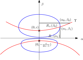
Figure 1. Figure 6.1

Case 3. $p_{1}$ $=$ $(\alpha_{1},\beta_{1})$ $\in$ $\Upsilon\backslash\{(0,c)\}$ $\cap$ (first quadrant). Since $\alpha^{\prime}$ $=$ $0$ and $\beta^{\prime}$ $<$ $0$ at $p_{1},$ the solution $p(s)$ to (6.3) with $p(s_{1})$ $=$ $p_{1}$ enters $R_{+}$ ($R_{-},$ resp.) for a small time interval $s_{1}$ $-$ $\varepsilon<$ $s<s_{1}$ ($s_{1}+\varepsilon$ $>$ $s$ $>$ $s_{1},$ resp.$)$.

Case 4. $p_{2}$ $=$ $(\alpha_{2},\beta_{2})$ $\in$ $R_{-}.$ Since $\alpha^{\prime}$ $<$ $0,$ $\beta^{\prime}$ $<$ $0$ in $R_{-},$ $\alpha(s)$ and $\beta(s)$ are increasing as $s$ changes towards the negative infinity, where $(\alpha(s),$ $\beta(s))$ $=$ $p(s)$ is the solution to (6.3) with $p(s_{2})$ $=$ $p_{2}$. Observe that

$$\beta^{\prime}(s) = -2n\beta(s)\alpha(s)$$

$$\leq -2n\beta(s_{2})\alpha(s_{2})<0$$

for $s$ $\leq$ $s_{2}.$ Suppose $p(s)$ does not hit $\Upsilon$ at any $s$ $<$ $s_{2}.$ Then $\beta(s)$ must go to $+\infty$ as $s$ $\rightarrow$ $-\infty.$ So there is $\tilde{s}_{2}$ $<$ $s_{2}$ such that $\beta(s)$ $\geq$ $2c$ for $s$ $\leq$ $\tilde{s}_{2}.$ Now from $\alpha^{\prime}$ $<$ $0$ and (6.3), we have

$$\alpha^{2} \geq \frac{1}{4n^{2}}(\beta-c)((2n-1)\beta+c)$$

$$\geq \frac{1}{4n^{2}}\frac{\beta}{2}((2n-1)\beta+c)$$

$$\geq \frac{2n-1}{8n^{2}}\beta^{2}.$$

It follows that $\alpha$ $\geq$ $c(n)\beta$ where $c(n)$ $=$ $\frac{\sqrt{2n-1}}{2\sqrt{2}n}.$ We can then estimate

$$-\beta^{\prime} = 2n\beta\alpha$$

$$\geq 2nc(n)\beta^{2}=\sqrt{n-\frac{1}{2}}\beta^{2}$$

which is reduced to $(\frac{1}{\beta})^{\prime}\geq\sqrt{n-\frac{1}{2}}.$ Integrating from $s$ to $\tilde{s}_{2}$ gives

(6.8) $$\frac{1}{\beta(\tilde{s}_{2})}-\frac{1}{\beta(s)}\geq\sqrt{n-\frac{1}{2}}(\tilde{s}_{2}-s).$$

As $s$ $\rightarrow$ $-\infty,$ the left hand side of (6.8) is bounded while the right hand side goes to $+\infty.$ The contradiction shows that $p(s)$ must hit $\Upsilon$ at some finite $\tilde{s}$ $<$ $s_{2}.$

On the other hand, consider the region $R_{-}(\alpha_{2})$ surrounded by $\Upsilon,$ $\alpha$ $=$ $\alpha_{2},$ $\beta$ $=$ $0$ ($\alpha$-axis), and the line segment $\{0\}$ $\times$ $[0,c]$ ($\alpha$ $=$ $0,$ $\ 0$ $\leq$ $\beta$ $\leq$ $c)$ (see Figure 6.1). Observe that the vector field $V$ (see 6.7) points inward (towards $R_{-}(\alpha_{2}))$ on $\Upsilon,$ $\alpha$ $=$ $\alpha_{2}$ while pointing outward on $\{0\}$ $\times$ $[0,c].$ Note that $V$ does not vanish in $R_{-}(\alpha_{2})$ and $\beta$ $=$ $0$ ($\alpha$-axis) is a solution to (6.3) with $\alpha^{\prime}=-\alpha^{2}+\frac{1}{4n^{2}}(-c^{2})$ $<$ $0.$ Therefore the solution curve $p(s)$ $:=$ $(\alpha(s),\beta(s))$ to (6.3) with $p(s_{2})=p_{2}$ must hit either some point in $\{0\}$ $\times$ $(0,c)$ at finite $\breve{s}_{2}$ $>$ $s_{2}$ or the point $(0,c)$ as $s\rightarrow+\infty$ by compactness of $\overline{R_{-}(\alpha_{2})}$ and uniqueness of ($C^{\infty}$ smooth) ODE solutions.

Next suppose $\lim_{s\rightarrow+\infty}p(s)$ $=$ $(0,c)$. We may assume $\beta$ $>$ $c$ (otherwise $\beta$ won’t tend to $c$ since $\beta$ is decreasing). From (6.3) we compute

$$\frac{d\alpha^{\prime}}{ds}$$

$$= -2\alpha\alpha^{\prime}+\frac{\beta^{\prime}}{4n^{2}}\{(2n-1)(\beta-c)+(2n-1)\beta+c\}$$

$$\leq 2\alpha^{3}-\frac{2n\beta\alpha}{4n^{2}}\{(2n-1)\beta+c\}\text{ (by }\beta^{\prime}<0\text{ and }\beta>c)$$

$$\leq 2\alpha^{3}-c^{2}\alpha.$$

Since lim${}_{s\rightarrow+\infty}\alpha(s)$ $=$ $0,$ we can find some large number $\breve{s}$ such that $\frac{d\alpha^{\prime}}{ds}$ $\leq$ $0$ for $s$ $\geq$ $\breve{s}$. It follows that $\alpha^{\prime}(s)$ $\leq$ $\alpha^{\prime}(\breve{s})$ $<$ $0.$ But $\lim_{s\rightarrow+\infty}\alpha^{\prime}(s)$ $=$ $0$ ($\alpha$ $\rightarrow$ $0,$ $\beta$ $\rightarrow$ $c).$ We have reached a contradiction. So we conclude that at finite $\breve{s}_{2}$ $>$ $s_{2}$, $p(\breve{s}_{2})$ $\in$ $\{0\}$ $\times$ $(0,c).$

Case 5. $p_{+}$ $\in$ $\{0\}$ $\times$ $(0,c).$ Observe that $\alpha^{\prime}$ $<$ $0$ and $\beta^{\prime}$ $=$ $0$ at $p_{+}.$ The solution $p(s)$ to (6.3) with $p(s_{+})$ $=$ $p_{+}$ will go into the second quadrant ($R_{-},$ resp.) for a short time after (before, resp.) $s_{+}.$

Altogether wherever in the first quadrant we start with, the solution ends up touching the $\beta$-axis in both finite negative and finite positive times. Then by the symmetry to the $\beta$-axis we obtain a closed periodic orbit.

(II) Suppose $p_{0}$ $=$ $(\alpha_{0},\beta_{0})$ $\in$ $R^{2,-}\backslash\{(0,-\frac{c}{2n-1})\}.$ Consider the transformation: $\tilde{\alpha}$ $=$ $\alpha,$ $\tilde{\beta}$ $=$ $-\beta.$ Then we have

(6.9) $$\tilde{\beta}^{\prime} = -2n\tilde{\beta}\tilde{\alpha}$$

$$\tilde{\alpha}^{\prime} = -\tilde{\alpha}^{2}+\frac{1}{4n^{2}}((2n-1)\tilde{\beta}-c)(\tilde{\beta}+c).$$

Since (6.9) for $\tilde{\beta}$ $>$ $0$ is similar to (6.3) for $\beta$ $>$ $0,$ we can analyze (6.9) similarly to get a periodic solution $(\tilde{\alpha}(s),$ $\tilde{\beta}(s))$ with $(\alpha_{0},-\beta_{0})$ as the initial data. Then $(\alpha(s),$ $\beta(s))$ $=$ $(\tilde{\alpha}(s),$ $-\tilde{\beta}(s))$ $\in$ $R^{2,-}\backslash\{(0,-\frac{c}{2n-1})\}$ is the required periodic solution. We have completed the proof.

   

To illustrate the result in Lemma 6.1, please see Figure 6.2 drawn by the computer.

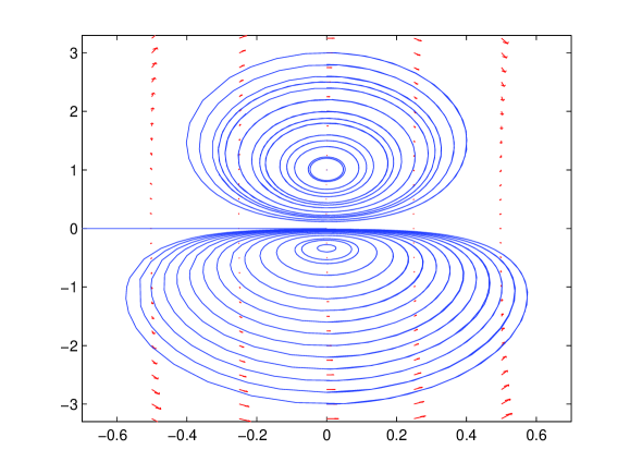
Figure 2. Figure 6.2: n=2, c=1

Proof.

(of Lemma B) Recall that $S_{\Sigma}$ denotes the set of singular points. For $K$ $\subset$ $\alpha\beta$-plane. we define the subset $\Sigma(K)$ $\subset$ $\Sigma\backslash S_{\Sigma}$ by

$$\Sigma(K)=\{p\in\Sigma\backslash S_{\Sigma}:(\alpha(p),\beta(p))\in K\}.$$

By Proposition 4.2 we obtain that $k,$ $l$ (and hence $\beta)$, and $\alpha$ are constant on each leaf of the ($2n-1$)-dimensional foliation described in Proposition 4.3. On the other hand, $e_{n}$ is transversal to the leaves by Proposition 4.3, hence $\Sigma(K)$ is open for $K$ $=$ $\{(0,c)\}$ or $\{(0,-\frac{c}{2n-1})\}$ or a periodic orbit in the $\alpha\beta$-plane, or the $\alpha$-axis by Lemma 6.1. It is also clear that $\Sigma(K)$ is a closed set for such a $K$. Note that $S_{\Sigma}$ consists of discrete (isolated singular) points by Proposition 4.1. So $\Sigma\backslash S_{\Sigma}$ is connected and identified with $\Sigma(K)$ if $\Sigma(K)$ $\neq$ $\emptyset$ since $\Sigma(K)$ is open and closed. Observe that $\alpha$ $\rightarrow$ $\pm\infty$ as regular points $p_{j}$ tend to a singular point. For $K$ $=$ $\{(0,c)\}$ or $\{(0,-\frac{c}{2n-1})\}$ or a periodic orbit in the $\alpha\beta$-plane, $\alpha$ is bounded. Therefore the only choice is $K$ $=$ $\alpha$-axis.(if there exists a singular point). That is, $0$ $=$ $\beta$ :$=$ $l-2k$ on $\Sigma\backslash S_{\Sigma}$.

   

7. Proof of Theorem A and beyond

Proof.

(of Theorem A) Suppose $\Sigma$ does not contain any singular point. Then $\Sigma$ is foliated by characteristic curves. Consider the line field defined by the tangent lines of characteristic curves. Then the Euler number is the index sum of this line field by Hopf’s index theorem ([19]). Since this line field never vanishes, the Euler number must be zero. This contradiction to the assumption shows the existence of a singular point. Next by Lemma B we have $l=2k$ on $\Sigma$. Then by Theorem 1.3, $\Sigma$ must be congruent with a Pansu sphere.

   

Another interesting problem is to relate level sets of a Sobolev extremal to umbilic hypersurfaces for different Sobolev exponents. Let

$$p^{\ast}:=\frac{pQ}{Q-p}$$

where $Q$ $=$ $2n+2,$ $p$ $\geq$ $1.$ The Sobolev inequality on $H_{n}$ reads

$$\parallel u\parallel_{L^{p^{\ast}}}\leq C\parallel\nabla_{b}u\parallel_{L^{p}}$$

for all functions $u$ such that both sides of the above inequality are finite. The best constant is obtained by minimizing the Sobolev quotient

$$\frac{\parallel\nabla_{b}u\parallel_{L^{p}}}{\parallel u\parallel_{L^{p^{\ast}}}}.$$

over all functions $u$ such that both $\parallel\nabla_{b}u\parallel_{L^{p}}$ and $\parallel u\parallel_{L^{p^{\ast}}}$ are finite and $\parallel u\parallel_{L^{p^{\ast}}}$ $\neq$ $0.$ The associated Euler-Lagrange equation reads

(7.1) $$\mathop{\mathrm{d}iv}_{b}(|\nabla_{b}u|^{p-2}\nabla_{b}u)=\sigma u^{p^{\ast}-1}$$

where $\sigma$ is a constant (Lagrange multiplier). For other interesting inequalities on $H_{n},$ the reader is referred to [10].

For $p$ $=$ $2,$ equation (7.1) is reduced to the $CR$ Yamabe equation

(7.2) $$\Delta_{b}u=\sigma u^{1+\frac{2}{n}}.$$

Observe that $u(z,t)$ $=$ $(4t^{2}+(|z|^{2}+\lambda)^{2})^{-n/2}$ with constant $\lambda$ $>$ $0$ is a solution to (7.2). The level sets of this solution are ”shifted” Heisenberg spheres $\Sigma_{\lambda}$ defined by $4t^{2}$ $+$ $(|z|^{2}+\lambda)^{2}$ $=$ $\rho_{0}^{4}.$ Although these are not Heisenberg spheres (see Example 3.3), they are still umbilic. Take

$$\varphi=\rho_{0}^{4}-[4t^{2}+(|z|^{2}+\lambda)^{2}]$$

as a defining function. Let $e_{2n}$ $:=$ $\frac{\nabla_{b}\varphi}{|\nabla_{b}\varphi|}$ (pointing inwards to the domain $\{\varphi$ $>$ $0\}$ at the boundary $\{\varphi$ $=$ $0\})$, $e_{n}$ $:=$ $-Je_{2n}$, and $e_{1},$ $..,e_{n-1},$ $e_{n+1},$ $..,$ $e_{2n-1}$ be an orthonormal frame of $\xi^{\prime}.$ Then it is not hard to compute $h_{jm}$ $=$ $0$ for $1$ $\leq$ $j,m$ $\leq$ $2n-1$ except $j$ $=$ $m$ and $|j-m|$ $=$ $n.$ Moreover, we have

(7.3) $$l = h_{nn}=\frac{2|z|^{2}+(|z|^{2}+\lambda)}{\rho_{0}^{2}|z|},$$

$$k = h_{jj}=\frac{|z|^{2}+\lambda}{\rho_{0}^{2}|z|},\text{ }1\leq j\leq 2n-1,j\neq n,$$

$$\alpha = \frac{2t}{\rho_{0}^{2}|z|}=h_{\beta(n+\beta)}=-h_{(n+\beta)\beta},\text{ }1\leq\beta\leq n-1.$$

From (7.3) we observe that $l$ $\leq$ $3k$ and

$$l=3k\iff\lambda=0\iff\Sigma_{\lambda}\text{ is a Heisenberg sphere.}$$

For $p=1,$ equation (7.1) is reduced to the following $p$-mean curvature equation

(7.4) $$H(=\mathop{\mathrm{d}iv}_{b}\frac{\nabla_{b}u}{|\nabla_{b}u|})=\sigma u^{\frac{1}{2n+1}}.$$

Observe that $H_{n}\backslash\{0\}$ $=$ $\cup_{0<\lambda<\infty}$ $S_{\lambda}$ where $S_{\lambda}$ is th Pansu sphere defined in (1.6). Define a function $u$ on $H_{n}\backslash\{0\}$ by $u$ $=$ $(\frac{2n\lambda}{\sigma})^{2n+1}$ on $S_{\lambda}.$ It is not hard to see that $u$ $\in$ $C^{2}(H_{n}\backslash\{0\})$ and (7.4) holds since, on $S_{\lambda},$ $H$ $=$ $2n\lambda$ (see Example 3.2) and $\sigma u^{\frac{1}{2n+1}}$ $=$ $2n\lambda$ too. So $u$ is a solution to (7.4) with umbilic level sets $S_{\lambda}.$ In this case, $l$ $=$ $2k.$ We would like to ask the following question for general $p$ $\geq$ $1:$

Question. Is each level set of a Sobolev extremal, solution to (7.1), umbilic?

References

- [1] Alexandrov, A. D., Uniqueness theorems for surfaces in the large I, Vestnik Leningrad Univ., 11 (1956) 5-17.
- [2] Cheng, J.-H. and Hwang, J.-F., Properly embedded and immersed minimal surfaces in the Heisenberg group, Bull. Aus. Math. Soc., 70 (2004) 507-520.
- [3] Cheng, J.-H. and Hwang, J.-F., Variations of generalized area functionals and p-area minimizers of bounded variation in the Heisenberg group, Bulletin of the Institute of Mathematics, Academia Sinica, New Series, 5 (2010) 369-412.
- [4] Cheng, J.-H. and Hwang, J.-F., Uniqueness of generalized -area minimizers and integrability of a horizontal normal in the Heisenberg group, Calc. Var. and PDE; http://arxiv.org/abs/1211.1474 (published online 2013).
- [5] Cheng, J.-H., Hwang, J.-F., Malchiodi, A., and Yang, P., Minimal surfaces in pseudohermitian geometry, Annali della Scuola Normale Superiore di Pisa, Classe di Scienze (5), 4 (2005) 129-177.
- [6] Cheng, J.-H., Hwang, J.-F., Malchiodi, A., and Yang, P., A Codazzi-like equation and the singular set for smooth surfaces in the Heisenberg group, Journal fur die reine und angewandte Mathematik, 671 (2012) 131-198.
- [7] Cheng, J.-H., Hwang, J.-F., and Yang, P., Existence and uniqueness for -area minimizers in the Heisenberg group, Math. Annalen, 337 (2007) 253-293.
- [8] Cheng, J.-H., Hwang, J.-F., and Yang, P., Regularity of smooth surfaces with prescribed -mean curvature in the Heisenberg group, Math. Annalen, 344 (2009) 1-35.
- [9] Chiu, H.-L. and Lai, S.-H., The fundamental theorem for hypersurfaces in Heisenberg groups, Cal. Var. and P.D.E., DOI 10.1007/s00526-015-0818-1, 2015.
- [10] Frank, R. L. and Lieb, E. H., Sharp constants in several inequalities on the Heisenberg group, Ann. of Math., 176 (2012) 349-381.
- [11] Lee, J. M., The Fefferman metric and pseudohermitian invariants, Trans. Amer. Math. Soc., 296 (1986) 411-429.
- [12] Lin, Y., and Ma, H., A characterization of spheres in the Heisenberg group preprint.
- [13] Montiel, S. and Ros, A., Compact hypersurfaces: the Alexandrov theorem for higher order mean curvatures, Diff. Geom., A symposium in honour of Manfredo do Carmo, Pitman Mono. and Surv. in Pure and Appl. Math. 52, ed. B. Lawson and K.Tenenblat, pp 279-296.
- [14] Pauls, S. D., Minimal surfaces in the Heisenberg group, Geometric Dedicata, 104 (2004) 201-231.
- [15] Pauls, S. D., H-minimal graphs of low regularity in Comment. Math. Helv. 81 (2006) 337-381; arXiv: math.DG/0505287 v3, Nov. 1, 2006 (to which the reader is referred).
- [16] Ritoré, M., Examples of area-minimizing surfaces in the subriemannian Heisenberg group with low regularity, Calc. Var. and PDE (2008), doi:10.1007/s00526-008-0181-6
- [17] Ritoré, M., A proof by calibration of an isoperimetric inequality in the Heisenberg group , Calc. Var. and PDE, 44 (2012) 47-60.
- [18] Ritoré, M. and Rosales, C., Area-stationary surfaces in the Heisenberg group Advances in Math., 219 (2008) 633-671.
- [19] Spivak, M., A comprehensive introduction to differential geometry, Vol. 3, Publish or Perish, Inc., Boston, 1975.
- [20] Webster, S. M., Pseudohermitian structures on a real hypersurface, J. Diff. Geom. 13 (1978) 25-41.