Point visibility graph recognition is NP-hard

Abstract

Given a 3-SAT formula, a graph can be constructed in polynomial time such that the graph is a point visibility graph if and only if the 3-SAT formula is satisfiable. This reduction establishes that the problem of recognition of point visibility graphs is NP-hard.

Bodhayan Roy School of Technology and Computer Science Tata Institute of Fundamental Research Mumbai 400005, India bodhayan@tifr.res.in

1 Introduction

The visibility graph is a fundamental structure studied in the field of computational geometry and geometric graph theory [2, 5]. Some of the early applications of visibility graphs included computing Euclidean shortest paths in the presence of obstacles [9] and decomposing two-dimensional shapes into clusters [12]. Here, we consider problems from visibility graph theory. Let $P=\{p_{1},p_{2},...,p_{n}\}$ be a set of $n$ points in the plane. We say that two points $p_{i}$ and $p_{j}$ of $P$ are visible to each other if the line segment $p_{i}p_{j}$ does not contain any other point of $P$. In other words, $p_{i}$ and $p_{j}$ are visible to each other if $P\cap{p_{i}p_{j}}=\{p_{i},p_{j}\}$. If two points are not visible, they are called invisible to each other. If a point $p_{k}\in P$ lies on the segment $p_{i}p_{j}$ connecting two points $p_{i}$ and $p_{j}$ in $P$, we say that $p_{k}$ blocks the visibility between $p_{i}$ and $p_{j}$, and $p_{k}$ is called a blocker in $P$. The point visibility graph (denoted as PVG) of $P$ is defined by associating a vertex $v_{i}$ with each point $p_{i}$ of $P$ and an undirected edge $(v_{i},v_{j})$ of the PVG if $p_{i}$ and $p_{j}$ are visible to each other. Observe that if no three points of $P$ are collinear, then the PVG is a complete graph as each pair of points in $P$ is visible since there is no blocker in $P$. Point visibility graphs have been studied in the context of connectivity [10], chromatic number and clique number [8, 11]. For review and open problems on point visibility graphs, see Ghosh and Goswami [6]. Given a point set $P$, the PVG of $P$ can be computed in polynomial time. Using the result of Chazelle et al. [1] or Edelsbrunner et al. [4], this can be achieved in $O(n^{2})$ time. Consider the opposite problem: given a graph $G$, determine if there is a set of points $P$ whose point visibility graph is $G$. This problem is called the point visibility graph recognition problem [6]. Identifying the set of properties satisfied by all visibility graphs is called the point visibility graph characterization problem. The problem of actually drawing one such set of points $P$ whose point visibility graph is the given graph $G$, is called the point visibility graph reconstruction problem. Such a point set itself is called a visibility embedding of $G$. Ghosh and Roy [7] presented a complete characterization for planar point visibility graphs, which leads to a linear time recognition and reconstruction algorithm. For recognizing arbitrary point visibility graphs, they presented three necessary conditions, and gave a polynomial time algorithm for testing the first necessary condition. However, it is not clear whether the other two necessary conditions can be checked in polynomial time. If a set of necessary and sufficient conditions for recognizing point visibility graphs can be found such that they can be tested in polynomial time, then the recognition problem lies in P. So, it is necessary to investigate the complexity issues of recognizing point visibility graphs. This problem is known to be in PSPACE, which is the only upper bound known on the complexity of the problem [7, 6]. On the other hand, problems of minimum vertex cover, maximum independent set, and maximum clique of point visibility graphs are shown to be NP-hard [7, 6]. In this paper, we show that the recognition problem for $PVGs$ is NP-hard. In Section 2, we develop a slanted grid graph (denoted as $SGG$) that has a unique visibility embedding. The embedding of the $SGG$ contains a gridlike structure. In Section 3, we transform the slanted grid graph into a modified slanted grid graph (denoted as $MSGG$), that also has a unique visibility embedding. The unique visibility embedding of the $MSGG$ also contains a gridlike structure, however, an area inside the grid is devoid of points. This area is later used to embed another graph inside the $MSGG$. In Section 3.1 we describe the construction of the $MSGG$. In Section 3.2 we begin with lemmas on some less complex graphs and finally prove that the $MSGG$ has a unique visibility embedding. In Section 4 we first introduce a 3-SAT graph, that has vertices and edges corresponding to a given 3-SAT formula and its size polynomial in the size of the given 3-SAT formula. We describe the construction of the 3-SAT graph in Section 4.1. In Section 4.2, we strategically add this graph to a large enough $MSGG$, and call the result a reduction graph. The reduction graph inherits collinearity conditions from the $MSGG$, so that if it has a visibility embedding, then the configuration of its points belonging to the 3-SAT graph corresponds to a truth assignment of the given 3-SAT formula. In Section 4.2, we prove that if the given 3-SAT formula is not satisfiable, then the reduction graph has no visibility embedding. In Section 4.4, we prove the converse direction of the reduction, i.e., that if the given 3-SAT formula is satisfiable, then the reduction graph has a visibility embedding. This completes the reduction. In Section 5, we conclude the paper with a few remarks.

2 Slanted grid graphs

In this section, we define a special type of $PVG$ called the slanted grid graph ($SGG$). Intuitively, an $SGG$ is a $PVG$ resembling a grid graph [3] with two extra vertices so that in its visibility embedding, every line passes through at least one of these two vertices. These two extra vertices are called vertices of convergence. Let $G=(V,E)$ be the $PVG$ of a point set $P$. Let $f:V\longrightarrow P$ be a bijection. We say that the pair $\langle P,f\rangle$ is a visibility embedding of $G$ if

$$P\cap p_{i}p_{j}=\{p_{i},p_{j}\}\Longleftrightarrow(f^{-1}(p_{i}),f^{-1}(p_{j}))\in E\enspace.$$

Let $G_{0}=(V_{0},E_{0})$ be a PVG, and $\xi=\langle\{p_{1},p_{2},...,p_{n}\},f\rangle$ and $\xi^{\prime}=\langle\{p_{1}^{\prime},p_{2}^{\prime},...,p_{n}^{\prime}\},f^{\prime}\rangle$ be two visibility embeddings of $G_{0}$. A line passing through some points of $\xi$ is simply referred to as a line in $\xi$. Let $L$ be a line in $\xi$ and let $\langle p_{i_{1}},p_{i_{2}},...,p_{i_{\ell}}\rangle$ be the sequence of all points in $\xi$ that lie on $L$ in this order. We say that $L$ is preserved in $\xi^{\prime}$ if all the points in the sequence $L^{\prime}=\langle f^{\prime}(f^{-1}(p_{i_{1}})),f^{\prime}(f^{-1}(p_{i_{2}})),...,f^{\prime}(f^{-1}(p_{i_{\ell}}))\rangle$ lie on the same line, in the same order and no other point of $\xi^{\prime}$ lies on $L^{\prime}$.

Let $m\in\mathbb{N}$ and $n\in\mathbb{N}$ be two numbers such that $m\geq 3$ and $n\geq 3$. Consider graph $G_{0}=(V_{0},E_{0})$, where $V_{0}$ and $E_{0}$ are defined as follows.

$$V_{0} = \{v_{i,j}|1\leq i\leq n\textrm{ and }1\leq j\leq m\}\cup\{v_{1},v_{2}\}$$

$$E_{0} = \{(v_{i,j},v_{k,l})|i\neq k\textrm{ and }j\neq l\}\cup\{(v_{1},v_{1,j})|1\leq j\leq m\}\cup\{(v_{2},v_{i,1})|1\leq i\leq n\}\cup\{(v_{1},v_{2})\}$$

$$\cup \{(v_{i,j},v_{i+1,j})|1\leq i\leq n-1\textrm{ and }1\leq j\leq m\}\cup\{(v_{i,j},v_{i,j+1})|1\leq i\leq n\textrm{ and }1\leq j\leq m-1\}$$

Observe that $|V_{0}|=mn+2$ and $|E_{0}|=(mn-m-n+3)mn+1$. We call this graph a slanted grid graph (SGG), which is a $PVG$ with visibility embedding as explained below. Consider a set of points

$$P=\{p_{i,j}|1\leq i\leq n\textrm{ and }1\leq j\leq m\}\cup\{p_{1},p_{2}\}$$

and associate $v_{1}$ to $p_{1}$, $v_{2}$ to $p_{2}$ and $v_{i,j}$ to $p_{i,j}$ for $1\leq i\leq n$ and $1\leq j\leq m$. A line passing through exactly two embedding points of $P$ is called an ordinary line. A line passing through three or more embedding points of $P$ is called a non-ordinary line. Choose the coordinates of the points in $P$ in such a way that the non-ordinary lines in $P$ contain $\langle p_{1},p_{1,j},p_{2,j},...,p_{n,j}\rangle$ for $1\leq j\leq m$ and $\langle p_{2},p_{i,1},p_{i,2},...,p_{i,m}\rangle$ for $1\leq i\leq n$ (Figure 1). Then $P$ is a visibility embedding of $G_{0}$, and points of $P$ are referred to as embedding points.

In the following lemma, we prove that this visibility embedding is actually unique, up to the preservation of the lines.

Figure 1: Visibility embedding of a slanted grid graph. The graph contains $mn+2$ vertices and $(mn-m-n+3)mn+1$ edges.

Lemma 1.

$G_{0}$ has a unique visibility embedding, up to the preservation of lines (Figure 1).

Proof.

Suppose that the embedding points $\{p_{1,1},p_{2,1},\ldots,p_{n,1}\}$ lie on both sides of $\overleftarrow{p_{2}p_{1}}$. Let $p_{x,1}$ and $p_{y,1}$ be the embedding points from $\{p_{1,1},p_{2,1},\ldots,p_{n,1}\}$ such that $\overleftarrow{p_{2}p_{x,1}}$ and $\overleftarrow{p_{2}p_{y,1}}$ make the smallest angles with $\overleftarrow{p_{2}p_{1}}$ to its left and right respectively. Now, only one embedding point among $p_{x,1}$ and $p_{y,1}$ (say, $p_{x,1}$) can be $p_{1,1}$. So, some point $p_{a,b}$ must block $p_{y,1}$ from $p_{1}$. But then $\overleftarrow{p_{2}p_{a,b}}$ forms a smaller angle than $\overleftarrow{p_{2}p_{y,1}}$ with $\overleftarrow{p_{2}p_{1}}$ on the same side, a contradiction. Therefore, embedding points of $\{p_{1,1},p_{2,1},\ldots,p_{n,1}\}$, and the remaining embedding points of $P$ must lie on the same side of $\overleftarrow{p_{2}p_{1}}$. Since $p_{1}$ and $p_{2}$ are mutually visible, no other embedding point can lie on $\overline{p_{1}p_{2}}$. Consider an embedding point of $\{p_{1,1},p_{2,1},\ldots,p_{n,1}\}$ lying on $\overleftarrow{p_{1}p_{2}}$. Since the consecutive embedding points of $\{p_{1},p_{1,1},p_{2,1},\ldots,p_{n,1}\}$ are all visible to each other and all of them are visible from $p_{2}$, and $n\geq 3$, they must either be collinear or form a reflex chain facing $p_{2}$. In either of these two cases, none of the embedding points of $\{p_{1,1},p_{2,1},\ldots,p_{n,1}\}$ lies on $\overleftrightarrow{p_{1}p_{2}}$. Since $m\geq 3$, an analogous reasoning shows that none of the embedding points of $\{p_{1,1},p_{1,2},\ldots,p_{1,m}\}$ lies on $\overleftrightarrow{p_{1}p_{2}}$. Hence, no remaining point of $P$ lies on $\overleftrightarrow{p_{1}p_{2}}$. There are $m+1$ and $n+1$ vertices in $G_{0}$ adjacent to $v_{1}$ and $v_{2}$ respectively. So there are $m+1$ and $n+1$ rays originating from $p_{1}$ and $p_{2}$ in a visibility embedding of $G_{0}$ respectively. Consider the line passing through $p_{1}$ and $p_{2}$. We leave aside the two rays from $p_{1}$ and $p_{2}$ because we have proved that no remaining point of $P$ lies on $\overleftrightarrow{p_{1}p_{2}}$. Observe that embedding points can only be placed on the possible intersection points of the remaining rays. There are at most $m\times n$ intersection points formed by the remaining rays. However, since there are $m\times n$ remaining vertices of $G_{0}$, there are exactly $m\times n$ intersection points formed by the remaining rays. We call this configuration a slanted grid. Observe that neither $p_{1}$ nor $p_{2}$ can be placed inside the convex hull of the other points, because otherwise either not all embedding points lie on the same side of $\overleftarrow{p_{2}p_{1}}$, or some other embedding point lies on $\overleftrightarrow{p_{1}p_{2}}$, a contradiction. Wlog we assume that $p_{1}$ is placed to the right of all other points, and $p_{2}$ is placed above all the other points (see Figure 1). For convenience, we refer to the rays from $p_{1}$ as horizontal and the rays from $p_{2}$ as vertical. Hence, the embedding points can only permute their positions on the intersection points of rays.

Since $\{v_{1,1},v_{2,1},\ldots,v_{n,1}\}$ are adjacent to $v_{2}$, the embedding points $\{p_{1,1},p_{2,1},\ldots,p_{n,1}\}$ must occur on the topmost horizontal ray from $p_{1}$. Since $v_{1,1}$ is adjacent to $v_{1}$, $p_{1,1}$ must be embedded to the left of $p_{1}$ with no other embedding point on $p_{1,1}p_{1}$. For $1\leq i\leq n-1$, $v_{i+1,1}$ is adjacent to $v_{i,1}$, and therefore, $p_{i+1,1}$ must be embedded to the left of $p_{i,1}$ with no other embedding point on $p_{i+1,1}p_{i,1}$. Hence, the topmost horizontal line is preserved. Since the vertices $\{v_{1,2},v_{2,2},\ldots,v_{n,2}\}$ are the only vertices other than $v_{2}$ adjacent to all the vertices $\{v_{1,1},v_{2,1},\ldots,v_{n,1}\}$, $\{p_{1,2},p_{2,2},\ldots,p_{n,2}\}$ must occur on the second-topmost horizontal ray from $p_{1}$. By applying the previous reasoning, the second-topmost horizontal line is also preserved. Similar arguments hold for other horizontal and vertical rays. ∎

Figure 2: An embedding of the $SGG$ after deletion of vertices.

Figure 3: Visibility embedding of a modified slanted grid graph. $G^{\prime}$ is not a part of the MSGG.

3 Modified slanted grid graphs

In a visibility embedding of an $SGG$, every intersection point contains an embedding point. However, if we delete some embedding points (Figure 2), then it is not clear whether the visibility graph of the remaining point set has a unique visibility embedding. In order to ensure a unique embedding after deletion, some new vertices are added to $G_{0}$ which facilitate a unique visibility embedding of the resulting graph $G$. In general, the vertices are added such that in every embedding there are four lines passing through a large number of embedding points, that enforce certain collinearity conditions and result in a unique visibility embedding up to the preservation of lines.

3.1 Construction of a modified slanted grid graph

Consider the unique embedding $\xi$ of a slanted grid graph $G_{0}$ with $n\times n$ embedding points and the two embedding points of convergence. We construct a modified slanted grid graph (denoted as $MSGG$) $G(V,E)$ by adding some vertices to $G_{0}$ and then deleting some other vertices from it. We now describe the modification of $G_{0}$. Let $G_{0}$ be the $SGG$ on $(n\times n)+2$ vertices defined in the previous section. Consider a positive intger $m_{0}$, $m_{0}\leq n-2$. Note that the removal of vertices from $V$ also implies the removal of their incident edges from $E$. We make the following modifications in $G_{0}$ to construct $G$.

$$V = (V_{0}\setminus\{v_{i,j}|n-m_{0}+1\leq i\leq n\textrm{ and }3\leq j\leq n\})\cup\{v_{i,j}|n+1\leq i\leq 2n^{4}-n\textrm{ and }1\leq j\leq 2\}$$

$$\cup\{v_{i,j}|1\leq i\leq 2\textrm{ and }n+1\leq j\leq 25n^{8}+n\}$$

$$E = E_{0}\cup\{(v_{i,j},v_{i-1,j})|n+1\leq i\leq 2n^{4}+n\textrm{ and }1\leq j\leq 2\}$$

$$\cup\{(v_{i,1},v_{j,2})|1\leq i,j\leq 2n^{4}+n\}$$

$$\cup\{(v_{i,j},v_{k,l})|n+1\leq i\leq 2n^{4}+n\textrm{ and }1\leq j\leq 2\textrm{ and }1\leq k\leq n-m_{0}\textrm{ and }3\leq l\leq n\}$$

$$\cup\{(v_{i,j-1},v_{i,j})|1\leq i\leq 2\textrm{ and }n+1\leq j\leq 25n^{8}+n\}$$

$$\cup\{(v_{1,i},v_{2,j})|1\leq i,j\leq 25n^{8}+n\}$$

$$\cup\{(v_{i,j},v_{k,l})|1\leq i\leq 2\textrm{ and }n+1\leq j\leq 25n^{8}+n\textrm{ and }3\leq k\leq n-m_{0}\textrm{ and }1\leq l\leq n\}$$

$$\cup\{(v_{i,j},v_{k,l})|1\leq j,k\leq 2\textrm{ and }3\leq i\leq 2n^{4}+n\textrm{ and }3\leq l\leq 25n^{8}+n\}$$

Intuitively the $m_{0}(n-2)$ vertices that are deleted correspond to an $m_{0}\times(n-2)$ grid in the visibility embedding of $G$. Since $m_{0}\leq n-2$, the vertices of $L_{1}$ and $L_{2}$ are not deleted. If $m_{0}^{2}$ vertices are later added to the graph with suitable adjacency relationships, then they can be forced to be embedded on particular horizontal lines (see the proof of Lemma 9). Now we construct a visibility embedding of the modified $G$, from the initial unique visibility embedding of $G$ in Figure 1. Let $L_{1}$ and $L_{2}$ be the rightmost and second-rightmost lines of the visibility-embedding of an $MSGG$ (Figure 3). Let $L_{3}$ and $L_{4}$ be the topmost and second-topmost lines of the visibility-embedding of an $MSGG$. The bottommost horizontal line and leftmost vertical line are labelled $L_{5}$ and $L_{6}$, respectively. As shown in Figure 3, the two points of convergence are above and to the right of the embedding. As before, $p_{i,j}$ is the embedding point corresponding to the vertex $v_{i,j}$.

1. Delete the $(n-2)\times m_{0}$ bottom-left subgrid of $G$ (See Figure 2). At a later stage, we embed a gadget in the space thus created.

2. To the left of $L_{6}$, place $2n^{4}$ embedding points on $L_{4}$, and $2n^{4}$ embedding points on $L_{3}$ (See Figure 3). These embedding points must be placed in such a way that $(a)$ each embedding point added to $L_{3}$ blocks an embedding point on $L_{4}$ from $p_{2}$, $(b)$ each embedding point added on $L_{3}$ sees every embedding point of $G$ not on $L_{3}$, and $(c)$ each embedding point added on $L_{4}$ sees every embedding point of $G$ not on $L_{4}$. To achieve this, the embedding points on $L_{4}$ and $L_{3}$ are added by considering the intersections of $L_{3}$ and $L_{4}$ with lines containing the edges of $G$. Such intersections are at most twice the number of edges in $G$. Each new embedding point can be placed on $L_{4}$ and its blocker on $L_{3}$ by avoiding these intersections. Add all edges between embedding points that are visible to each other.

3. Below $L_{5}$, place $25n^{8}$ embedding points on $L_{2}$, and $25n^{8}$ embedding points on $L_{1}$ (See Figure 3). These embedding points must be placed in such a way that $(a)$ each embedding point added to $L_{1}$ blocks an embedding point on $L_{2}$ from $p_{1}$, $(b)$ each embedding point added on $L_{1}$ sees every embedding point of $G$ not on $L_{1}$, and $(c)$ each embedding point added on $L_{2}$ sees every embedding point of $G$ not on $L_{2}$. To achieve this, the embedding points are added by following the method in step 2. Add all edges between embedding points that are visible to each other.

Henceforth $G$ is referred to as the modified slanted grid graph, denoted as $MSGG$. Observe that for all pairs of embedding points $p_{i,j}$ and $p_{k,l}$ where $i\neq k$ and $j\neq l$, $p_{i,j}$ and $p_{k,l}$ are mutually visible.

3.2 Unique visibility embedding of MSGG

Here we prove that every $MSGG$ has only one visibility embedding, unique up to the preservation of lines. We start with a few properties.

Figure 4: (a) The point $p_{i}$ is on $L$ and hence sees at most $l+2$ embedding points. (a) The point $p_{i}$ is not on $L$ and hence sees at least $k$ embedding points.

Lemma 2.

Let $H_{1}$ be a $PVG$ with visibility embedding $\xi$. Let $L$ be a line in $\xi$ such that $(i)$ there are $k$ embedding points on $L$, and $(ii)$ $l$ embedding points not on $L$. Let $v_{i}$ be a vertex of $H_{1}$ and $p_{i}$ its corresponding embedding point in $\xi$. If $p_{i}$ lies on $L$, then $deg(v_{i})\leq l+2$. Otherwise, $deg(v_{i})\geq k$.

Proof.

If $p_{i}$ lies on $L$ then $p_{i}$ sees at most two embedding points on $L$, and at most all $l$ embedding points that are not on $L$ (see Figure 4(a)). If $p_{i}$ does not lie on $L$, then all $k$ embedding points on $L$ lie on distinct lines passing through $p_{i}$. So, $p_{i}$ sees at least $k$ embedding points (see Figure 4(b)). ∎

Lemma 3.

Let $H_{2}$ be a $PVG$ with visibility embedding $\xi$. Let $L$ be a line in $\xi$ such that $(i)$ there are $k$ embedding points on $L$, and $(ii)$ $l$ embedding points not on $L$. If $k\geq(l+3)^{2}$ then $L$ is preserved in every visibility embedding of $H_{2}$ (Figure 5(a)).

Proof.

By the hypotheses, $H_{2}$ has $k+l$ vertices. Let us assume on the contrary that $L$ is not preserved in some visibility embedding $\xi^{\prime}$ of $H_{2}$. Let $\phi$ denote the bijection between $\xi$ and $\xi^{\prime}$. Let $\phi(L)$ denote the set of images of all embedding points lying on $L$, in $\xi^{\prime}$. We have the following cases depending on the collinearity of the embedding points of $\phi(L)$. Case 1: All embedding points in $\phi(L)$ are collinear. Case 2: Not all embedding points in $\phi(L)$ are collinear. Consider Case 1. Let $L^{\prime}$ be the line containing all embedding points of $\phi(L)$. Consider the situation where $L^{\prime}$ contains only the embedding points of $\phi(L)$. Let $p_{i-1}$, $p_{i}$ and $p_{i+1}$ be three consecutive embedding points on $L$ whose corresponding vertices in $H_{2}$ are $v_{i-1}$, $v_{i}$ and $v_{i+1}$ respectively. Clearly, $\phi(p_{i-1})$, $\phi(p_{i})$ and $\phi(p_{i+1})$ must be consecutive embedding points on $L^{\prime}$, since $(v_{i-1},v_{i})$ and $(v_{i},v_{i+1})$ are edges of $H_{2}$. A similar argument holds for the first and last embedding points of $L^{\prime}$. Hence, $L$ is preserved. Consider the other situation where $L^{\prime}$ contains an embedding point $p_{i}$ not in $\phi(L)$. Let the corresponding vertex to $p_{i}$ in $H_{2}$ be $v_{i}$. Since $p_{i}\notin L$ and $\phi(p_{i})$ lies on $L^{\prime}$, $k\leq deg(v_{i})\leq l+2$ by Lemma 2, contradicting the assumption that $k\geq(l+3)^{2}$. Consider Case 2. If not all embedding points of $\phi(L)$ are collinear, then either $(i)$ no $(l+3)$ embedding points of $\phi(L)$ are collinear, or $(ii)$ some $(l+3)$ embedding points of $\phi(L)$ are collinear . Consider $(i)$. Let $p_{i}\in\phi(L)$. Since $|\phi(L)|\geq(l+3)^{2}$ by assumption and no $(l+3)$ embedding points of $\phi(L)$ are collinear, there are at least $(l+4)$ distinct lines passing through $p_{i}$. So, the degree of the corresponding vertex $v_{i}$ of $p_{i}$ in $H_{2}$ is at least $(l+4)$. On the other hand, by Lemma 2, $deg(v_{i})\leq l+2$, a contradiction. Consider $(ii)$. Let $L^{\prime}$ be a line containing $(l+3)$ embedding points of $\phi(L)$. Let $p_{i}\in\phi(L)$ and $p_{i}\notin L^{\prime}$ such that $p_{i}$ is closest to $L^{\prime}$ among all embedding points of $\phi(L)$. Since $\phi^{-1}(p_{i})$ sees at most two points on $L$, $p_{i}$ does not see at least $l+1$ points. Hence, $p_{i}$ requires $l+1$ blockers where no blocker is from $\phi(L)$ by the choice of $p_{i}$. On the other hand, there are only $l$ points not in $\phi(L)$, a contradiction. ∎

Let $L_{a}$ and $L_{b}$ be two lines in a visibility embedding $\xi$ of a special type of PVG such that most of the embedding points of $\xi$ are on $L_{a}$ and $L_{b}$ (Figure 5(b)). In the following lemma, we show that $L_{a}$ and $L_{b}$ are preserved in every visibility embedding of the PVG.

Figure 5: (a) The line $L$ is preserved. (b) Both lines $L_{a}$ and $L_{b}$ are preserved.

Lemma 4.

Let $H_{3}$ be a PVG with visibility embedding $\xi$. Let $L_{a}=\langle p_{1},p_{2},...,p_{k}\rangle$, and $L_{b}=\langle p_{1},p_{k+1},...,p_{2k-1}\rangle$ be two lines in $\xi$ such that $k\geq(l+3)^{2}$, where $l$ denotes the number of embedding points in $\xi\setminus\{L_{a}\cup L_{b}\}$. Let $p_{2k}$ be an embedding point satisfying the following properties.

1. The embedding point $p_{2k}$ is adjacent to all embedding points in $L_{b}$, and is not adjacent to any other embedding point of $\xi$.

2. For $1<i\leq k$, $p_{k+i-1}$ blocks $p_{i}$ from $p_{2k}$ .

3. Every embedding point in $L_{a}\setminus\{p_{1}\}$ is adjacent to every embedding point in $L_{b}\setminus\{p_{1}\}$.

4. No embedding point in $\xi\setminus(L_{a}\cup L_{b}\cup\{p_{2k}\})$ is adjacent to any embedding point of $L_{b}$.

Then $L_{a}$ and $L_{b}$ are preserved in every visibility embedding of $H_{3}$, and the embedding points in $\xi\setminus(L_{a}\cup L_{b}\cup\{p_{2k}\})$ lie outside the convex hull of $(L_{a}\cup L_{b}\cup\{p_{2k}\})$.

Proof.

Let $\xi^{\prime}$ be any other visibility embedding of $H_{3}$. Let $\phi$ denote the bijection between $\xi$ and $\xi^{\prime}$. So, $\phi(L_{a})$ and $\phi(L_{b})$ are the images of $L_{a}$ and $L_{b}$ in $\xi^{\prime}$, respectively. We know that embedding points of $\phi(L_{b})$ are adjacent to $\phi(p_{2k})$. The order of embedding points along $\phi(L_{b})$ must be the same as that of $L_{b}$, because otherwise, the corresponding edges in the PVGs for $\xi$ and $\xi^{\prime}$ are different, a contradiction. Consider any three consecutive points $\phi(p_{i})$, $\phi(p_{i+1})$ and $\phi(p_{i+2})$ of $\xi^{\prime}$ on $\phi(L_{b})$ (Figure 6(a)). If $\phi(p_{i+1})$ is the blocker between $\phi(p_{i})$ and $\phi(p_{i+2})$, then they are collinear. Otherwise, consider the triangle $\phi(p_{i})\phi(p_{i+2})\phi(p_{2k})$. Observe that $\phi(p_{i})\phi(p_{i+2})\phi(p_{2k})$ must be a triangle and not a line segment with $\phi(p_{2k})$ in the middle, for otherwise, the points of $\phi(L_{b})\setminus\{\phi(p_{i})$, $\phi(p_{i+1})$ and $\phi(p_{i+2}\}$, which are all visible from $\phi(p_{2k})$ must lie outside of segment $\phi(p_{i})\phi(p_{2k})\phi(p_{i+2})$. Hence, they must be blocked from $\phi(p_{i})$ or $\phi(p_{i+2})$. Clearly, there are not enough blockers to achieve this, hence forcing $\phi(p_{i})\phi(p_{i+2})\phi(p_{2k})$ to be a triangle. If $\phi(p_{i+1})$ lies inside the triangle, then some point from $\xi^{\prime}\setminus(\phi(L_{b})\cup\{\phi(p_{2k})\})$ can block $\phi(p_{i})$ and $\phi(p_{i+2})$. Consider the other case where $\phi(p_{i+1})$ lies outside the triangle. The blocker between $\phi(p_{i})$ and $\phi(p_{i+2})$ must be adjacent to $\phi(p_{2k})$, and only the points of $\phi(L_{b})$ are adjacent to $\phi(p_{2k})$. If points from $\phi(L_{b})$ act as blockers between $\phi(p_{i})$ and $\phi(p_{i+2})$, the blockers must form a chain where consecutive points see each other. If other points from $\phi(L_{b})$ are used as blockers, then this chain is broken at some point. So, there cannot be any blocker of $\phi(p_{i})$ and $\phi(p_{i+2})$. Hence, the points of $\phi(L_{b})$ must either be collinear or form a reflex chain facing $\phi(p_{2k})$ (Figure 6(b)). Before showing that $L_{b}$ is preserved, we show that $L_{a}$ is preserved. Since the embedding points of $\phi(L_{b})$ form a reflex chain or a straight line and they are the only embedding points adjacent to $\phi(p_{2k})$, no embedding point of $(\phi(L_{b})\cup\{\phi(p_{2k})\})$ can be a blocker for any pair of the remaining embedding points of $\xi^{\prime}$. In addition, these embedding points are also not blockers between $\phi(p_{1})$ and any other embedding point of $\xi^{\prime}$. So, applying Lemma 3 on $(\xi^{\prime}\setminus((\phi(L_{b})\setminus\{\phi(p_{1})\})\cup\{\phi(p_{2k})\}))$, we get that $L_{a}$ is preserved. Since $L_{a}$ is preserved and $|\phi(L_{a})|=|\phi(L_{b})|$, the embedding points of $\phi(L_{a})$ cannot be blockers for pairs of embedding points of $\phi(L_{b})$. Observe that as no embedding point of $p_{q}\in(\xi^{\prime}\setminus\{\phi(L_{a})\cup\phi(L_{b})\cup\{\phi(p_{2k})\}\})$ is visible from $\phi(p_{2}k)$, if they lie inside the region bounded by $\phi(L_{a})$ and $\phi(L_{b})$, then they must lie on rays from $\phi(p_{2}k)$ passing through points of $\phi(L_{a})$. This blocks points of $\phi(L_{a})$ and $\phi(L_{b})$ from each other. So, no embedding point $p_{q}\in(\xi^{\prime}\setminus\{\phi(L_{a})\cup\phi(L_{b})\cup\{\phi(p_{2k})\}\})$ can lie inside the region bounded by $\phi(L_{a})$ and $\phi(L_{b})$. Therefore, $p_{q}$ cannot be a blocker for pairs of embedding points of $\phi(L_{b})$. Hence, the blockers for embedding points of $\phi(L_{b})$ must come from $\phi(L_{b})$ itself. So, the points of $\phi(L_{b})$ are collinear and $L_{b}$ is preserved. ∎

Figure 6: (a) In $\xi^{\prime}$, $\phi(L_{b})$ is not a reflex chain. (b) In $\xi^{\prime}$, $\phi(L_{b})$ a reflex chain facing $\phi(p_{2k})$.

Lemma 5.

Let $G$ be a modified slanted grid graph with visibility embedding $\xi$ (Figure 3). Let $L_{1}$ and $L_{2}$ be the rightmost and the second-rightmost lines in $\xi$, respectively. Let $L_{3}$ and $L_{4}$ be the topmost and the second-topmost lines in $\xi$, respectively. The lines $L_{1}$, $L_{2}$, $L_{3}$ and $L_{4}$ are preserved in every visibility embedding of $G$.

Proof.

Let $\xi^{\prime}$ be any other visibility embedding of $G$. Let $\phi$ denote the bijection between $\xi$ and $\xi^{\prime}$. So, $\phi(L_{1})$, $\phi(L_{2})$, $\phi(L_{3})$ and $\phi(L_{4})$ are the images of $L_{1}$, $L_{2}$, $L_{3}$ and $L_{4}$ in $\xi^{\prime}$, respectively. First we show that $L_{1}$ and $L_{2}$ are preserved. $\phi(L_{1})\setminus\{\phi(p_{2})\}$ and $\phi(L_{2})\setminus\{\phi(p_{2})\}$ contain $25n^{8}+n$ embedding points each by construction and $\xi^{\prime}\setminus(\phi(L_{1})\cup\phi(L_{2}))$ contains at most $4n^{4}+n^{2}-2n-m_{0}^{2}+1$ embedding points by construction, where $1\leq\ m_{0}\leq n-2$. Observe that $25n^{8}+n+1\geq(4n^{4}+n^{2}-2n-m_{0}^{2}+4)^{2}$ for large $n$. Since $k\geq(l+3)^{2}$, where $k=25n^{8}+n+1$ and $l=4n^{4}+n^{2}-2n-m_{0}^{2}+1$, both $L_{1}$ and $L_{2}$ are preserved by Lemma 4. Now we show that $L_{3}$ and $L_{4}$ are preserved. Let us start by identifying the partition of blockers in $\xi^{\prime}$ with respect to $\phi(L_{1})$ and $\phi(L_{2})$. Without loss of generality, let $\phi(p_{2})$ be the topmost embedding point, $\phi(L_{1})$ be to the right of $\phi(L_{2})$ and $\phi(p_{1})$ be to the right of $\phi(L_{1})$ in $\xi^{\prime}$ (see Figure 3). Since the adjacency relationships between $\phi(L_{1})$ and $\phi(L_{2})$ cannot change, and $\phi(p_{1})$ is adjacent only to the embedding points of $\phi(L_{1})$, all embedding points of $\xi^{\prime}\setminus(\phi(L_{1})\cup\phi(L_{2})\cup\{\phi(p_{1})\})$ must be to the left side of $\phi(L_{2})$. Hence, embedding points of $\phi(L_{1})\cup\phi(L_{2})\cup\{\phi(p_{1})\}$ cannot be blockers for any pair of embedding points in $\xi^{\prime}\setminus(\phi(L_{1})\cup\phi(L_{2})\cup\{\phi(p_{1})\})$. Embedding points of $\phi(L_{3})$ must form a straight line or a reflex chain facing $\phi(p_{2})$ as shown in Lemma 4. Therefore the embedding points of $(\phi(L_{1})\cup\phi(L_{2})\cup\phi(L_{3})\cup\{\phi(p_{1}),\phi(p_{2})\})$ cannot be the blockers of the remaining embedding points of $\xi^{\prime}$. Again, the set $\phi(L_{4})\setminus(\phi(L_{1})\cup\phi(L_{2})\cup\{\phi(p_{1})\})$ has $2n^{4}+n-2$ embedding points and $\xi^{\prime}\setminus(\phi(L_{1})\cup\phi(L_{2})\cup\phi(L_{3})\cup\phi(L_{4}))$ has at most $(n-2)^{2}-m_{0}^{2}$ embedding points. Observe that $2n^{4}+n-2\geq((n-2)^{2}-m_{0}^{2}+3)^{2}$ for large $n$. Since $k\geq(l+3)^{2}$, where $k=2n^{4}+n-2$ and $l=((n-2)^{2}-m_{0}^{2})$, the embedding points of $\phi(L_{4})\setminus(\phi(L_{1})\cup\phi(L_{2})\cup\{\phi(p_{1})\})$ are collinear in their original order by Lemma 3 on $\xi^{\prime}\setminus(\phi(L_{1})\cup\phi(L_{2})\cup\phi(L_{3})\cup\{\phi(p_{1}),\phi(p_{2})\})$. We have already shown that $\phi(L_{4})\setminus(\phi(L_{1})\cup\phi(L_{2})\cup\{\phi(p_{1})\})$ is a straight line. If these embedding points are collinear with $\phi(p_{1})$ and $\phi(L_{4})\cap(\phi(L_{1})\cup\phi(L_{2}))$ (see Figure 3), then $L_{4}$ is preserved. Otherwise, the embedding points of $\phi(L_{4})\setminus(\phi(L_{1})\cup\phi(L_{2})\cup\{\phi(p_{1})\})$ are collinear with $\phi(p_{1})$ and $\phi(p_{2})$, as $\phi(p_{2})$ and $\phi(L_{1})\cap\phi(L_{4})$ are the only two embedding points of $\phi(L_{1})$ that are not adjacent to all embedding points of $\phi(L_{4})\setminus(\phi(L_{1})\cup\phi(L_{2})\cup\{\phi(p_{1})\})$. Observe that since the embedding points of $\phi(L_{4})\setminus(\phi(L_{1})\cup\phi(L_{2})\cup\{\phi(p_{1})\})$ form either a straight line or a reflex chain facing $\phi(p_{2})$, there cannot be any other embedding point on the line passing through $\phi(p_{1})$ and $\phi(p_{2})$. So, the embedding points of $\phi(L_{4})\setminus(\phi(L_{1})\cup\phi(L_{2})\cup\{\phi(p_{1})\})$ must lie on the line through $\phi(p_{1})$ and $\phi(L_{1})\cap\phi(L_{4})$. Furthermore, since the adjacency relationships between the embedding points of $\phi(L_{4})$ cannot change, $L_{4}$ is preserved. Since all segments between embedding points of $\phi(L_{4})$ and $\phi(p_{2})$ require distinct embedding points of $\phi(L_{3})$, and $|\phi(L_{3})|=|\phi(L_{4})|$, every embedding point of $\phi(L_{3})$ must lie on the horizontal line passing through $\phi(p_{1})$ and $\phi(L_{1})\cap\phi(L_{3})$. Since they are all collinear and the adjacency relationships between the embedding points of $\phi(L_{3})$ cannot change, $L_{3}$ is also preserved. ∎

Lemma 6.

Let $G$ be a modified slanted grid graph with visibility embedding $\xi$ (Figure 3). $G$ has a unique visibility embedding, up to the preservation of lines.

Proof.

By Lemma 5, $L_{1}$, $L_{2}$, $L_{3}$ and $L_{4}$ are preserved. Let $\xi^{\prime}$ be any other visibility embedding of $G$. Let $\phi$ denote the bijection between $\xi$ and $\xi^{\prime}$. So, $\phi(L_{1})$, $\phi(L_{2})$, $\phi(L_{3})$ and $\phi(L_{4})$ are the images of $L_{1}$, $L_{2}$, $L_{3}$ and $L_{4}$ in $\xi^{\prime}$, respectively. Consider any horizontal line $L_{i}$ in $\xi$ passing through the embedding points $\{p_{1},p_{i_{1}},p_{i_{2}},\ldots,p_{i_{j}}\}$, where $p_{i_{1}}$ and $p_{i_{2}}$ lie on $L_{1}$ and $L_{2}$ respectively. In $\xi^{\prime}$, all the embedding points of $\phi(L_{1})\setminus\{\phi(p_{2})\cup\phi(p_{i_{1}})\}$ are adjacent to all the embedding points of $\phi(L_{i})\setminus\{\phi(p_{i_{1}}),\phi(p_{i_{2}})\}$. On the other hand, by the arguments of Lemma 5, the embedding points of $\phi(L_{i})\setminus\{\phi(p_{i_{1}}),\phi(p_{i_{2}})\}$ cannot lie on the line passing through $\phi(p_{1})$ and $\phi(p_{2})$. Hence, the embedding points of $\phi(L_{i})\setminus\{\phi(p_{i_{1}}),\phi(p_{i_{2}})\}$ must lie on the horizontal line passing through $\phi(p_{1})$ and $\phi(p_{i_{1}})$. Since $L_{1}$ and $L_{2}$ are preserved, and $|L_{1}|=|L_{2}|$, $\phi(p_{i_{2}})$ must also lie on the horizontal line passing through $\phi(p_{1})$ and $\phi(p_{i_{1}})$. Since the adjacency relationships between the embedding points of $\phi(L_{i})$ cannot change, the embedding points of $\phi(L_{i})$ are collinear in the order of their pre-images in $L_{i}$. This property is also true for all vertical lines and all other horizontal lines. Hence, all horizontal and vertical lines of $\xi$ are preserved. Consider a non-horizontal and non-vertical line passing through embedding points of $\xi$. All such lines pass through exactly two embedding points of $\xi$ and it can be seen that these lines are also preserved. Hence, $G$ has a unique visibility embedding, up to the preservation of lines. ∎

4 A 3-SAT graph

In this section, we first construct a 3-SAT graph $G^{\prime}$, corresponding to a 3-SAT formula $\theta$ of $n$ variables $\{x_{1},x_{2},\ldots,x_{n}\}$ and $m$ clauses $\{C_{1},C_{2},\ldots,C_{m}\}$. Note that here $n$ and $m$ may denote quantities different from what they denote in Sections 2 and 3. Then $G^{\prime}$ is embedded into $G$ to construct a reduction graph $G^{\prime\prime}$ such that $G^{\prime\prime}$ is a PVG if and only if $\theta$ is satisfied. An embedding of $G^{\prime\prime}$ consists of regions called variable patterns and clause patterns respectively. The number of clause patterns and variable patterns correspond to the number of clauses and variables respectively, in $\theta$.

4.1 Construction of a 3-SAT graph

The construction of a 3-SAT graph $G^{\prime}$ is described with respect to the unique visibility embedding $\xi$ of $G$. Initially, $G$ is constructed from a slanted grid graph of $\alpha\times\alpha$ vertices, where $\alpha=12(m+n)$, by the process stated in Section 3.1. The large size of the 3-SAT graph will later be used to enforce some collinearity conditions. We know that the vertices of $G$ are placed as embedding points on the intersection points of horizontal and vertical lines of $\xi$. Recall that there are intersection points in $\xi$ that do not contain any embedding point corresponding to the vertices of $G$. We wish to use these free intersection points for embedding points corresponding to the vertices of $G^{\prime}$. Embedding points corresponding to vertices of $G^{\prime}$ are placed on the free intersection points in such a way that they correspond to the variables and clauses of $\theta$. For every vertical line $l$ in $\xi$, we refer to the embedding point on $l$ adjacent to $p_{2}$ as the topmost embedding point of $l$, and the next embedding point of $l$ is called the second topmost embedding point of $l$. The vertices of $G^{\prime}$ are classified into the following six types.

1. Occurrence vertices (o-vertices): Let $n_{i}$ and $\overline{n_{i}}$ be the number of clauses of $\theta$ in which $x_{i}$ and $\overline{x_{i}}$ occur, respectively. A group of vertices of size $(n_{i}+\overline{n_{i}}+2)$ in $G^{\prime}$ corresponding to $x_{i}$ and $\overline{x_{i}}$ in $\theta$ are referred to as o-vertices of $x_{i}$ in $G^{\prime}$. The o-vertex corresponding to $x_{i}$ (or, $\overline{x_{i}}$) in $C_{j}$ is denoted as $o_{i,j}$ (respectively, $\overline{o}_{{i},j}$). Two more o-vertices of $x_{i}$ are denoted as $o_{i,0}$ and $\overline{o}_{{i},0}$ respectively. The embedding points corresponding to o-vertices are called o-points (Figures 7 and 9). For each $x_{i}$, o-points are embedded on two distinct vertical lines of $\xi$ called the left o-line and right o-line of $x_{i}$, respectively (Figures 7 and 9). The left o-line and right o-line contain all the o-points corresponding to $x_{i}$ and $\overline{x_{i}}$, respectively. The o-points embedded on the left o-line (or, the right o-line) are called the left o-points (respectively, right o-points) of $x_{i}$ and their corresponding vertices are called the left o-vertices (respectively, right o-vertices) of $x_{i}$. The o-points need to be blocked by l-points from their corresponding t-points (both described later). If too many l-points are utilized in blocking the o-points from t-points, then the l-points cannot be used to block the visibility between c-points (also described later) from some other embedding points. This leads to unsatisfied visibility constraints. We denote the topmost embedding points of the left and right o-lines of $x_{i}$ by $x_{i,l}$ and $x_{i,r}$ respectively.

2. Truth value vertices (t-vertices): For every variable $x_{i}$ there exists exactly one vertex of $G^{\prime}$ called the t-vertex of $x_{i}$ (denoted as $t_{i}$), and its corresponding embedding point is called the t-point of $x_{i}$ (Figures 7 and 9). For a given assignment of variables in $\theta$, $x_{i}$ can be $1$ or $0$. If $x_{i}=1$ (or, $0$), then the t-vertex of $x_{i}$ is embedded as the lowermost (respectively, uppermost) embedding point, on the left (respectively, right) o-line of $x_{i}$. If the t-point lies on its left o-line, then it needs to be blocked from its right o-points by some l-points, and if the t-point lies on its right o-line, then it needs to be blocked from its left o-points by some l-points.

3. Clause vertices (c-vertices): For every clause $C_{j}$, there exists exactly one vertex of $G^{\prime}$ called the c-vertex of $C_{j}$ (denoted as $c_{j}$), and its corresponding embedding point is called the c-point of $C_{j}$ (Figures 8 and 9). The rightmost vertical line of the clause pattern of a clause $C_{j}$ is called the c-line of $C_{j}$. The c-point of $C_{j}$ is embedded as the lowermost embedding point of the c-line of $C_{j}$. We denote the topmost and second topmost embedding points of the c-line of $c_{j}$ as $c_{j,1}$ and $c_{j,2}$ respectively. The c-point $c_{j}$ needs to be blocked from $c_{j,2}$ by an l-point. This is possible only when all the l-points corresponding to $C_{j}$ are not blocking their corresponding t-points from their o-points.

4. Literal vertices (l-vertices): These vertices also correspond to the occurrence of a variable and its complement in the clauses of $\theta$, and their corresponding embedding points are called l-points (Figures 7, 8 and 9). Visibility of a t-point of a variable needs to be blocked from the o-points of one of its o-lines. Visibility of the c-point of a clause also needs to be blocked from the second topmost embedding point of the vertical line in which it is embedded. The l-points are used as blockers in these cases. An l-point corresponding to $x_{i}$ occurring in $C_{j}$ can be used to block either the t-point of $x_{i}$ from a left o-point of $x_{i}$, or the c-point of $C_{j}$ from $c_{j,2}$ (which is necessary for satisfying a clause). The unique l-point (as well as l-vertex) corresponding to the embedding points used for blocking the visibility of $t_{i}$ from $o_{i,j}$ (or, $\overline{o}_{{i},j}$), is denoted as $l_{i,j}$ (respectively, $\overline{l}_{{i},j}$). In a given assignment of $\theta$, if variable $x_{i}$ is assigned $1$, then the corresponding $l_{i,j}$ may be used to block the corresponding c-point from the embedding point immediately above it. Otherwise, if $x_{i}$ is assigned $0$, then $l_{i,j}$ has to block $t_{i}$ from $o_{i,j}$. The blocking is explained in details later. If $l_{i,j}$ blocks the t-point of $t_{i}$ from the o-point of $o_{i,j}$, then $l_{i,j}$ must be embedded in a vertical line in the variable pattern of $x_{i}$, called the associated-line of $l_{i,j}$. We denote the topmost embedding point this associated-line by $l_{i,j,1}$. Similarly, we denote the topmost embedding point the associated-line of $\overline{l}_{i,j}$ by $\overline{l}_{i,j,1}$.

5. Dummy vertices (d-vertices): For each variable $x_{i}$, there is exactly one vertex in $G^{\prime}$ called the d-vertex of $x_{i}$ (denoted as $d_{i}$), and its corresponding embedding point in $\xi$ is called the d-point of $x_{i}$ (Figures 7 and 9). The d-points are sometimes required to block the visibility of the right o-points from the second topmost embedding point of their vertical line. The rightmost vertical line of the variable pattern of $x_{i}$ is called the d-line of $x_{i}$. If $x_{i}$ is assigned $1$, then the d-point is embedded on the right o-line of $x_{i}$. Otherwise it is embedded on the d-line of $x_{i}$. We denote the topmost embedding point of the d-line of $d_{i}$ as $d_{i,1}$.

6. Blocking vertices (b-vertices): These vertices of $G^{\prime}$ correspond to embedding points called b-points (Figures 7, 8 and 9). The b-points are required to block the visibility between $(a)$ t-points and the topmost embedding points of o-lines, $(b)$ d-points and the topmost points of their respective d-lines and right o-lines, t-points and the topmost embedding points of o-lines, $(c)$ l-points and the topmost embedding points of their respective associated-lines and c-lines, and $(d)$ d-points and o-points. The vertical lines on which b-points are embedded are called b-lines. There are the following four types of b-vertices.

   1. The b-vertices corresponding to b-points that are used to block the visibility of embedding points of $t_{i}$ and $d_{i}$ from $x_{i,l}$, $x_{i,r}$ and $d_{i,1}$, are denoted as $b^{1}_{i}$, $b^{2}_{i}$, $b^{3}_{i}$ and $b^{4}_{i}$. If the t-point of $t_{i}$ is embedded on its left o-line (or, right o-line), then the b-point of $b^{2}_{i}$ (respectively, $b^{1}_{i}$) blocks the t-point from $x_{i,r}$ (respectively, $x_{i,l}$). If the d-point of $d_{i}$ is embedded on its right o-line (or, d-line), then then $b^{4}_{i}$ (respectively, $b^{3}_{i}$) blocks the d-point from $d_{i,1}$ (respectively, $x_{i,r}$). The b-point corresponding to $b^{1}_{i}$ is embedded on the vertical line immediately to the left of the left o-line of $x_{i}$. The b-points corresponding to $b^{2}_{i}$ and $b^{3}_{i}$ are embedded on the vertical lines immediately to the left and right of the right o-line of $x_{i}$, respectively. The b-point correponding to $b^{4}_{i}$ is embedded on the vertical line immediately left to the d-line of $x_{i}$.

   2. The b-vertex corresponding to the b-point that is used to block the visibility of the l-point of $l_{i,j}$ (or, $\overline{l}_{i,j}$) from $l_{i,j,1}$ (respectively, $\overline{l}_{i,j,1}$) when the l-point of $l_{i,j}$ (respectively, $\overline{l}_{i,j}$) is embedded on its corresponding c-line and blocks the c-point from the second topmost point of the c-line, is denoted as $b_{i,j}$ (respectively, $\overline{b}_{{i},j}$). For every $l_{i,j}$ (or, $\overline{l}_{{i},j}$), the b-point of $b_{i,j}$ (respectively, $\overline{b}_{{i},j}$) is embedded on the vertical line immediately to the right of the associated-line of $l_{i,j}$ (respectively, $\overline{l}_{{i},j}$).

   3. The b-vertex corresponding to the b-point that is used to block the d-point of $d_{i}$ from the o-point of $\overline{o}_{i,j}$, when the d-point is embedded on its d-line is denoted as $\overline{b}^{d}_{{i},j}$. These b-points are embedded on vertical lines to the right of the right o-line of $x_{i}$.

   4. The b-vertices corresponding to the c-line of $C_{j}$ are denoted as $b^{c}_{j,1}$ and $b^{c}_{j,2}$. The b-points corresponding to $b^{c}_{j,1}$ and $b^{c}_{j,2}$ are used to block $c_{j,1}$ from the l-points of $C_{j}$ that are embedded on their associated lines of their respective variable patterns, The b-points corresponding to $b^{c}_{j,1}$ and $b^{c}_{j,2}$ are embedded on the two vertical lines immediately to the left of the c-line of $C_{j}$.

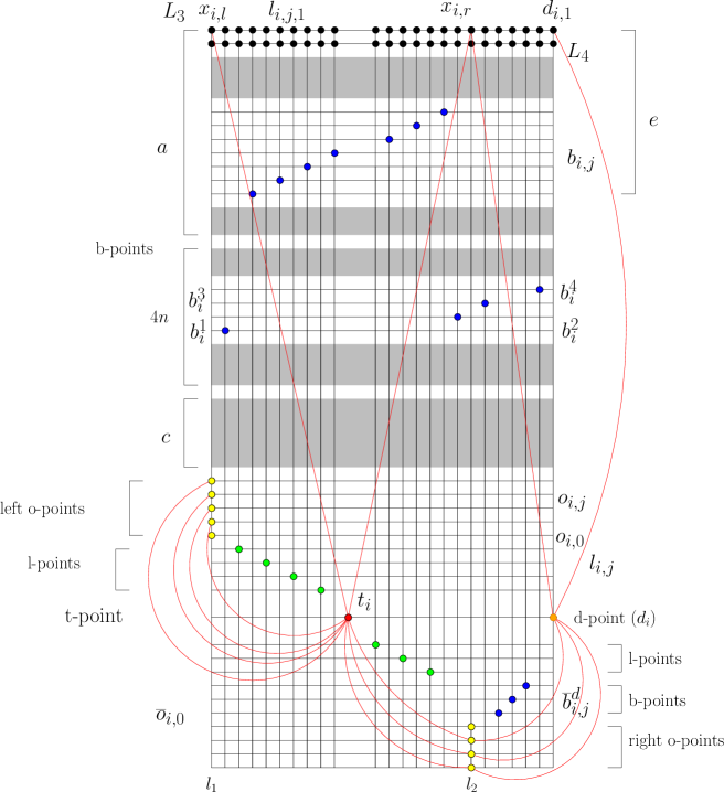
Figure 7: The variable pattern for $x_{i}$. The t-point, o-points, l-points, d-point and b-points are shown in the figure, along with the names of their corresponding vertices. The gray areas represent multiple horizontal lines. Some non-edges are drawn as curves. The lines $l_{1}$ and $l_{2}$ are the left and right o-lines of $x_{i}$ respectively.

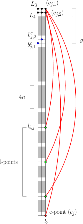
Figure 8: The clause pattern for $C_{j}$. The c-point, l-points and b-point are shown in the figure, along with the names of their corresponding vertices. The gray areas represent multiple horizontal lines. Non-edges are drawn as curves. The line $l_{3}$ is the c-line of $C_{j}$.

Based on the above classifications, we present the construction of $G^{\prime}(V^{\prime},E^{\prime})$. The sets of vertices associated with $x_{i}$ and $C_{j}$ are denoted as $V^{x}_{i}$ and $V^{c}_{j}$ respectively. Each $V^{x}_{i}$ contains the vertices $\{t_{i},d_{i},o_{i,0},\overline{o}_{{i},0},b^{1}_{i},b^{2}_{i},b^{3}_{i},b^{4}_{i}\}$. For every $C_{j}$ containing $x_{i}$ (or, $\overline{x_{i}}$), $V^{x}_{i}$ contains the vertices $\{o_{i,j},l_{i,j},b_{i,j}\}$ (respectively, $\{\overline{o}_{{i},j},\overline{l}_{{i},j},\overline{b}_{{i},j},\overline{b}^{d}_{{i},j}\}$). Each $V^{c}_{j}$ contains $c_{j}$, $b^{c}_{j,1}$, $b^{c}_{j,2}$, and $l_{{i},j}$ (or, $\overline{l}_{{i},j}$) corresponding to each $x_{i}$ (respectively, $\overline{x_{i}}$) in $C_{j}$. Hence,

$$V^{x}_{i} = \{t_{i},d_{i},o_{i,0},\overline{o}_{{i},0}\}\cup(\bigcup_{x_{i}\in C_{j}}\{o_{i,j},l_{i,j},b_{i,j}\})\cup(\bigcup_{\overline{x_{i}}\in C_{j}}\{\overline{o}_{{i},j},\overline{l}_{{i},j},\overline{b}_{{i},j},\overline{b}^{d}_{{i},j}\})\cup\{b^{1}_{i},b^{2}_{i},b^{3}_{i},b^{4}_{i}\}$$

$$V^{c}_{j} = \{c_{j}\}\cup(\bigcup_{x_{i}\in C_{j}}l_{{i},j})\cup(\bigcup_{\overline{x_{i}}\in C_{j}}\overline{l}_{{i},j})\cup\{b^{c}_{j,1},b^{c}_{j,2}\}$$

$$V^{\prime} = (\bigcup_{x_{i}\in\theta}V^{x}_{i})\cup(\bigcup_{C_{j}\in\theta}V^{c}_{j})$$

For every $x_{i},x_{k}\in\theta$, each vertex of $V^{x}_{i}$ is adjacent to every vertex of $V^{x}_{k}$. Similarly, for every $C_{j},C_{k}\in\theta$, each vertex of $V^{c}_{k}$ is adjacent to each vertex of $V^{c}_{k}$. The set of edges among vertices of $V^{x}_{i}$ (or, $V^{c}_{j}$) is denoted as $E^{x}_{i}$ (respectively, $E^{c}_{j}$). All vertices of $V^{x}_{i}$ are adjacent to each other except the o-vertices, and all left o-vertices are adjacent to all right o-vertices. The left o-vertices (or, right o-vertices) along with $t_{i}$ induce a path in $G^{\prime}$. The right o-vertices and $d_{i}$ induce a path in $G^{\prime}$ as well. All vertices of $E^{c}_{j}$ are adjacent to each other. For every $x_{i},C_{j}\in\theta$, each vertex of $V^{x}_{i}$ is adjacent to each vertex of $V^{c}_{j}$. Hence,

$$E^{x}_{i} = \Big{\{}(v_{a},v_{b})\mid v_{a}\neq v_{b}\ \textrm{and}\ v_{a},v_{b}\in V^{x}_{i}\setminus\Big{(}\{o_{i,0},\overline{o}_{{i},0}\}\cup(\bigcup_{x_{i}\in C_{j}}\{o_{i,j}\})\cup(\bigcup_{\overline{x_{i}}\in C_{j}}\{\overline{o}_{{i},j}\})\Big{)}\Big{\}}$$

$$\cup\Big{\{}(v_{a},v_{b})\mid v_{a}\in\{o_{{i},0}\}\cup(\bigcup_{x_{i}\in C_{j}}\{o_{i,j}\})\ \textrm{and}\ v_{b}\in\{\overline{o}_{{i},0}\}\cup(\bigcup_{\overline{x_{i}}\in C_{j}}\{\overline{o}_{{i},j}\})\Big{\}}$$

$$\cup\Big{\{}(v_{a},v_{b})\mid v_{a}\in\{o_{i,0},\overline{o}_{{i},0}\}\cup(\bigcup_{x_{i}\in C_{j}}\{o_{i,j}\})\cup(\bigcup_{\overline{x_{i}}\in C_{j}}\{\overline{o}_{{i},j}\})\ \textrm{and}$$

$$v_{b}\in V^{x}_{i}\setminus(\{t_{i},d_{i},o_{i,0},\overline{o}_{{i},0}\}\cup\Big{(}\bigcup_{x_{i}\in C_{j}}\{o_{i,j}\})\cup(\bigcup_{\overline{x_{i}}\in C_{j}}\{\overline{o}_{{i},j}\})\Big{)}\Big{\}}$$

$$\cup\Big{\{}(t_{i},o_{i,0}),(t_{i},\overline{o}_{{i},0}),(d_{i},\overline{o}_{{i},0})\Big{\}}\cup\Big{\{}(d_{i},v_{b})\mid v_{b}\in(\bigcup_{x_{i}\in C_{j}}\{o_{i,j}\})\Big{\}}$$

$$\cup\Big{\{}(o_{i,j},o_{i,k})\mid j<k\ \textrm{and}\ \nexists o_{i,l}\in V^{x}_{i}:i<l<k\Big{\}}$$

$$\cup\Big{\{}(\overline{o}_{i,j},\overline{o}_{i,k})\mid j<k\ \textrm{and}\ \nexists\overline{o}_{i,l}\in V^{x}_{i}:i<l<k\Big{\}}$$

$$E^{c}_{j} = \Big{\{}(v_{a},v_{b})\mid v_{a}\neq v_{b}\ \textrm{and}\ v_{a},v_{b}\in V^{c}_{j}\Big{\}}$$

$$E^{\prime} = \Big{\{}\bigcup_{x_{i}\in\theta}E^{x}_{i}\Big{\}}\cup\Big{\{}\bigcup_{C_{j}\in\theta}E^{c}_{j}\Big{\}}\cup\Big{(}\bigcup_{x_{i}\in\theta}\{(v_{a},v_{b})\mid v_{a}\in V^{x}_{i}\ \textrm{and}\ v_{b}\in V^{\prime}\setminus V^{x}_{i}\}\Big{)}$$

$$\cup\Big{(}\bigcup_{C_{j}\in\theta}\{(v_{a},v_{b})\mid v_{a}\in V^{c}_{j}\ \textrm{and}\ v_{b}\in V^{\prime}\setminus V^{c}_{j}\}\Big{)}$$

We have the following lemma on the size of $G^{\prime}$.

Lemma 7.

There are $(8n+12m+\sum\limits_{x_{i}\in\theta}\overline{n_{i}})$ vertices in $G^{\prime}$.

Proof.

We know from the construction of $G^{\prime}$ that the number of t-vertices is $n$, the number of d-vertices is $n$, the number of o-vertices is $(3m+2n)$, the number of l-vertices is $3m$, the number of c-vertices is $m$, and the number of b-vertices is $(4n+5m+\sum\limits_{x_{i}\in\theta}\overline{n_{i}})$ in $G$. So, $G^{\prime}$ has a total of $(8n+12m+\sum\limits_{x_{i}\in\theta}\overline{n_{i}})$ vertices. ∎

4.2 Construction of a reduction graph

Here, we construct the reduction graph $G^{\prime\prime}(V^{\prime\prime},E^{\prime\prime})$ such that $G^{\prime\prime}$ is a PVG if and only if $\theta$ is satisfied. From Lemma 7, we know that the number of vertices in $G^{\prime}$ is $(8n+12m+\sum\limits_{x_{i}\in\theta}\overline{n_{i}})$. To get $G^{\prime\prime}$ with certain restrictions on its possible visibility embeddings, we need to join $G^{\prime}$ to a modified slanted grid graph $G$ with edges such that $|G|\sim|G^{\prime}|^{8}$. Let $\alpha=12(m+n)$. Since $\alpha>(8n+12m+\sum\limits_{x_{i}\in\theta}\overline{n_{i}})$, but we do not actually require so many vertical lines to embed the 3-SAT graph, the modified slanted grid graph $G(V,E)$ is constructed starting from a $\alpha\times\alpha$ slanted grid graph, and $m_{0}=3m$, as stated in Section 3.1. The vertices of $G^{\prime\prime}$ are the vertices of $G$ and $G^{\prime}$. Hence, $V^{\prime\prime}=V\cup V^{\prime}$. Consider the unique visibility embedding of $G$, with $p_{1}$ and $p_{2}$ as the rightmost and topmost embedding points, respectively. The $i^{th}$ horizontal line from the top and the $i^{th}$ vertical line from the left are denoted by $l^{h}_{i}$ and $l^{v}_{i}$ respectively. The vertex of $V$ that corresponds to the embedding point at the intersection of the $i^{th}$ vertical and $j^{th}$ horizontal lines, is denoted by $v(l^{v}_{i},l^{h}_{j})$. Now we assign similar coordinates to vertices of $V^{\prime}$. Note that we may assign a set of possible coordinates to the same vertex, in order to facilitate the analysis of embeddings of $G^{\prime\prime}$. For each variable $x_{i}\in\theta$, coordinates are assigned to vertices of $V^{x}_{i}$ as follows (Figure 7).

1. Corresponding to each variable $x_{i}$, distinct horizontal lines are occupied by $n_{i}+\overline{n_{i}}+2$ o-points, $n_{i}+\overline{n_{i}}$ l-points and $n_{i}+2\overline{n_{i}}+4$ b-points. The points $t_{i}$ and $d_{i}$ occupy the same horizontal line. Hence, for all variables, a total of $9m+\sum\limits_{x_{i}\in\theta}\overline{n_{i}}+7n$ horizontal lines are occupied by embedding points. There are six points for each clause. However, the three l-points for each clause are already counted for their corresponding variables, and the c-points of all the clauses occupy the same horizontal line. So, for all the clauses, a total of $2m+1$ horizontal lines are occupied excluding those occupied by the l-points. Hence, a total of $9m+\sum\limits_{x_{i}\in\theta}\overline{n_{i}}+7n+2m+1$ $=11m+\sum\limits_{x_{i}\in\theta}\overline{n_{i}}+7n+1$ horizontal lines are occupied. Let $a$ be a constant which marks the coordinates of the lowest b-point among all $b_{i,j}$ for all $i$ and $j$. There are $3m$ number of b-points of the form $b_{i,j}$, and the b-points for the clauses, $2m$ in number, occupy higher horizontal coordinates. So, $a=\alpha-(11m+\sum\limits_{x_{i}\in\theta}\overline{n_{i}}+7n+1)+3m+2m=\alpha-6m-\sum\limits_{x_{i}\in\theta}\overline{n_{i}}-7n-1$. Let $b$ denote the number of vertical lines occupied by the embedding points for the first $i-1$ variables. The two large horizontal lines at the top of any visibility embedding of $G$ have $2(\alpha)^{4}+\alpha$ embedding points each, and they occupy the same number of vertical lines. So, before the main grid structure where points corresponding to $G^{\prime}$ begins, $2(\alpha)^{4}$ vertical lines are occupied. Also, the embedding points of each variable $x_{i}$ occupy $(2n_{k}+3\overline{n_{{k}}}+7)$ vertical lines. So, $b=2(\alpha)^{4}+\sum_{k=1}^{i-1}(2n_{k}+3\overline{n_{{k}}}+7)$. Let, $c$ denote the number of horizontal lines occupied by embedding points corresponding to the first $i-1$ variables. Hence, by the previous calculations, $c=\sum_{k=1}^{i-1}(2n_{k}+3\overline{n_{{k}}}+3)$. For the time being, intuitively consider a variable pattern for the $i^{th}$ variable to be the region bounded by $l^{v}_{b+1}$, $l^{v}_{b+2n_{i}+3\overline{n_{i}}+7}$, $L_{3}$ and $l^{h}_{a+4n+c+2n_{i}+2\overline{n_{i}}+3+\overline{n_{i}}}$, though we describe the details of the corresponding embedding only in the next section. Note that the y-coordinates of the lowermost horizontal lines of successive variable patterns give rise to a staircase-like structure as seen in Figure 9.

2. The t-point may lie only on one of the two o-lines, and its x-coordinates correspond to those of the two o-lines. Horizontally, it lies below the $n_{i}+1$ left o-points. So, assign coordinates $(l^{v}_{b+1},l^{h}_{a+4n+c+2n_{i}+2})$ and $(l^{v}_{b+2n_{i}+2\overline{n_{i}}+4},l^{h}_{a+4n+c+2n_{i}+2})$ to $t_{i}$.

3. The points $o_{i,0}$ and $\overline{o}_{i,0}$ are the bottommost and topmost embedding points of the left and right o-lines, respectively. So, assign coordinates $(l^{v}_{b+1},l^{h}_{a+4n+c+n_{i}+1})$ and $(l^{v}_{b+2n_{i}+4},l^{h}_{a+4n+c+2n_{i}+2\overline{n_{i}}+3})$ to $o_{i,0}$ and $\overline{o}_{i,0}$ respectively.

4. The left o-line occupies the leftmost vertical line of a variable pattern. Its o-points lie on the consecutive horizontal lines, beginning from immediately below the lowest horizontal line of the $(i-1)^{th}$ variable pattern. Recall that the left o-vertices of $x_{i}$ induce a path along with $t_{i}$ in $G^{\prime}$. Let $S=(o_{i,l},\ldots,o_{i,0},t_{i})$ be the sequence of vertices in the path. Note that $S$ has $n_{i}+2$ elements. So, for each $o_{i,j}\in S$, $j\neq 0$, assign the coordinates $(l^{v}_{b+1},l^{h}_{a+4n+c+k})$ to $o_{i,j}$, where $o_{i,j}$ is the $k^{th}$ element of $S$.

5. The right o-line occupies a vertical line after the left o-line, all $n_{i}+\overline{n}_{i}$ l-points of the variable pattern, one b-point for each of the l-points, plus two more b-points lie on one vertical line each. Its o-points lie on the consecutive horizontal lines, beginning from immediately below the horizontal line for for the lowest b-point of the variable pattern, described later. Similar to the left o-vertices, the right o-vertices of $x_{i}$ induce a path along with $t_{i}$ in $G^{\prime}$. Let $\overline{S}=(t_{i},\overline{o}_{i,0},\ldots,\overline{o}_{i,l})$ be the sequence of vertices in the path. Note that $S$ has $\overline{n_{i}}+2$ elements. So, for each $\overline{o}_{i,j}\in\overline{S}$, $j\neq 0$, assign the coordinates $(l^{v}_{b+2n_{i}+2\overline{n_{i}}+4},l^{h}_{a+4n+c+2n_{i}+2\overline{n_{i}}+3+k})$ to $\overline{o}_{i,j}$, where $\overline{o}_{i,j}$ is the $(k+2)^{th}$ element of $\overline{S}$.

6. The l-points corresponding to the left o-points, lie on horizontal lines starting from immediately below the left o-points. If they lie inside the variable pattern at all, then they lie on vertical lines starting from the third leftmost vertical line of the variable pattern, leaving a vertical line in between each consecutive l-points, for a corresponding b-point. To each l-vertex $l_{i,j}$, assign coordinates $(l^{v}_{b+1+2k},l^{h}_{a+4n+c+n_{i}+1+k})$, where $o_{i,j}$ is the $k^{th}$ element of $S$. The line $l^{v}_{b+1+2k}$ is called an associated-line of $l_{i,j}$.

7. The l-points corresponding to the right o-points, lie on horizontal lines starting from immediately below the t-point. If they lie inside the variable pattern at all, they lie on vertical lines starting from two vertical lines to the right of the vertical line containing the rightmost left l-point of the variable pattern, leaving a vertical line in between each consecutive l-points, for a corresponding b-point. So, to each l-vertex $\overline{l}_{i,j}$ assign coordinates $(l^{v}_{b+2n_{i}+1+2k},l^{h}_{a+4n+c+2n_{i}+2+k})$, where $\overline{o}_{i,j}$ is the $(k+2)^{th}$ element of $\overline{S}$. The line $l^{v}_{b+1+2k}$ is called an associated-line of $\overline{l}_{i,j}$.

8. The d-point $d_{i}$ lies in the same horizontal line as that of $t_{i}$, and either on the right o-line, or on the rightmost vertical line of the variable pattern. So, assign coordinates $(l^{v}_{b+2n_{i}+2\overline{n_{i}}+4},l^{h}_{a+4n+c+2n_{i}+2})$ and $(l^{v}_{b+2n_{i}+3\overline{n_{i}}+7},l^{h}_{a+4n+c+2n_{i}+2})$ to $d_{i}$.

9. Assign coordinates $(l^{v}_{b+2},l^{h}_{a+4(n-i)+4})$, $(l^{v}_{2(n_{i}+\overline{n_{i}})+3},l^{h}_{a+4(n-i)+3})$, $(l^{v}_{2(n_{i}+\overline{n_{i}})+5},l^{h}_{a+4(n-i)+2})$ and
   $(l^{v}_{2n_{i}+3\overline{n_{i}}+6},l^{h}_{a+4(n-i)+1})$ to the b-vertices $b^{1}_{i}$, $b^{2}_{i}$, $b^{3}_{i}$ and $b^{4}_{i}$ respectively.

10. Let $e=\alpha+n-(8n+12m+\sum\limits_{x_{i}\in\theta}\overline{n_{i}})+\sum_{p=i}^{n}(n_{p}+n_{\overline{p}})+5m-1$. The b-points of the forms $b_{i,j}$ and $\overline{b}_{i,j}$ lie on consecutive horizontal lines starting from $l^{h}_{e}$ in a bottom to top manner. Between each such b-point, there is a vertical line for accommodating an l-point. Assign coordinates $(l^{v}_{b+2+2k},l^{h}_{e+1-k})$ to $b_{i,j}$, where $o_{i,j}$ is the $k^{th}$ element of $S$. Similarly, assign coordinates $(l^{v}_{b+2n_{i}+2+2k},l^{h}_{e+\overline{n_{i}}+1-k})$ to $\overline{b}_{i,j}$, where $\overline{o}_{i,j}$ is the $(k+2)^{th}$ element of $\overline{S}$.

11. The lowest group of b-points of the variable pattern lie in between the right o-line and the rightmost vertical line of the variable pattern. Their function is to block $d_{i}$ from the right o-points when $d_{i}$ lies on the rightmost vertical line of the variable pattern. So, assign coordinates $\{(l^{v}_{2(n_{i}+\overline{n_{i}})+5+k},l^{h}_{a+4n+c+2n_{i}+2\overline{n_{i}}+3-k})$ to each $\overline{b}^{d}_{i,j}$, where $\overline{o}_{i,j}$ is the $(k+2)^{th}$ element of $\overline{S}$.

From the assignment of coordinates to the above vertices, for the time being, intuitively consider the $j^{th}$ clause pattern to be the region bounded by the lines $l^{v}_{f}$, $l^{v}_{f+3}$, $L_{3}$ and $l^{h}_{\alpha}$ though we describe the details of the corresponding embedding only in the next section. For each clause $C_{j}\in\theta$ , coordinates are assigned to the vertices of $V^{c}_{j}$ as follows (Figure 8).

1. Let $f$ denote the x-coordinate of the rightmost vertical line of the $(j-1)^{th}$ clause pattern. The rightmost vertical line of the $n^{th}$ variable pattern has x-coordinate $2(\alpha)^{4}(\sum_{k=1}^{n}(2n_{k}+3n_{\overline{k}}+7))$. The first $j-1$ clause patterns occupy $3(j-1)$ vertical lines. So, $f=2(\alpha)^{4}+(\sum_{k=1}^{n}(2n_{k}+3n_{\overline{k}}+7))+3(j-1)$. Let $g$ denote the y-coordinate of the lowest b-point in the $j^{th}$ clause pattern. There are a total $3m$ b-points of the form $b_{i,j}$ and $\overline{b}_{i,j}$ in all the variable patterns and these b-points are below the b-points of any clause pattern. There are two b-points occupying two distinct horizontal lines in each clause pattern. So, $g=a-3m-2(j-1)$.

2. The l-points remain in the horizontal lines already assigned to them. However, they may lie on the c-line to satisfy the clause or another vertical line of the clause pattern. Assign coordinates $(l^{v}_{f+3},l^{h}_{y})$ to $l_{i,j}$ (or, $\overline{l}_{i,j}$), where $l^{h}_{y}$ is the second component of coordinates assigned to $l_{i,j}$ (respectively, $\overline{l}_{i,j}$) earlier.

3. Assign coordinates $(l^{v}_{f+10},l^{h}_{g})$ and $(l^{v}_{f+11},l^{h}_{g-1})$ to $b^{c}_{j,1}$ and $b^{c}_{j,2}$ respectively. Whichever l-points of $C_{j}$ lie on there associated lines, are blocked by $b^{c}_{j,1}$ and $b^{c}_{j,2}$ from $c_{j,1}$.

4. The c-point of the clause pattern lies on the rightmost vertical line of the clause pattern and the bottommost horizontal line of the grid. So, assign coordinates $(l^{v}_{f+3},l^{h}_{\alpha})$ to $c_{i}$.

Before we define the edge set of $G^{\prime\prime}$, we need the following definitions related to coordinates assigned to the vertices of $V^{\prime\prime}$. For every vertex $q\in V^{\prime\prime}\setminus\{v_{1},v_{2}\}$, let $S^{q}$ be the set of all pairs of coordinates assigned to $q$. Furthermore, for every vertex $q\in V^{\prime\prime}\setminus\{v_{1},v_{2}\}$, let $S^{q}_{x}$ and $S^{q}_{y}$ be the sets of the first and second components, respectively, of all pairs of coordinates assigned to $v$. Consider vertices $v_{a}$ and $v_{b}$, such that $v_{a}\in V^{\prime}$ and $v_{b}\in V\setminus\{v_{1},v_{2}\}$. Suppose that there exists some $l^{v}_{x_{1}}\in S^{v_{a}}_{x}\cap S^{v_{b}}_{x}$ such that $(l^{v}_{x_{1}},l^{h}_{y_{1}})\in S^{v_{a}}$ and $(l^{v}_{x_{1}},l^{h}_{y_{2}})\in S^{v_{b}}$ for some $y_{1}$ and $y_{2}$. Then we refer to the pair $(v_{a},v_{b})$ as a vertical neighbouring pair if there is no $v_{c}$ with $v_{c}\neq v_{a}$ and $v_{c}\neq v_{b}$ and $(l^{v}_{x_{1}},l^{h}_{y_{3}})\in S^{v_{c}}$ such that $y_{1}>y_{3}>y_{2}$. Similarly, suppose that there exists some $l^{h}_{y_{1}}\in S^{v_{a}}_{y}\cap S^{v_{b}}_{y}$ such that $(l^{v}_{x_{1}},l^{h}_{y_{1}})\in S^{v_{a}}$ and $(l^{v}_{x_{2}},l^{h}_{y_{1}})\in S^{v_{b}}$ for some $x_{1}$ and $x_{2}$. Then we refer to the pair $(v_{a},v_{b})$ as a horizontal neighbouring pair if there is no $v_{c}$ with $v_{c}\neq v_{a}$ and $v_{c}\neq v_{b}$ and $(l^{v}_{x_{3}},l^{h}_{y_{1}})\in S^{v_{c}}$ such that $x_{1}<x_{3}<x_{2}$. Let $L(G^{\prime\prime})$ be the set of all such vertical or horizontal neighbouring pairs possible from the vertices of $V^{\prime\prime}\setminus\{v_{1},v_{2}\}$. So, we have,

$$E^{\prime\prime} = E\cup E^{\prime}\cup\{(v_{a},v_{b})\mid v_{a}\in V^{\prime}\ \textrm{and}\ v_{b}\in V\setminus\{v_{1},v_{2}\}\ \textrm{and}\$$

$$((S^{v_{a}}_{x}\cap S^{v_{b}}_{x})\cup(S^{v_{a}}_{y}\cap S^{v_{b}}_{y})=\phi\ \textrm{or}\ (v_{a},v_{b})\in L(G^{\prime\prime}))\}$$

Based on the construction of $G^{\prime\prime}$, we state the following lemma without proof.

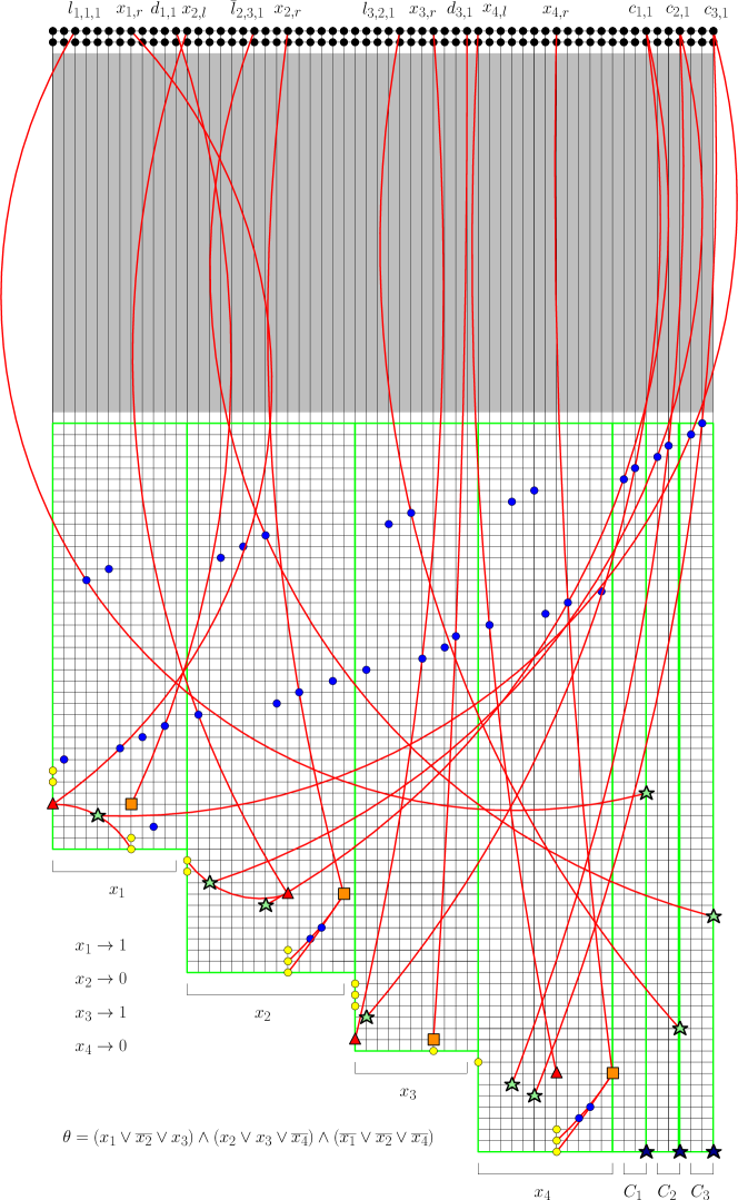
Figure 9: A canonical embedding $\psi$ of $G^{\prime\prime}$ corresponding to the given 3-SAT formula. The top two rows of embedding points are $L_{3}$ and $L_{4}$. The o-points, b-points, l-points, c-points, t-points and d-points are depicted as pale circles, dark circles, pale stars, dark stars, triangles and squares respectively. The non-horizontal and non-vertical line segments constitute $S_{L}$. Some non-edges corresponding to a visibility embedding, drawn here as red curves along with their blockers are as follows: $(t_{1},x_{1,r})\rightarrow b_{1}^{2}$, $(t_{1},\overline{o}_{1,3})\rightarrow\overline{l}_{1,3}$, $(d_{1},d_{1,1})\rightarrow b_{1}^{4}$, $(\overline{l}_{1,3},c_{3,1})\rightarrow b^{c}_{3,1}$, $(t_{2},x_{2,l})\rightarrow b_{2}^{1}$, $(t_{2},o_{2,2})\rightarrow l_{2,2}$, $(d_{2},x_{2,r})\rightarrow b_{2}^{3}$, $(d_{2},\overline{o}_{2,1})\rightarrow b^{d}_{2,1}$, $(d_{2},\overline{o}_{2,3})\rightarrow b^{d}_{2,3}$, $(l_{2,2},c_{2,1})\rightarrow b^{c}_{2,1}$, $(\overline{l}_{2,1},c_{1,1})\rightarrow b^{c}_{1,1}$, $(t_{3},x_{3,r})\rightarrow b_{3}^{2}$, $(d_{3},d_{3,1})\rightarrow b_{3}^{4}$, $(l_{3,1},c_{1,1})\rightarrow b^{c}_{1,2}$, $(t_{4},x_{4,l})\rightarrow b_{4}^{1}$, $(d_{4},x_{4,r})\rightarrow b_{4}^{3}$, $(d_{4},\overline{o}_{4,2})\rightarrow b^{d}_{4,2}$, $(d_{4},\overline{o}_{4,3})\rightarrow b^{d}_{4,3}$, $(\overline{l}_{4,2},c_{2,1})\rightarrow b^{c}_{2,2}$, $(\overline{l}_{4,3},c_{3,1})\rightarrow b^{c}_{3,2}$, $(l_{1,1},l_{1,1,1})\rightarrow b_{1,1}$, $(l_{3,2},l_{3,2,1})\rightarrow b_{3,2}$, $(\overline{l}_{2,3},\overline{l}_{2,3,1})\rightarrow\overline{b}_{2,3}$.

Lemma 8.

Given a 3-SAT formula $\theta$, the corresponding reduction graph $G^{\prime\prime}$ can be constructed in time polynomial in the size of $\theta$.

4.3 Canonical embeddings of reduction graphs

As stated earlier, we have shown the construction of the reduction graph $G^{\prime\prime}$ of $\theta$ in polynomial time. We study here some properties of $G^{\prime\prime}$. We need some definitions before we study these properties. An embedding $\psi$ of $G^{\prime\prime}$ is called a canonical embedding of $G^{\prime\prime}$ if (a) the embedding points of $\psi$ restricted to the vertices of $G$, form the unique visibility embedding of $G$, and (b) for all $v_{q}\in G^{\prime}$, the embedding point of $v_{q}$ is embedded on the intersection of horizontal and vertical lines giving a pair of coordinates that has been assigned to $v_{q}$. Observe that in a canonical embedding, the following hold true.

1. Each b-point is embedded only on its corresponding b-line.

2. Each c-point is embedded only on its corresponding c-line.

3. Each t-point is embedded only on one of its two o-lines.

4. Each d-point is embedded only on either its d-line or its right o-line.

5. Each o-point is embedded only on its o-line.

6. Each l-point is embedded either on its associated-line or its c-line.

If a canonical embedding $\psi$ of $G^{\prime\prime}$ is also a visibility embedding of $G^{\prime\prime}$, then $\psi$ is called a canonical visibility embedding of $G^{\prime\prime}$. We have the following lemma.

Lemma 9.

If $G^{\prime\prime}$ is a PVG then every visibility embedding of $G^{\prime\prime}$ is a canonical visibility embedding.

Proof.

We know from Lemmas 5 and 6 that $G$ has a unique visibility embedding. Let $\xi$ be the unique visibility embedding of $G$. Consider lines $L_{1}$, $L_{2}$, $L_{3}$ and $L_{4}$ in $\xi$ as before (Figure 3). Note that $|L_{3}|=|L_{4}|=2(\alpha)^{4}$ Let $G^{\prime\prime}$ be a PVG and $\xi^{\prime}$ be a visibility embedding of $G^{\prime\prime}$. Observe that the total number of embedding points in $\xi^{\prime}\setminus(L_{1}\cup L_{2}\cup L_{2}\cup L_{4})$ is less than $\alpha$. Moreover, the embedding points corresponding to the vertices of $G^{\prime}$ are visible from most embedding points of $L_{1}$, $L_{2}$, $L_{3}$ and $L_{4}$. So, $G^{\prime\prime}$ satisfies the conditions of Lemmas 5 and 6, and by a similar argument, it can be shown that the embedding points of $\xi^{\prime}$ restricted to the vertices of $G$, form the unique visibility embedding of $G$. Now we show that every vertex $v_{q}\in G^{\prime}$ satisfies the second condition of a canonical embedding. Consider the embedding point $l^{v}_{i}\cap L_{3}$ in $\xi^{\prime}$. Its corresponding vertex, by the construction of $G^{\prime\prime}$, is not adjacent to $v_{q}$ if and only if $l^{v}_{i}$ is assigned as a coordinate to $v_{q}$. A similar argument follows for $v_{q}$ and embedding points of the form $l^{h}_{j}\cap L_{1}$ in $\xi^{\prime}$. On the other hand, two non-consecutive embedding points on a horizontal or vertical line cannot be visible from each other. So, the embedding point of $v_{q}$ is embedded on the intersection of horizontal and vertical lines giving a pair of coordinates that has been assigned to $v_{q}$. Hence, $\xi^{\prime}$ is a canonical visibility embedding of $G^{\prime\prime}$. ∎

Let us define the variable pattern of each $x_{i}$ and the clause pattern of each $C_{j}$. For each $x_{i}$, let $a=\alpha-7n-6m-\sum\limits_{x_{i}\in\theta}\overline{n_{i}})-1$, $b=2(\alpha)^{4}+\sum_{k=1}^{i-1}(2n_{k}+3\overline{n_{{k}}}+7)$, and $c=\sum_{k=1}^{i-1}(2n_{k}+3\overline{n_{{k}}}+3)$, as defined in Section 4.2. For a canonical embedding $\xi$ of $G^{\prime\prime}$, the closed region bounded by the four lines $l^{v}_{b+1}$, $l^{v}_{b+2n_{i}+3\overline{n_{i}}+7}$, $L_{3}$ and $l^{h}_{a+4n+c+2n_{i}+2\overline{n_{i}}+3+\overline{n_{i}}}$ is called the variable pattern of $x_{i}$ (Figure 7). Let, for each $C_{j}$, let $f=2(\alpha)^{4}+(\sum_{k=1}^{n}(2n_{k}+3n_{\overline{k}}+7))+12(j-1)$, as defined in Section 4.2. For a canonical embedding $\xi$ of $G^{\prime\prime}$, the closed region bounded by the four lines $l^{v}_{f}$, $l^{v}_{f+12}$, $L_{3}$ and $l^{h}_{\alpha}$ is called the clause pattern of $C_{j}$ (Figure 8).

Lemma 10.

If $\theta$ is not satisfiable, then $G^{\prime\prime}$ does not have a canonical visibility embedding.

Proof.

Assume on the contrary that $\theta$ is not satisfiable but $G^{\prime\prime}$ has a canonical visibility embedding $\xi^{\prime}$. So, each t-point of $\xi^{\prime}$ is embedded on either its left o-line or right o-line. So, the embedding of the t-points corresponds to an assignment of the variables of $\theta$. Since one of the clauses (say, $C_{j}$) is not satisfied, the complements of the literals in $C_{j}$ have been assigned to $1$. Hence, if $l_{i,j}\in V^{c}_{j}$ then $t_{i}$ lies on the left o-line of $x_{i}$ and $l_{i,j}$ must be embedded in the variable pattern of $x_{i}$ in $\xi^{\prime}$. A similar argument holds if $\overline{l}_{i,j}$ is in $V^{c}_{j}$. This is true for all three literals of $C_{j}$. Hence, no l-point can be embedded in the clause pattern of $C_{j}$ in $\xi^{\prime}$. Therefore, there is no embedding point to block the visibility of the c-point from $c_{j,2}$, contradicting the assumption. ∎

Lemma 11.

If $\theta$ is not satisfiable, then $G^{\prime\prime}$ is not a PVG.

Proof.

The proof follows from Lemmas 9 and 10. ∎

4.4 Reduction from 3-SAT

In this Section we prove that if $\theta$ is satisfiable then $G^{\prime\prime}$ is a PVG. Recall that if $\theta$ is not satisfiable then $G^{\prime\prime}$ is not a PVG. We start by constructing a canonical embedding $\psi$ of $G^{\prime\prime}$, and then transform it into a canonical visibility embedding of $G^{\prime\prime}$. Let $S_{\theta}$ be a satisfying assignment of $\theta$. Since $G^{\prime\prime}=G\cup G^{\prime}$, all the embedding points corresponding to the vertices of $G$ are embedded initially to form the unique visibility embedding of $G$. Then, embedding points corresponding to $G^{\prime}$ are embedded to complete the embedding $\psi$ of $G^{\prime\prime}$ (Figure 9) as follows. Repeat the following three steps for all $x_{i}\in\theta$.

1. If $x_{i}$ is assigned $1$ in $S_{\theta}$ then embed the t-point of $t_{i}$ on its left o-line. Otherwise embed the t-point of $t_{i}$ on its right o-line.

2. If the t-point of $t_{i}$ is embedded on the its left o-line, then embed the d-point of $d_{i}$ on its right o-line. Otherwise embed the d-point of $d_{i}$ on its d-line.

3. If the t-point of $t_{i}$ is embedded on its left o-line, then embed the l-points of $l_{i,j}$ on their associated-lines, for all $j$. Otherwise embed the l-points of $\overline{l}_{i,j}$ on their associated-lines, for all $j$.

As a next step, for each clause $C_{j}$, choose an l-point of $C_{j}$ that has not been embedded yet, and embed it on the intersection of the c-line and a horizontal line corresponding to a pair of coordinates assigned to its c-vertex. Observe that such l-points are always available for each clause, since $S_{\theta}$ is a satisfying assignment of $\theta$. All the remaining l-points are embedded on their associated-lines. The construction of $\psi$ is completed by the following step.

1. Embed all the c-points and b-points on the intersection points representing the unique pair of coordinates assigned to them.

Before the above embedding $\psi$ is transformed to a visibility embedding $\xi$ of $G^{\prime\prime}$, we need the following lemma for rotating a line in $\psi$.

Lemma 12.

Consider a line $l^{\prime}$ of $\psi$. Let $\{p_{1},p_{2},\ldots,p_{q}\}$ denote the order of all embedding points on $l^{\prime}$ where $p_{i}$ lies on the intersection point of $l^{\prime}$ and a non-ordinary line $l_{i}$ (Figure 10(a)). For any given real $\epsilon>0$ and embedding point $p_{j}$ for $1\leq j\leq q$, $l^{\prime}$ can be rotated with $p_{j}$ as the pivot to form a new $l^{\prime}$ satisfying the following properties.

1. The embedding points of $\psi$ on $l^{\prime}$, except $p_{j}$, are relocated on the new $l^{\prime}$. All other embedding points in $\psi$ remain unchanged.

2. The order of embedding points on $l^{\prime}$ and the new $l^{\prime}$ are the same.

3. The order of embedding points on each $l_{i}$ also remains the same.

4. $\forall i\neq j,1\leq i\leq q$, $p_{i}$ does not lie on any other non-ordinary line.

5. For each $p_{i}$ on $l^{\prime}$, the Euclidean distance between the new and old positions of $p_{i}$ is less than $\epsilon$.

Proof.

Rotate $l^{\prime}$ with $p_{j}$ as the pivot in clockwise direction until it reaches a point $y$ on some line $l_{i}$ such that $y$ is either an intersection point of $\psi$ or the length of the segment $p_{i}y$ is $\epsilon$. The new $l^{\prime}$ is the line through $p_{j}$ and some point in the interior of $p_{i}y$. Embed each $p_{i}$ on the intersection point of $l_{i}$ and the new $l^{\prime}$ (Figure 10(b)). It can be seen that the properties (a), (c), (b), (d) and (e) of the lemma are satisfied. ∎

Observe that in $\psi$, there can be several non-ordinary lines that are not horizontal or vertical lines. The blocking relationships induced by these lines may not conform to the edges in $G^{\prime}$. Treating each vertical line as $l^{\prime}$ and each horizontal line intersecting $l^{\prime}$ as $l_{i}$, Lemma 12 is applied on every vertical line in $\psi$ by rotating around $p_{2}$. Thus, any non-ordinary line that now passes through an embedding point of $\psi$ is either a vertical or a horizontal line. We have the following lemma on rotating multiple lines of $\psi$.

Figure 10: (a) The lines $l_{1},l_{2},l_{3},l_{4}$ and $l_{5}$ intersect $l^{\prime}$ at $p_{1}$, $p_{2}$, $p_{3}$, $p_{4}$ and $p_{5}$ respectively. (b) The line $l^{\prime}$ is rotated around $p_{2}$, so that all embedding points on $l^{\prime}$ except $v_{2}$ are relocated. Each of the relocated embedding points lie on exactly two non-ordinary lines and within $\epsilon$ distance of their previous positions.

Lemma 13.

Consider a vertical line $l^{\prime}$ of $\psi$. Let $(w_{i},w_{i+1},\ldots,w_{i+j-1},w_{i+j})$ be all embedding points on $l^{\prime}$ from $w_{i}$ to $w_{i+j}$ such that they lie on the intersection points of $l^{\prime}$ with $(l_{i},l_{i+1},\ldots,l_{i+j-1},l_{i+j})$ respectively. Let $q_{1}$ and $q_{2}$ be any two designated points on the interval $w_{i+1}w_{i+j-1}$. For every line $l_{i+k}\in(l_{i+1},\ldots,l_{i+j-1})$, a new $l_{i+k}$ can be constructed such that $l_{i+k}$ intersects $l^{\prime}$ at a point $r_{k}$ satisfying the following properties.

1. The points $(r_{1},r_{2},\ldots,r_{j-1})$ lie on $q_{1}q_{2}$ and their order follows the order of $(w_{i},w_{i+1},\ldots,w_{i+j-1},w_{i+j})$.

2. The non-ordinary lines passing through the embedding points on $(l_{i},l_{i+1},\ldots,l_{i+j-1},l_{i+j})$ are either vertical or horizontal lines.

Proof.

Let $p^{\prime}_{1}$ be a point on $q_{1}q_{2}$. Set $\epsilon=\frac{1}{2}\min(q_{1}r^{\prime}_{1},r^{\prime}_{1}q_{2})$ Rotate the line passing through $r^{\prime}_{1}$ and $p_{1}$ with $p_{1}$ as the pivot using Lemma 12 to obtain a new intersection point $r_{1}$ on $l^{\prime}$. The line passing through $p_{1}$ and $r_{1}$ is the new $l_{1}$, and embedding points on $l_{1}$ are relocated on the corresponding intersection points of the new $l_{1}$. Analogously, choose a point $r^{\prime}_{2}$ on $r_{1}q_{2}$ and construct the new $l_{2}$ giving a new intersection point $r_{2}$ of $l^{\prime}$ on $r_{1}q_{2}$. These operations are performed on all lines in $(l_{i+1},\ldots,l_{i+j-1})$. It can be seen that the properties (a) and (b) of the lemma are satisfied. ∎

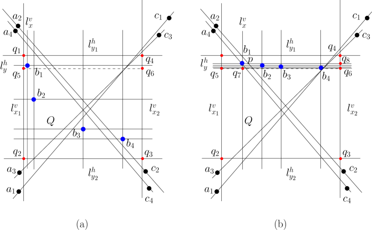
Figure 11: (a) The embedding points $b_{1}$, $b_{2}$, $b_{3}$ and $b_{4}$ of $B$ lie in the interior of the quadrilateral $q_{1}q_{2}q_{3}q_{4}$. (b) The embedding points $b_{1}$, $b_{2}$, $b_{3}$ and $b_{4}$ of $B$ are relocated inside $q_{1}q_{5}q_{6}q_{4}$, with $b_{1}$ blocking the segment $a_{4}c_{4}$.

Using Lemma 13, we show that embedding points inside a special type of quadrilateral can be relocated as blockers of pairs of embedding points lying outside the quadrilateral. Consider a quadrilateral $Q=(q_{1},q_{2},q_{3},q_{4})$, where $q_{1}$, $q_{2}$, $q_{3}$ and $q_{4}$ are embedding points of $\psi$ lying on $(l^{v}_{x_{1}},l^{h}_{y_{1}})$, $(l^{v}_{x_{1}},l^{h}_{y_{2}})$, $(l^{v}_{x_{2}},l^{h}_{y_{2}})$ and $(l^{v}_{x_{2}},l^{h}_{y_{1}})$ respectively, and $x_{1}<x_{2}$ and $y_{1}<y_{2}$. Let $B$ be the set of all embedding points lying inside $Q$. $B$ is said to be an ordered set if no two embedding points of $B$ lie on the same horizontal or vertical line, and $B$ satisfies exactly one of the following properties.

1. For all embedding points $b^{\prime}\in B$ and $b^{\prime\prime}\in B$ embedded on $(l^{v}_{x^{\prime}},l^{h}_{y^{\prime}})$ and $(l^{v}_{x^{\prime\prime}},l^{h}_{y^{\prime\prime}})$ respectively, if $x^{\prime}<x^{\prime\prime}$ (or, $x^{\prime}>x^{\prime\prime}$) then $y^{\prime}<y^{\prime\prime}$ (respectively, $y^{\prime}>y^{\prime\prime}$).

2. For all embedding points $b^{\prime}\in B$ and $b^{\prime\prime}\in B$ embedded on $(l^{v}_{x^{\prime}},l^{h}_{y^{\prime}})$ and $(l^{v}_{x^{\prime\prime}},l^{h}_{y^{\prime\prime}})$ respectively, if $x^{\prime}<x^{\prime\prime}$ (or, $x^{\prime}>x^{\prime\prime}$) then $y^{\prime}>y^{\prime\prime}$ (respectively, $y^{\prime}<y^{\prime\prime}$).

Let $A$ be a set of embedding points of $\psi$ such that each $a_{i}\in A$ lies to the left of $l^{v}_{x_{1}}$ and also lies either above $l^{h}_{y_{1}}$ or below $l^{h}_{y_{2}}$. Let $C$ be a set of embedding points of $\psi$ such that each $c_{i}\in C$ lies to the right of $l^{v}_{x_{2}}$ and also lies either above $l^{h}_{y_{1}}$ or below $l^{h}_{y_{2}}$. Let $S$ be a set of line segments $a_{i}c_{j}$ where $a_{i}\in A$ and $c_{j}\in C$, and $a_{i}c_{j}$ intersects both $q_{1}q_{4}$ and $q_{2}q_{3}$. A pentuple $U=(Q,A,B,C,S)$ is called a good pentuple if $|B|\geq|S|$, and $B$ is an ordered set.

Lemma 14.

For a given good pentuple $U=(Q,A,B,C,S)$ in $\psi$, horizontal and vertical lines passing through the embedding points of $B$ can be relocated satisfying the following properties.

1. All horizontal and vertical lines in $\psi$ retain their angular ordering around $p_{1}$ and $p_{2}$ respectively.

2. Each embedding point in $B$ lies on exactly one segment of $S$.

3. Each embedding point in $B$ lies on exactly three non-ordinary lines, two of which are horizontal and vertical lines.

4. For every horizontal or vertical line $l^{\prime\prime}$ containing $b\in B$, no embedding point on $l^{\prime\prime}\setminus\{b\}$ lies on a third non-ordinary line after relocation.

Proof.

Wlog let $B$ satisfy Property $1$ of ordered sets. Choose an appropriate point $q_{5}\in q_{1}q_{2}$ such that no intersecting points of the segments of $S$ lie in the interior of $q_{1}q_{5}q_{6}q_{4}$, where $q_{6}$ is the point of intersection of $p_{1}q_{5}$ and $q_{3}q_{4}$ (Figure 11(a)). Let $H_{Q}$ and $V_{Q}$ be the set of all horizontal and vertical lines passing through $Q$, respectively. By applying Lemma 13 on any vertical line in $V_{Q}$, relocate all horizontal lines of $H_{Q}$ such that all of them pass through $q_{1}q_{5}q_{6}q_{4}$. Observe that all embedding points of $B$ have moved inside $q_{1}q_{5}q_{6}q_{4}$. Since none of the segments of $S$ intersect inside $q_{1}q_{5}q_{6}q_{4}$, they have a left to right order defined by their intercepts on $q_{5}q_{6}$. Let $a_{i}c_{j}$ be the leftmost segment of $S$ in this order. Denote the leftmost embedding point of $B$ as $b$, and let $l^{v}_{x}$ and $l^{h}_{y}$ be its vertical and horizontal lines respectively. Applying Lemma 13 on any horizontal line in $H_{Q}$, all vertical lines of $V_{Q}$ are relocated such that $l^{v}_{x}$ intersects $a_{i}c_{j}$ at a point (say, $p$) (Figure 11(b)), maintaining other lines of $V_{Q}$ passing through $q_{1}q_{5}q_{6}q_{4}$. Treating $p$ as an embedding point and taking $p_{2}$ as the pivot, Lemma 12 can be applied on $l^{v}_{x}$ to ensure that $p$ does not lie on any other non-ordinary line. Now embed $b$ on $p$ by relocating $l^{h}_{y}$ accordingly. Relocate all other horizontal lines of $H_{Q}$ by applying Lemma 13, maintaining all lines of $H_{Q}$ passing through $q_{1}q_{5}q_{6}q_{4}$. It can be seen that $U^{\prime}=(bq_{7}q_{3}q_{8},A,B\setminus\{b\},C,S\setminus\{a_{i}c_{j}\})$ is a good pentuple, where $q_{7}=l^{v}_{x}\cap q_{5}q_{6}$ and $q_{8}=l^{h}_{y}\cap q_{3}q_{4}$. Repeating the above procedure, embedding points of $B$ are placed on all segments of $S$ as blockers, satisfying properties (a), (b), (c) and (d) of the lemma. Analogous arguments of the proof are applicable if $B$ satisfies Property $2$ of ordered sets. ∎

Now we use Lemmas 12, 13 and 14 to finally transform $\psi$ into a visibility embedding $\xi$ of $G^{\prime\prime}$. We have the following lemma.

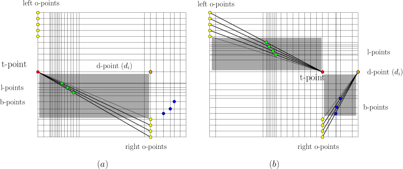
Figure 12: (a) Since t-point lies on the left o-line, blockers are placed between t-point and right o-points. The quadrilateral required for a good pentuple is shaded in gray. (b) Since t-point lies on the right o-line, blockers are placed between t-point and left o-points. Since b-point lies on the d-line, blockers are placed between d-point and right o-points. Quadrilaterals required for a good pentuple are shaded in gray.

Lemma 15.

The canonical embedding $\psi$ can be transformed into a visibility embedding $\xi$ of $G^{\prime\prime}$.

Proof.

The only adjacency relationships of $G^{\prime\prime}$ that $\psi$ may not satisfy are those $(i)$ between o-vertices and t-vertices, $(ii)$ between o-vertices and d-vertices, and $(iii)$ between t-vertices, l-vertices, d-vertices and vertices corresponding to certain points on $L_{3}$. Consider $(i)$ and $(ii)$. For each $x_{i}$, if the t-point of $t_{i}$ is embedded on its left o-line, then consider the quadrilateral $Q$ formed by the horizontal line passing through the topmost right o-point, horizontal line of the t-point, left o-line and right o-line. Draw two more vertical and horizontal lines such that they form a quadrilateral $Q^{\prime}$ in the interior of $Q$, and only nominally smaller than $Q$. It can be seen that $Q^{\prime}$, $t_{i}$, the right o-points, the l-points of the form $\overline{l}_{i,j}$, and all segments between the t-point and the right o-points form a good pentuple. Hence these segments can be blocked by relocating the corresponding l-points using Lemma 14 (Figure 12 (a)). A similar argument works if the t-point is embedded on the right o-line (Figure 12 (b)), or if the d-point is embedded on the d-line (Figure 12 (b)). Consider $(iii)$. Let $S_{L}$ be all such segments having an endpoint on $L_{3}$ (Figure 9). Locate a point $p_{3}$ on $l^{h}_{1}$ such that $L_{3}$ and $L_{4}$ are above and below $p_{1}p_{3}$ respectively. Moreover, the intersection points of $S_{L}$ with vertical lines of $\psi\setminus\{L_{3}\}$ lie below $p_{1}p_{3}$. Let $H_{L}$ be the set of all horizontal lines between $L_{3}$ and $l^{h}_{a+4n+1}$, where $a=\alpha-7n-6m\sum\limits_{x_{i}\in\theta}\overline{n_{i}}-1$ as stated in Section 4.2. Apply lemma 13 on any vertical line of $\psi$, and treating its intersection points with horizontal lines as embedding points, all horizontal lines of $H_{L}$ are relocated so that they are above ${p_{1}p_{3}}$. Consider any segment $s_{j}\in S_{L}$. Let the two endpoints of $s_{j}$ in $\psi$ be $r_{1}(s_{j})$ and $r_{2}(s_{j})$, where $r_{1}(s_{j})\in L_{3}$. Let the two vertical lines passing through $r_{1}(s_{j})$ and $r_{2}(s_{j})$ be $l^{v}_{u_{j}}$ and $l^{v}_{w_{j}}$ respectively. Observe that if $u_{j}<w_{j}$ (or, $u_{j}>w_{j}$) then $l^{v}_{u_{j}+1}$ (respectively, $l^{v}_{u_{j}-1}$) contains a b-point lying on a horizontal line of $H_{L}$, due to the construction of $\psi$. Such a b-point exists for every segment in $S_{L}$. For two segments of $S_{L}$ with a common endpoint on a c-line, the two b-points on the two vertical lines immediately to the left of the c-line correspond to the two segments. Let $B_{L}$ denote the set of all these b-points. Now consider a b-point $b_{i}\in B_{L}$ such that the horizontal line passing through $b_{i}$ (say, $l^{h}_{y_{i}}$) is lower than the horizontal line passing through any other b-point of $B_{L}$. Let $s_{i}\in S_{L}$ be the segment corresponding to $b_{i}$. Let $Q_{i}$ be the quadrilateral enclosed by $l^{v}_{u_{i}}$, $l^{v}_{u_{i+2}}$, ${p_{1}p_{3}}$ and $l^{h}_{y_{i}-1}$, assuming $u_{i}<w_{i}$. Observe that $Q_{i}$, $B_{i}=\{b_{i}\}$, $A_{i}=\{r_{1}(s_{i})\}$, $C_{i}=\{r_{2}(s_{i})\}$ and $S_{i}=\{s_{i}\}$ constitute a good pentuple, say, $U_{i}$. Apply Lemma 14 on $U_{i}$ to place $b_{i}$ as a blocker on $s_{i}$. Remove $b_{i}$ and $s_{i}$ from $B_{L}$ and $S_{L}$ respectively. Remove $l^{h}_{y_{i}}$ and all horizontal lines below it from $H_{L}$. Repeat the process on the lowest b-point of $B_{L}$, treating $l^{h}_{y_{i}}$ as the new $p_{1}p_{3}$. It may so happen that the same embedding point on $L_{3}$ is the endpoint of two segments $s_{i}$ and $s_{j}$ in $S_{L}$, i.e., $r_{1}(s_{i})=r_{1}(s_{j})$. This case arises only when $r_{1}(s_{i})$ and $r_{1}(s_{j})$ lie on a c-line of $\psi$. In this case, the two b-points on the two vertical lines immediately to the left of the c-line are relocated as blockers on $s_{i}$ and $s_{j}$, using an analogous process. Hence, b-points can be assigned as blockers on segments of $S_{L}$ in cases $(i)$, $(ii)$ and $(iii)$. Therefore, the canonical embedding $\psi$ can be transformed into a visibility embedding $\xi$ of $G^{\prime\prime}$. ∎

Finally, we have the following theorem.

Theorem 1.

The recognition problem for PVGs in NP-hard.

Proof.

Given a 3-SAT formula $\theta$, the construction of the corresponding graph $G^{\prime\prime}$ takes polynomial time, due to Lemma 8. The graph $G^{\prime\prime}$ is a PVG if and only if $\theta$ is satisfiable, due to Lemma 11 and Lemma 15. Hence the recognition problem for PVGs in NP-hard. ∎

Corollary 1.

The reconstruction problem for PVGs in NP-hard.

5 Concluding remarks

In this paper we have proved that the recognition and reconstruction problems for point visibility graphs, are NP-hard. On the other hand, we know that the recognition problem for point visibility graphs is in PSPACE [7]. It has been pointed out by Ghosh and Goswami [6] that the recognition problem for point visibility graphs, and to show whether the problem lies in NP, are still open.

6 Acknowledgements

The author would like to thank Jean-Lou De Carufel, Anil Maheshwari and Michiel Smid for the many discussions that helped to structure the paper. The author would also like to thank Amitava Bhattacharya, and Prahladh Harsha for their valuable suggestions. The author is specially thankful to the anonymous referees and Subir Kumar Ghosh for their suggestions which have improved the presentation of the paper significantly.

References

- [1] B. Chazelle, L. J. Guibas, and D.T. Lee. The power of geometric duality. BIT, 25:76–90, 1985.
- [2] M. de Berg, O. Cheong, M. Kreveld, and M. Overmars. Computational Geometry, Algorithms and Applications. Springer-Verlag, 3rd edition, 2008.
- [3] R. Diestel. Graph Theory. Springer-Verlag, 2005.
- [4] H. Edelsbrunner, J. O’Rourke, and R. Seidel. Constructing arrangements of lines and hyperplanes with applications. SIAM Journal on Computing, 15:341–363, 1986.
- [5] S. K. Ghosh. Visibility Algorithms in the Plane. Cambridge University Press, 2007.
- [6] S. K. Ghosh and P. P. Goswami. Unsolved problems in visibility graphs of points, segments and polygons. ACM Computing Surveys, 46(2):22:1–22:29, December, 2013.
- [7] S. K. Ghosh and B. Roy. Some results on point visibility graphs. In Proceedings of the Eighth International Workshop on Algorithms and Computation, volume 8344 of Lecture Notes in Computer Science, pages 163–175. Springer-Verlag, 2014.
- [8] J. Kára, A. Pór, and D. R. Wood. On the Chromatic Number of the Visibility Graph of a Set of Points in the Plane. Discrete & Computational Geometry, 34(3):497–506, 2005.
- [9] T. Lozano-Perez and M. A. Wesley. An algorithm for planning collision-free paths among polyhedral obstacles. Communications of ACM, 22:560–570, 1979.
- [10] M. S. Payne, A. Pór, P. Valtr, and D. R. Wood. On the connectivity of visibility graphs. Discrete & Computational Geometry, 48(3):669–681, 2012.
- [11] F. Pfender. Visibility graphs of point sets in the plane. Discrete & Computational Geometry, 39(1):455–459, 2008.
- [12] L.G. Shapiro and R.M. Haralick. Decomposition of two-dimensional shape by graph-theoretic clustering. IEEE Transactions on Pattern Analysis and Machine Intelligence, PAMI-1:10–19, 1979.