On the Permanence of Vertices in Network Communities

Abstract

Despite the prevalence of community detection algorithms, relatively less work has been done on understanding whether a network is indeed modular and how resilient the community structure is under perturbations. To address this issue, we propose a new vertex-based metric called permanence, that can quantitatively give an estimate of the community-like structure of the network.

The central idea of permanence is based on the observation that the strength of membership of a vertex to a community depends upon the following two factors: (i) the distribution of external connectivity of the vertex to individual communities and not the total external connectivity, and (ii) the strength of its internal connectivity and not just the total internal edges.

In this paper, we demonstrate that compared to other metrics, permanence provides (i) a more accurate estimate of a derived community structure to the ground-truth community and (ii) is more sensitive to perturbations in the network. As a by-product of this study, we have also developed a community detection algorithm based on maximizing permanence. For a modular network structure, the results of our algorithm match well with ground-truth communities.

1 Introduction

Finding accurate community structures, i.e., groups of vertices that have more connections within a group than across the groups is one of the central problems in network analysis. Several community detection algorithms have been proposed over the last decade; these algorithms are generally based on optimizing certain scoring functions (for example, modularity [21] or conductance [18]). The output of these algorithms is an assignment of the vertices to their respective communities, for which the designated parameters are optimal (or nearly-optimal). However, almost all these detection techniques will always output a set of communities, irrespective of whether the network has an inherent community structure or not. Moreover, the optimal values of the scoring functions do not provide any insight as to whether a network actually possesses community structure or not. For example, the highest modularity in the Jazz network is 0.45 [5] and that of the Western USA power grid is 0.98 [5, 13]. However, it has been observed [5, 13], that Jazz has a much stronger community structure than the power grid.

The key reason for this is that optimization metric such as modularity frequently enforces the detection algorithm to make a choice by arbitrarily breaking ties. While this indeed increases the value of the metric, each such tie-breaking obfuscates the possibility of other community assignments. In grid-like networks, where choices can occur frequently, such tie-breaking can produce inaccurate or insignificant communities, while producing a high scoring function. Although, methods for finding consensus communities [17] can indicate whether the communities are significant or not, these techniques are dependent on the number of algorithms used to find the consensus.

In this paper, we propose a novel vertex-based scoring function called permanence whose optimization encounters much fewer tie-breaking situations in a network. The key idea behind formulating permanence is as follows. Most optimization metrics consider either the degree of a vertex in a community or the total number of external connections of the vertex (i.e., those connections that are attached with the other neighbors of the vertex outside the community). We posit that the distribution of the external connections of a vertex is equally important. In particular, our vertex assignment decisions are based not on the total number of external connections but on the maximum number of external connections to any single neighboring community. To the best of our knowledge, we are the first to make this distinction between the total external connections and their distribution. Permanence of a vertex thus quantifies its propensity to remain in its assigned community and the extent to which it is “pulled” [5] by the neighboring communities.

The value of permanence ranges from 1 (vertex is strongly connected to its assigned community) to -1 (vertex is weakly connected to its assigned community, and possibly wrongly assigned). If the permanence is zero, this indicates that the vertex is pulled equally by all its neighbors, all of which are in different communities. The “pull” in the metric is modeled as the maximum number of external connections to any single neighboring community. The introduction of pull in the formulation significantly reduces the frequency of tie-breaking situations that the algorithm has to encounter. In case the “pull” from all the neighboring communities is equal for a vertex, we assign it to a singleton community (i.e., community containing only one vertex), rather than assigning it to one of the (larger size) neighboring communities.

The sum of the permanence of all vertices, normalized by the number of vertices, provides the permanence of the network. It indicates to what extent, on an average, the vertices of a network are bound to their communities. As with permanence, this value also ranges from 1 to (nearly) -1. Maximizing permanence can be therefore used as an alternative method for identifying communities which constitutes a by-product of the current study. This approach of combining the microscopic (vertex-level) information to obtain the mesoscopic (community-level) information provides a more fine-grained view of the modular structure of the network. As the community structure of the network degrades, so does the value of permanence of the entire network.

The principal benefits of our approach are – (i) permanence provides a quantitative estimate of the inherent community structure of the network (Section 2),(ii) permanence is comparable (and sometimes better) than several other popular community scoring functions in identifying good communities (Section 4), (iii) permanence is very sensitive to the different perturbations of the network – a desirable property for a community scoring metric (Section 5), (iv) for modular networks, maximizing permanence algorithm is more successful in finding ground-truth communities as compared to several other community detection algorithms (Section 6), (v) community detection using maximizing permanence can reduce the effect of resolution limit, degeneracy of solutions and asymptotic growth of the optimal value with network size (Section 6).

2 Definition of Permanence

In this section, we explain the concepts that lead to the formulation of permanence followed by a definition of the formula.

2.1 Distribution of External Connections

In contrast to most optimization metrics that either consider the degree of the vertex in a community or the total number of external neighbors of the vertex, in permanence we consider the distribution of external connections of the vertex to its neighboring communities. A vertex that has equal number of connections to all its external communities (e.g., a vertex with total 6 external connections with 2 to each of 3 neighboring communities) has equal “pull" from each community whereas a vertex with more external connections to one particular community (e.g., a vertex with total 6 external connections with 1 connection each to two neighboring communities and 4 connections to the third neighboring community), will experience more “pull" from that community due to large number of external connections to it.

This property is demonstrated by a toy example in Figure 1(a). If the edge $(a,b)$ is deleted and the edge $(a,c)$ is added, then the number of external connections remains the same, and the value of modularity, conductance and cut-ratio are also the same for this change. However, in the initial graph, vertex $a$ had more “pull" from the community of $b$, in fact proportional to the number of its internal connections, whereas in the modified version $a$ has equal pull from both the communities of $b$ and $c$. Our permanence formula, defined in Section 2.3, takes this distinction into account.

Figure 1(b) shows a histogram of the fraction of vertices versus the ratio between the number of total ($E_{sum}$) and maximum ($E_{max}$) external connections for two representative networks. We notice that – (i) very few vertices have (closely) similar values of $E_{sum}$ and $E_{max}$ (i.e., ratio=1); the majority have significantly different $E_{sum}$ and $E_{max}$ (ii) the ratio between these two quantities is not constant; it is spread over a wide range of values. Therefore, we cannot estimate $E_{max}$ from the value of $E_{sum}$. Consequently, metrics that are based on total number of external connections lack the information as to what extent a vertex may be “pulled” by the neighboring communities which can better estimated by $E_{max}$. Using $E_{sum}$ can potentially result in frequent ties that need to be arbitrarily resolved by the community detection algorithms based on such metrics.

When computing permanence, we use the maximum number of external connections, i.e., the maximum pull, to any one external community, instead of combining all the external connections.

2.2 Strength of Internal Connections

The internal connections of a community are generally considered together as a whole. However, how strongly a vertex is connected to its internal neighbors can differ. The toy example of Figure 1(c) shows two networks each having two communities. Both the networks have the same number of edges; and the modularity, conductance and cut-ratio for the two divisions are exactly the same. However, the vertices on the left-hand graph are more tightly connected to each other than the vertices on the right-hand graph. To measure this internal connectedness of a vertex, one can compute the clustering coefficient of the vertex with respect to its internal neighbors. The higher this internal clustering coefficient, the more tightly the vertex is connected to its community.

As an empirical study, we further obtain the internal clustering coefficient per vertex of the benchmark networks for their ground-truth communities. Figure 1(d) shows a histogram of the internal clustering coefficient versus the number of vertices corresponding to a specific range of internal clustering coefficient. As can be seen from the histogram, for most vertices the internal clustering coefficients are generally towards the high range. However, for LFR ($\mu$=0.6) there is a reverse trend. In this network, there are more vertices with lower internal clustering coefficient. This network by construction has a weaker community structure than the other networks in the set, and thus quite a few of its vertices are loosely connected internally (see more in Section 6).

To represent whether vertices are tightly connected within their communities, we include the internal clustering coefficient as a factor in computing permanence.

(a) Example demonstrating the importance of the distribution of

external connections.

(b) Fraction of vertices versus the ratio between the number of

total ($E_{sum}$) and maximum ($E_{max}$) external connections.

(c) Two networks with same modularity, conductance and cut-ratio,

but the left one has more prominent community structure.

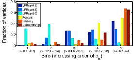
(d) Fraction of vertices with a specific range of internal clustering

coefficient ($c_{in}$) in LFR and real-world networks.

Figure 1: (Color online) Toy examples and empirical observations demonstrating the drawbacks of existing community scoring metrics. The communities in (a) and (c) are distinguished by different colors.

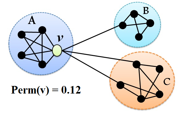
Figure 2: Toy example depicting permanence of a vertex $v$ (here $I(v)$=4, $D(v)$=7, $E_{max}(v)$=2, $c_{in}(v)$=$\frac{5}{6}$).

2.3 Formulation of Permanence

Based on our observations on the distribution of external connections and the internal clustering coefficient, we formulate permanence of a vertex based on the following two criteria that measure the possibility of the vertex remaining in its own community:

(i) The internal connections, $I(.)$, of the vertex $v$ should be more than the maximum connections to a single external community, $E_{max}(.)$, which results more internal pull than the maximum external pull. This criteria is represented in the permanence computation as the ratio of $I(v)$ and $E_{max}(v)$ (indicated by F1 in Equation 1). If the vertex has no external connections, F1 is just the value of the internal connections. We normalize this value by the total degree of the vertex, $D(v)$ (indicated by F2 in Equation 1), which ensures that the product of F1 and F2 will be between 0 (no internal connections) and 1 (no external connections).

(ii) Within a specific community, the internal neighbors of the vertex $v$ should be highly connected among each other (i.e., its internal clustering coefficient, $c_{in}(v)$, should be high). This criteria emphasizes that a vertex is likely to be within a community if it is part of a near-clique substructure. For computing $c_{in}(v)$, we assume that each community should have at least three vertices and three internal connections; otherwise, $c_{in}(v)$ is set to 0. When computing permanence, we impose a penalty based on low internal clustering coefficient (indicated by F3 in Equation 1). The less the internal clustering coefficient, the more the penalty imposed to the final outcome of the community score. This value also ranges from 0 (no penalty) to 1 (maximum penalty).

We aggregate these two criteria to formulate permanence of a vertex $v$ as follows:

$$Perm(v)=\Big{[}\underbrace{\frac{I(v)}{E_{max}(v)}}_{\text{F1}}\times\underbrace{\frac{1}{D(v)}}_{\text{F2}}\Big{]}-\Big{[}\underbrace{1-c_{in}(v)}_{\text{F3}}\Big{]}$$ (1)

Figure 2 depicts a toy example for measuring permanence of a vertex $v$. Note that, this formula actually differentiates between the two cases in Figure 1(a) with higher permanence value for the case where the external pull is uniform. Similarly, the formula differentiates between the two cases in Figure 1(c) by imposing more penalty on the network that has a less tightly knit internal substructure.

2.4 Boundary Conditions of Permanence

For vertices that do not have any external connections, $Perm(v)$ is considered to be equal to the internal clustering coefficient (i.e., $Perm(v)=c_{in}(v)$). The maximum value of $Perm(v)$ is 1 and is obtained when vertex $v$ is an internal node and part of a clique. The lower bound of $Perm(v)$ is close to -1. This is obtained when $I(v)\ll D(v)$, such that $\frac{I(v)}{D(v)E_{max}(v)}\approx 0$ and $c_{in}(v)=0$. Therefore for every vertex $v$, $-1<Perm(v)\leq 1$. The permanence of a graph $G(V,E)$, where $V$ is the set of vertices and $E$ is the set of edges, is given by $Perm(G)=\frac{1}{|V|}\sum_{v\in V}Perm(v)$. For a graph $G(V,E)$, the range is $-1<Perm(G)\leq 1$.

$Perm(G)$ will be closer to 1 as more vertices have high permanence, that is more vertices are in well-defined communities. This can happen only if the network has a strong community structure. The maximum value obtained is when $G$ consists of a series of disconnected cliques. If there is a vertex bridging between two cliques, then the highest overall permanence will be obtained if each clique acts as a separate community and bridging vertex forms a singleton community. For a grid, the best value of $Perm(G)$ will be zero, i.e., each vertex is assigned to a singleton community.

3 Experimental Setup

In this section, we provide a brief overview of the datasets, metrics and comparative methods that we use for our experiments.

3.1 Test Suite of Networks

We use the LFR benchmark model [15] to generate synthetic networks along with their ground-truth communities. Users can specify the following properties: number of nodes ($n$), average ($<k>$) and maximum ($k_{max}$) degree, the degree distribution, the community size distribution, and the mixing-coefficient ($\mu$). The mixing coefficient represents the ratio (in average) between the external connections of a node to its degree. Thus the lower the value of $\mu$, the stronger the community in the network. For our experiments, we set the number of nodes as 1000, and $\mu$ as 0.1, 0.3 and 0.6 (unless mentioned otherwise). For the rest of the parameters, we use the default values mentioned in the authors’ implementation [15].

We also use three real-world networks whose true community structures are known a-priori and whose properties are summarized in Table 1.
Football network was proposed by Girvan and Newman [10] which contains the network of American football games between Division IA colleges during regular season Fall of 2000. The vertices in the graph represent teams (identified by their college names), and edges represent regular-season games between the two teams they connect.
Indian Railway network proposed by Ghosh et al. [9] consists of nodes representing stations, where two stations $s_{i}$ and $s_{j}$ are connected by an edge if there exists at least one train-route such that both $s_{i}$ and $s_{j}$ are scheduled halts on that route. The weight of the edge between $s_{i}$ and $s_{j}$ is the number of train-routes on which both these stations are scheduled halts. We filter out the low-weight edges and then make the resultant network unweighted. We tag each station based on the state in India to which that station belongs. The states act as communities since the number of trains within each state is much higher than the number of trains between two states.
Co-authorship network is derived from the citation dataset developed by Chakraborty et al. [4]. This dataset contains the metadata (title, author(s), related field(s) of the paper, publication venue, year of publication, references and abstract) of all the papers of computer science published between 1960 to 2009 and archived in DBLP repository. We build an aggregated undirected coauthorship network where each node represents an author, and an undirected edge between a pair of authors is drawn if they were co-authors at least once. Since each paper is marked by its related field, we assume this field as the research area of the author(s) writing that paper. Therefore, an author may possess more than one area of research interests. We resolve this by tagging each author by the major field on which she has written most of the papers. These fields act as the ground-truth communities. Besides the aggregated network, we also create some intermediate networks mentioned in Table 8 by cumulatively aggregating all the vertices and edges over each year, e.g., 1960-1971, 1960-1972, …, 1960-1980.

Note that, the principles for constructing the Indian railway network and the co-authorship network are the same – there is an underlying bipartite structure in each case; for railway network, it is the station-train interaction network with an edge denoting if a particular train passes through a station, while for the co-authorship network it is the article-author interaction network with an edge denoting the authorship of a researcher in a scientific article. The railway network is therefore the one-mode projection of the train-station network and the co-authorship network is similarly the one-mode projection of the article-author network. Note that, although the principles of construction are same for both the networks (one clique per train/article is imposed in the one-mode projection), the results, as we shall see in Section 6 are far better for the railway network since the ground-truth here is much more fine-grained in comparison to the co-authorship network.

Table 1: Properties of real-world networks; $n$ and $e$ are the number of nodes and edges, $c$ is the number of communities, <$k$> and $k_{max}$ its average and maximum degree, $n_{c}^{min}$ and $n_{c}^{max}$ the sizes of its smallest and largest communities.

Networks	$n$	$e$	<$k$>	$k_{max}$	$c$	$n_{c}^{min}$	$n_{c}^{max}$
Football	115	613	10.57	12	12	5	13
Railway	301	1224	6.36	48	21	1	46
Coauthorship	103677	352183	5.53	1230	24	34	14404

Table 2: For football network, the values of the scoring functions on the output obtained from different algorithms and the scores of the validation metrics with respect to the ground-truth communities. The ranks of the algorithms (using dense ranking) are shown within parenthesis. The average ranks of all the normal (weighted) validation measures are shown in column 9 (column 13).

Algorithms	Mod	Perm	1-Con	1-Cut	NMI	ARI	PU	Avg	W-NMI	W-ARI	W-PU	Avg
								(N)				(W)
Louvain	0.60(1)	0.36(1)	0.77(5)	0.44(5)	0.93(1)	0.99(1)	0.89(2)	1.33	0.99(2)	0.93(2)	0.99(1)	1.67
FastGreedy	0.58(2)	0.25(3)	0.81(3)	0.59(3)	0.93(1)	0.99(1)	0.91(1)	1.00	1.00(1)	0.94(1)	0.99(1)	1.00
CNM	0.55(3)	0.20(4)	0.85(1)	0.86(1)	0.67(4)	0.75(4)	0.42(5)	4.33	0.55(5)	0.63(5)	0.71(3)	4.33
WalkTrap	0.60(1)	0.36(1)	0.82(2)	0.69(2)	0.90(2)	0.98(2)	0.84(3)	2.33	0.98(3)	0.91(3)	0.99(1)	2.33
Infomod	0.60(1)	0.35(2)	0.82(2)	0.69(2)	0.89(3)	0.97(3)	0.82(4)	3.33	0.97(4)	0.89(4)	0.98(2)	3.33
Infomap	0.60(1)	0.35(2)	0.79(4)	0.51(4)	0.89(3)	0.97(3)	0.82(4)	3.33	0.97(4)	0.89(4)	0.98(2)	3.33

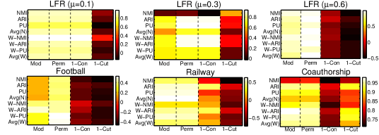
Figure 3: (Color online) Heat maps depicting the pairwise Spearman’s rank correlation between four scoring functions with six validation measures for six different networks. Avg(N) and Avg(W) are the averages of the ranks of three normal and three weighted validation measures respectively as shown in Table 2.

3.2 Scoring Functions for Evaluating Community Structure

The goodness of a community is often measured by how well certain scoring functions are optimized. Here we compare the optimal value of permanence for the obtained communities versus three popular scoring functions, namely modularity (Mod) [21], conductance (Con) [18] and cut-ratio (Cut) [19]. In order to make the higher the better, we measure (1-Con) and (1-Cut) for conductance and cut-ratio respectively.

3.3 Metrics to Compare with Ground-truth

A stronger test of the correctness of the community detection algorithm, however, is by comparing the obtained community with a given ground-truth structure. We use three standard validation metrics, namely Normalized Mutual Information (NMI) [7], Adjusted Rand Index (ARI) [12] and Purity (PU) [20] to measure the accuracy of the detected communities with respect to the ground-truth community structure. [14] argues that these measures have certain drawbacks in that they ignore the connectivity of the network. We therefore also use the weighted versions of these measures, namely Weighted-NMI (W-NMI), Weighted-ARI (W-ARI) and Weighted-Purity (W-PU) as proposed in [14]. Note that, all the metrics are bounded between 0 (no matching) and 1 (perfect matching).

3.4 Community Detection Algorithms

We use the following community detection algorithms for comparison with our proposed algorithm discussed in Section 6:
(i) Modularity-based: FastGreedy [22], Louvain [3] and CNM [6].
(ii) Random walk-based: WalkTrap [24].
(iii) Compression-based: InfoMod [25] and InfoMap [26].

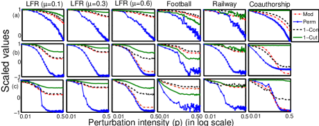
Figure 4: (Color online) Change in the value of the scoring functions with the increase of perturbation intensity ($p$) in (a) edge-based, (b) random and (c) community-based perturbation strategies. The values are normalized by the maximum value obtained from each function.

4 Permanence as a Community
Scoring Function

In this section, we demonstrate the effectiveness of permanence as a scoring function for evaluating the goodness of detected communities, and compare it with modularity, 1-Con and 1-Cut. To do this, we perform the following experiment, on the same lines as that of [27].

These are the steps in our experiment: (i) We apply several community detection algorithms on a specified network and obtain the vertex-to-community assignment as given by each algorithm; (ii) We compute the values of all the community scoring functions for these communities; (iii) For each scoring function we rank the algorithms based on which one of these produces the most optimal (highest) value; (iv) We then compare the obtained community with the known ground-truth community and compute the respective validation measures, namely NMI, ARI, Purity and their weighted versions; (v) For each validation metric, we rank the algorithms based on the one that produces the highest value, i.e., best match with ground-truth.

Table 2 shows the results of the experiment performed on football network. Scoring functions (columns 2-5) are measures of goodness of the community set obtained. The validation metrics (columns 6-8, 10-12) measure the concurrence of the communities with the ground-truth communities. We posit that since these two types of measures are orthogonal, and because the validation metrics generally provide a stronger measure of correctness after measuring similarity with the ground-truth structure, the values of a good scoring function should “match" those of the validation metrics. That is, if a scoring function indeed identifies the correct communities, then when its value is high (low), the values of the corresponding validation metrics would also be high (low).

To compute this correlation, we compare the relative ranks, because the range of the values is not commensurate across the quantities and we are more interested in observing the “up" or “down" direction, rather than the absolute values. For each network, we measure the Spearman’s rank correlation between all pairs of scoring functions and validation measures. Note that, it is not always possible to assign ranks uniquely. We used different ranking schemes to break ties. Here, we present the results using dense ranking; we have also used standard competition ranking and fractional ranking (see in [1]) and our results are consistent across all the different methods.

Results. Table 2 shows the values and ranks for the different metrics for football network. For all the networks, the rank correlations of the scoring functions and the validation metrics are shown as heat maps in Figure 3. Lighter color indicates higher correlation and hence more similarity between the scoring function and the validation metric. For the networks having distinct community structure such as LFR ($\mu=0.1$), football and railway networks, permanence shows comparable performance as that of other scoring functions. However for LFR network, with the increase of $\mu$, the inter-community connection density starts increasing, and it is difficult for any community detection algorithm and/or scoring function to capture the ground-truth communities. Interestingly, we observe that the rank correlation obtained through the permanence scores and those through validation metrics is exceptionally high for LFR ($\mu=0.6$) and coauthorship networks which seem to have poor community structure compared to the other networks (see Table 1 and Table 5). Since the ground-truth communities are not well formed, there is a wide variance in the type of community structures identified by different algorithms. Permanence score can capture this variability much better than other scoring functions. To summarize the results, in Table 3 we present the average rank correlations of these community scoring functions across all the validation metrics for each network. We observe that for all the networks, permanence on an average produces the best ranking followed by modularity, conductance and cut-ratio in order.

Table 3: Average rank correlations (over different validation metrics) of the community scoring functions for all the networks. For each network, the highest (best) correlation is in bold font.

Networks	Modularity	Permanence	Conductance	Cut
LFR($\mu$=0.1)	0.88	0.88	0.88	0.02
LFR($\mu$=0.3)	0.61	0.74	0.72	0.28
LFR($\mu$=0.6)	0.87	0.96	-0.18	-0.44
Football	0.25	0.43	-0.29	-0.41
Railway	0.43	0.46	0.08	-0.48
Coauthorship	0.92	0.92	0.76	0.86

5 Sensitivity of Permanence

We now evaluate the sensitivity of permanence under different perturbations of the ground-truth community structure. We posit that a good metric for evaluating communities should be stable under small perturbations of the ground-truth communities (i.e., groups of nodes that differ very slightly from the ground-truth communities). This indicates that the scoring function is robust to noise. However, if the perturbation is beyond a threshold, i.e., when the ground-truth community structure is perturbed to such an extent that it resembles a random set of nodes, then a good scoring function should assign it a low score.

Given a graph $G=<V,E>$ and perturbation intensity $p$, we start with the ground-truth community $S$ and then modify it (i.e., change its members) by executing the perturbation strategy $p\cdot m$ times. The value of $m$ is based on different strategies, as described below. For our experiments, we adopt three perturbation strategies motivated by the methods proposed in [28]:

(i)Edge-based perturbation picks a random inter-comm-unity edge $(u,v)$ where $u\in S$ and $v\in S^{\prime}$ (where $S\neq S^{\prime}$) and then swaps the memberships (i.e., assign $u$ to $S^{\prime}$ and $v$ to $S$). It continues until $p\cdot|E|$ iterations are completed (here, $m=|E|$). This strategy preserves the size of $S$. However, if $v$ is not connected to any other nodes in $S$ except $u$, then it makes $S$ disconnected.

(ii) Random perturbation takes community members and replaces them with random non-members. We pick two random nodes $u\in S$ and $v\in S^{\prime}$ (where $S\neq S^{\prime}$) and then swap their memberships. It continues until $p\cdot|V|$ iterations are completed (here, $m=|V|$). Random perturbation maintains the size of $S$ but may disconnect $S$. Generally, it degrades the quality of $S$ faster than edge-based strategy, since edge-based strategy only affects the “fringe” of the community.

(iii) Community-based perturbation adopts a similar mechanism as in the edge-based strategy. However, it considers each community $S$ from the ground-truth community structure one by one and continues the perturbation until $p\cdot|S|$ constituent nodes of the community are swapped with the other non-constituent nodes (here, $m=|S|$). This process is repeated for all the communities separately. This perturbation decreases the quality of the ground-truth communities the fastest among the three since the number of swaps is much higher than the others.

We perturb different networks using these three perturbation strategies for values of $p$ ranging between 0.01 to 0.5. We compute the values of four community scoring functions, i.e., modularity, permanence, 1-Con and 1-Cut. For small values of $p$, small change of the original value of the scoring function is desirable since it indicates that the scoring function is robust to noise. For high perturbation intensities (i.e., for larger values of $p$), the value should drop significantly since the communities become more random.

Results. Figure 4 shows the results of our experiments. For a commensurate comparison, we rescale the values of each parameter by normalizing with the maximum value obtained from that function. For all three strategies, the values of the scoring functions tend to decrease with the increase of $p$, and the effect is most prominent in community-based strategy followed by random and edge-based strategies. For each network, once $p$ has reached a certain threshold, the decrease is much faster in permanence. On more careful inspection, we find that this happens because the internal structure of a community completely breaks down if perturbation is taken beyond a point and thus has an avalanche effect on the value of the clustering coefficient ($c_{in}(v)$ in Equation (1)). This in turn quickly pulls the value of permanence down. Summarizing, the results indicate that permanence is a better measure for distinguishing true communities from randomized sets of nodes than the other parameters.

6 Permanence Maximization

Inspired by the effectiveness of permanence as a scoring function and its sensitivity to perturbations, we develop a community detection algorithm called Max_Permanence (pseudocode in Algorithm 1) that identifies communities by maximizing permanence.

Our algorithm is a heuristic, that strives to obtain a high value of permanence. In this algorithm, we begin with initializing every vertex to a singleton community. A vertex is moved to a community only if this movement results in a net increase in the number of internal connections and/or a net decrease in the number of external connections to any of the neighboring communities. If such a move is not possible, then either the vertex remains as a singleton (such as in the case where moving to any one of the candidate communities will give equal permanence) or moves to the community where it is more tightly connected with its neighbors (this causes the vertex to have positive permanence). This process is repeated for each vertex and the entire relocation of all vertices is repeated over several iterations until the permanence value converges. However, convergence is not theoretically guaranteed, but we observed that the algorithm converges with high probability.

Algorithm 1 Max_Permanence

Input: A graph $G$.
Output: Permanence of $G$; Detected communities

procedure Max Permanence($G(V,E)$)

    Each vertex is assigned to its seed community

    Set value of maximum iteration as $maxIt$

    $vertices\leftarrow|V|$

    $Sum\leftarrow 0$

    $Old\_Sum\leftarrow-1$

    $Itern\leftarrow 0$

    while $Sum\neq Old\_Sum$ and $Itern<maxIt$ do

       $Itern\leftarrow Itern+1$

       $Old\_Sum\leftarrow Sum$

       $Sum\leftarrow 0$

       for all $v\in V$ do

               (compute current permanence of $v$)

          $cur\_p\leftarrow Perm(v)$

          if $cur\_p==1$ then

             $Sum\leftarrow Sum+cur\_p$

                     continue;

          

          $cur\_p\_neig\leftarrow 0$ $\triangleright$ $Neig(v)$=set of neighbors of $v$

          for all $u\in Neig(v)$ do

                    (compute current permanence of $u$)

             $cur\_p\_neig\leftarrow cur\_p\_neig+Perm(u)$           

$\triangleright$ $Comm(v)$ is the set of neighboring communities of $v$

          for all $C\in Comm(v)$ do 

             Move $v$ to community $C$

                     (compute permanence of $v$ in community $C$)

             $n\_p\leftarrow Perm(v)$

$\triangleright$ Neighbors of $v$ are affected for this movement

             $n\_p\_neig\leftarrow 0$

             for all $u\in Neig(v)$ do

                    (compute new permanence of $u$)

                $n\_p\_neig\leftarrow n\_p\_neig+Perm(u)$              

             if ($cur\_p<n\_p)$ and ($cur\_p\_neig<n\_p\_neig)$ then

                $cur\_p\leftarrow n\_p$

             else

                          replace $v$ to its original community                        

          $Sum\leftarrow Sum+cur\_p$            

    $Netw\_perm=Sum/vertices$ $\triangleright$ Permanence of $G$

    return $Netw\_perm$

Table 4: Improvement of Max_Permanence with respect to the average (left-hand value) and the best (right-hand value) performances of the six competing algorithms (separated by semicolon). Positive (negative) values indicate that Max_Permanence outperforms (underperforms) the corresponding performances of the competing algorithms.

Validation metrics	LFR ($\mu$=0.1)	LFR ($\mu$=0.3)	LFR ($\mu$=0.6)	Football	Railway	Coauthorship
NMI	0.04;   0.00	0.15;  0.05	-0.31;  -0.78	0.04;  0.00	0.15;  0.11	0.04;  -0.06
ARI	0.06;  0.00	0.21;   0.02	-0.39;   -0.76	0.07;   0.00	0.03;   0.04	0.03;   -0.08
PU	0.04;  0.00	0.17;   0.00	-0.38;   -0.72	0.01;   0.00	0.13;   0.00	0.03;   -0.06
W-NMI	0.02;  0.00	0.14;   0.00	-0.41;   -0.78	0.09;   0.00	0.26;   0.00	0.05;   -0.01
W-ARI	0.05;  0.02	0.19;   0.05	-0.35;   -0.72	0.05;   0.00	0.02;   -0.15	0.04;   -0.06
W-PU	0.03;  0.01	0.17;   0.00	-0.45;   -0.79	0.00;   0.00	0.05;   -0.04	0.02;   -0.15

6.1 Performance Evaluation

Table 4 shows results of the improvement of our method (as differences) compared to the average and best performances of six competing algorithms (given in Section 3.4) based on six ground-truth based validation metrics.

Comparable results - in LFR ($\mu$ = 0.1) and football networks, since the communities are well-separated, most algorithms efficiently capture these partitions and our method is comparable to the other algorithms as well.

Improved results - in LFR ($\mu=0.3$) and railway networks, our method significantly outperforms other algorithms. Moreover in railway network, we observe that our algorithm detects three singleton communities (i.e., communities each containing only one vertex), one of which is also present in the ground-truth structure. None of the community detection algorithms is able to capture this singleton community.

Moderate results - our method does not work well for the LFR ($\mu=0.6$) network. For coauthorship network, we observe that though our algorithm outperforms the average performance of the competing algorithms, it performs less well than that of the two information-theoretic approaches (Infomod and Infomap).

Reasons behind moderate performance
LFR ($\mu$=0.6) – To understand why our algorithm is not as competitive for LFR ($\mu=0.6$), we further observe the quality of the ground-truth communities in three LFR networks. We observe that while the average internal clustering coefficient of vertices in LFR ($\mu=0.1$) is 0.78, it deteriorates to 0.36 for LFR ($\mu=0.6$). Moreover, 97% of vertices in ground-truth communities of LFR ($\mu$=0.6) have less internal connections than the external connections (while LFR ($\mu$=0.1) and LFR ($\mu$=0.3) hardly have any such nodes). This indicates that LFR ($\mu=0.6$) does not have modular structure in the ground-truth communities.

To further strengthen this claim, we also measure the similarity of the communities obtained by different community detection algorithms (as listed in Section 3.4) across different validation measures. The results in Table 5 clearly show the degradation of the similarity values with the increase in $\mu$. The reason is that with the increase in $\mu$, the communities in LFR network tend to be less well-knit, and thus the agreement of the outputs of different algorithms is also less. Therefore, the output of a good community detection algorithm should reflect such absence of modular structure in the network (hence shows poor performance).
Coauthorship network – To explain the permanence-based results obtained from coauthorship network, we further analyze the communities obtained from our algorithm. We check the title and the abstract of the papers written by the authors in each community of coauthorship network, and notice that our method splits large ground-truth communities into denser submodules. This splitting is mostly noticed in older research areas such as Algorithms and Theory, Databases etc. These submodules are actually the subfields (sub-communities) of a field (community) in computer science domain. Few examples of such sub-communities obtained from our algorithm are noted in Table 6. Thus, our algorithm, in addition to identifying well-defined communities, is also able to unfold the hierarchical organization of a network.

Table 5: Average values among pairwise similarities between outputs of the community detection algorithms on different LFR networks.

Validation	LFR	LFR	LFR
measures	($\mu$=0.1)	($\mu$=0.3)	($\mu$=0.6)
NMI	0.95	0.82	0.53
ARI	0.98	0.79	0.48
PU	0.99	0.85	0.56
W-NMI	0.94	0.85	0.54
W-ARI	0.97	0.78	0.50
W-PU	0.98	0.83	0.57

Table 6: Example of communities and sub-communities obtained from coauthorship network using Max_Permanence algorithm.

Communities	Sub-communities
Algorithms	Theory of computation; Formal methods; Data structure;
and Theory	Information & coding theory; Computational geometry
Databases	Models; Query optimization; Database languages;
	storage; Performance, security, and availability

Comparison of largest community size. Many optimization algorithms have the tendency to underestimate smaller size communities (known as the resolution limit problem [11]) and sometimes tend to produce very large size communities. In our test suite, we observe the similar tendency in all the competing algorithms whereas the communities obtained by permanence are smaller in size. In Table 7, we show for two representative networks that the size of the largest communities detected by the other algorithms is much larger than the size of the largest community present in the ground-truth structure. We also measure the maximum similarity (using Jaccard coefficient) between the largest-size community detected by each algorithm with the communities in ground-truth structure and notice that Max_Permanence is able to detect largest size community which is most similar to the ground-truth structure. Therefore, we hypothesize that our algorithm has the potentiality to reduce the effect of resolution limit.

Table 7: Size of the largest communities obtained from different community detection algorithms and their similarities with the ground-truth structure for two networks (LFR ($\mu$=0.3, N=1000) and football).

	Largest community size		Similarity
	LFR	Football	LFR	Football
	($\mu=0.3$)		($\mu=0.3$)
Ground-truth	49	12	–	–
Louvain	62	24	0.70	0.41
FastGreedy	95	18	0.32	0.65
CNM	91	32	0.52	0.31
Walktrap	83	15	0.51	0.57
Infomod	61	16	0.79	0.86
Infomap	59	16	0.74	0.86
Max_Permanence	49	13	1	0.92

6.2 Handling Modularity Maximization Issues

As discussed earlier, modularity maximization algorithms suffer from the issues including (a) resolution limit, (b) degeneracy of solution and (c) dependence on the size of the graph [11]. We now discuss how each of these problems are ameliorated by maximizing permanence.

We demonstrate that community assignments are different in a modularity-based algorithm vis-a-vis Max_Permanence algorithm using the example in Figure 5. In this figure, we assume that apart from the edges through $v$, there is no connection between the communities $A$ and $B$.

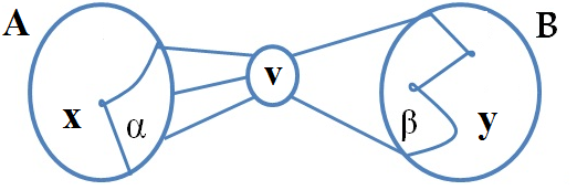
Figure 5: (Color online) An illustrative example to show the community assignment of vertex $v$.

Table 8: Change in scoring functions with the (near-)symmetric growth of coauthorship network obtained in each year by adding vertices and edges till that year. $N$: number of nodes, $c$: number of communities, $<I>$: average internal degree, $<k>$: average degree, $<c_{in}>$: average internal clustering coefficient, $<E_{max}>$: average maximum external connectivity. The value of permanence is less affected by the growth.

Coauthorship	Year		60-71	60-72	60-73	60-74	60-75	60-76	60-77	60-78	60-79	60-80
	Network	$n$	964	1515	1991	2681	3386	4836	6284	7814	9001	10386
	properties	$c$	24	24	24	24	24	24	24	24	24	24
		$\frac{<I>}{<k>}$	0.082	0.095	0.093	0.091	0.089	0.104	0.111	0.112	0.115	0.113
		$\frac{1}{<E_{max}>}$ ($\times 10^{-4}$)	3.8	3.2	2.9	3.9	2.8	2.11	2.39	2.92	2.69	3.22
		$<(1-c_{in})>$	0.239	0.248	0.246	0.251	0.251	0.260	0.265	0.269	0.270	0.274
	Modularity		0.369	0.374	0.395	0.392	0.421	0.422	0.465	0.471	0.493	0.501
	Permanence		0.094	0.092	0.092	0.096	0.095	0.095	0.097	0.097	0.097	0.098

Terminology. Let vertex $v$ be connected to $\alpha$ ($\beta$) nodes in community $A$ ($B$), and these $\alpha$ ($\beta$) nodes form the set $N_{\alpha}$ ($N_{\beta}$). The number of vertices in community $A$ is ($x+\alpha$), and in community $B$ is ($y+\beta$). Let the average internal degree of a vertex $a\in N_{\alpha}$ and a vertex $b\in N_{\beta}$, before $v$ is assigned to any of the communities, be $I_{\alpha}$ and $I_{\beta}$ respectively. Let the average internal clustering coefficient of the neighboring nodes in communities $A$ and $B$ be $C_{A}$ and $C_{B}$ respectively. If $v$ is added to communities $A$ ($B$) then the average internal clustering coefficient of $v$ becomes $C^{v}_{A}$ ($C^{v}_{B}$), and the average internal clustering coefficient of the nodes in $N_{\alpha}$($N_{\beta}$) become $C^{\alpha}$ ($C^{\beta}$).

We assume that the communities $A$ and $B$ are tightly connected internally such that the values of $C_{A}$ and $C_{B}$ are very high (> 0.5). To simplify the explanations, we consider the case where none of the neighbors of $v$ are connected to each other. If $v$ does not add any new edges to the group of neighbors, then $C^{\alpha}=C_{A}\frac{(I_{\alpha}-1)}{(I_{\alpha}+1)}$ (similarly, $C^{\beta}=C_{B}\frac{(I_{\beta}-1)}{(I_{\beta}+1)}$).

Given this scenario, we can determine the conditions (due to the lack of space detailed calculations are provided in an online appendix [1]) for which a particular assignment of $v$ to any of the communities will give the highest permanence. Using these conditions, we show how permanence overcomes some of the issues related to modularity maximization.

Degeneracy of solution is a problem where a community scoring function (e.g., modularity) admits multiple distinct high-scoring solutions and typically lacks a clear global maximum, thereby, resorting to tie-breaking [11]. For our example, when $\alpha$ = $\beta$, modularity maximization algorithm will assign $v$ arbitrarily to $A$ or $B$. However, in the case of permanence, $v$ will remain as a separate community so long as the following condition is maintained:

Condition. If $\alpha=\beta$, $C^{\beta}=C_{B}\frac{I_{\beta}-1}{I_{\beta}+1}$, then communities $A$, $B$ and $v$ will remain separate rather than $v$ joining community $A$, if $\alpha(\frac{2C_{A}-1}{I_{\alpha}+1})+(1-C^{v}_{A})\geq\frac{1}{2\alpha}$.

We observe that when $\alpha=\beta=1$, then $C^{v}_{A}=0$ and the communities will always remain separate. Furthermore, as $\alpha$ increases, the left-hand side of the above condition will become larger than the right, thus increasing the chance of separate communities.

Resolution limit is a problem where communities of certain small size are merged into larger ones [11]. A classic example where modularity cannot identify communities of small size is a cycle of $m$ cliques. Here maximum modularity is obtained if two neighboring cliques are merged.

In the case of permanence, we can determine that whether two communities $A$ and $B$ would merge (as in modularity) or whether $v$ would join community $A$ (we select $A$, but similar analysis can also be done for the case when $v$ joins $B$), by the following condition:

Condition. Joining $v$ to community $A$ gives higher permanence than merging the communities $A$, $B$ and $v$ if $C^{\beta}=C_{B}$, and ($\frac{\gamma}{(\gamma+1)\beta}+\frac{C^{v}_{A}(2\gamma+1)-C^{v}_{B}}{(\gamma+1)^{2}}-\frac{\beta}{I_{\beta}+1}$)>1; where $\gamma=\alpha/\beta$ and also if $C^{\beta}=C_{B}\frac{I_{\beta}-1}{I_{\beta}+1}$, and $(\frac{\gamma}{(\gamma+1)\beta}+\frac{C^{v}_{A}(2\gamma+1)-C^{v}_{B}}{(\gamma+1)^{2}}+\frac{\beta(2C_{B}-1)}{I_{\beta}+1})>1$.

This result is independent of the size of the communities. Moreover, so long as $A$ and $B$ are almost cliques (internal clustering coefficients > 0.5), $C^{v}_{A}$ is sufficiently high and $C^{v}_{B}$ is sufficiently small (e.g., $C^{v}_{A}$ >2/3 and $C^{v}_{B}$=0), $v$ will join community $A$ rather than merging. Thus, in general, the highest permanence is obtained if $v$ joins the community to which it is very tightly connected rather than the one to which it is loosely connected.

Asymptotic growth of value of a metric implies a strong dependence on the size of the network and the number of modules the network contains [11]. Rewriting Equation 1, we get the permanence of the entire network $G$ as follows: $Perm(G)=\frac{1}{|V|}\sum_{v\in V}\left[\frac{I(v)}{D(v)E_{max}(v)}\right]-\frac{1}{|V|}\sum_{v\in V}\left[(1-c_{in}(v))\right]$. We can notice that most of the parameters in the above formula are independent of the network size and the number of communities. Table 8 illustrates the change in modularity and permanence with the symmetric growth of the network size in coauthorship network. Note that, the intermediate networks are formed by cumulatively aggregating all the vertices and edges of coauthorship network over the years, e.g., 1960-1971, 1960-1972,…, 1960-1980. We observe that the modularity increases consistently with the symmetric growth, while the value of permanence remains almost constant.

7 Related Work

A huge volume of work has been devoted to finding communities in large networks, including diverse methods such as modularity optimization [3, 6], spectral graph-partitioning [23], random-walk [24], information-theoretic [25, 26], consensus clustering [17] and many others (see [8] for the review). Recently, Chakraborty et al. [5] pointed out how vertex ordering influences the results of the community detection algorithms. They identify invariant groups of vertices (named as “constant communities”) whose assignment to communities are not affected by vertex ordering.

On the other hand, several metrics for evaluating the quality of community structure have been proposed. The most popular is modularity [21]. However, community detection using modularity has certain issues including resolution limit, degeneracy of solutions and asymptotic growth [11]. To address these issues, multi-resolution versions of modularity [2] were proposed to allow researchers to specify a tunable target resolution limit parameter. Furthermore, Lancichinetti and Fortunato [16] stated that even those multi-resolution versions of modularity are not only inclined to merge the smallest well-formed communities, but also to split the largest well-formed communities.

8 Discussions and Future work

In this paper, we have introduced a new vertex-based metric, permanence for evaluating the goodness of communities in networks. From our experiments we observe that the permanence score has a good correlation with the quality of the ground-truth communities (Section 4) and is sensitive to perturbations in the community structure (Section 5). In addition, permanence also provides some significant advantages compared to other popular community scoring functions.

The value of permanence strongly correlates to the community like structure of the network. For example, the power grid network, which is not at all modular [13], has a modularity of 0.98 and a permanence of -0.16. In contrast, community-rich networks such as a circle of 30 cliques generate permanence (modularity) of 0.92 (0.87). Therefore, permanence can also be used to identify whether the network is at all suitable for community detection.

We believe that the advantages of permanence arise because it is a local vertex-based metric as opposed to the more common global/mesoscopic metrics. At the same time, permanence also derives the benefits of a global metric to a certain extent by looking into the exact community assignments of the external neighbors of the vertex considered. Perfectly global metrics tend to aggregate the effect of the connections of all the vertices in a community. As we have seen in Section 2 we can lose information by aggregation, particularly if the distribution of the connections is skewed. A vertex-based metric is more fine-grained, and therefore allows partial estimation of communities in a network whose entire structure is not known.

In this paper we have empirically demonstrated the advantages of permanence. As an immediate future work, we plan to extend permanence metric to evaluate the quality of overlapping communities and communities in dynamic and weighted networks. We believe that this metric will help in formulating a strong theoretical foundation for identifying community structures where the ground-truth is not known. All the codes, datasets and supporting materials are publicly available at http://cnerg.org/permanence/.

9 Acknowledgments

The first author of the paper is financially supported by Google India PhD Fellowship Grant for Social Computing. The authors from University of Nebraska are supported by College of IS&T, the Graca grant for UNO-SPR and the RISC Fellowship.

References

- [1] http://cse.iitkgp.ac.in/resgrp/cnerg/Files/resources/appendix_permanence.%pdf.
- [2] A. Arenas, A. Fernández, and S. Gómez. Analysis of the structure of complex networks at different resolution levels. New Journal of Physics, 10(5):053039, 2008.
- [3] V. D. Blondel, J.-L. Guillaume, R. Lambiotte, and E. Lefebvre. Fast unfolding of communities in large networks. J. Stat. Mech., 2008(10):P10008, Oct. 2008.
- [4] T. Chakraborty, S. Sikdar, V. Tammana, N. Ganguly, and A. Mukherjee. Computer science fields as ground-truth communities: Their impact, rise and fall. In ASONAM, pages 426 – 433, 2013.
- [5] T. Chakraborty, S. Srinivasan, N. Ganguly, S. Bhowmick, and A. Mukherjee. Constant Communities in Complex Networks. Scientific Reports, 3, May 2013.
- [6] A. Clauset, M. E. J. Newman, and C. Moore. Finding community structure in very large networks. Phys. Rev. E, 70(6):066111, 2004.
- [7] L. Danon, A. Diaz-Guilera, J. Duch, and A. Arenas. Comparing community structure identification. J. Stat. Mech., 9:P09008, 2005.
- [8] S. Fortunato. Community detection in graphs. Phys. Rep., 486:75–174, 2010.
- [9] S. Ghosh, A. Banerjee, N. Sharma, S. Agarwal, and N. Ganguly. Statistical analysis of the indian railway network: a complex network approach. Acta Physica Polonica B Proceedings Supplement, 4:123–137, 2011.
- [10] M. Girvan and M. E. Newman. Community structure in social and biological networks. PNAS, 99(12):7821–7826, June 2002.
- [11] B. Good, Y. D. Montjoye, and A. Clauset. Performance of modularity maximization in practical contexts. Phys. Rev. E, 81(4):046106, 2010.
- [12] L. Hubert and P. Arabie. Comparing partitions. Journal of classification, 2(1):193–218, 1985.
- [13] B. Karrer, E. Levina, and M. E. J. Newman. Robustness of community structure in networks. Phys. Rev. E, 77(4):046119, 2008.
- [14] V. Labatut. Generalized measures for the evaluation of community detection methods. CoRR, abs/1303.5441, 2013.
- [15] A. Lancichinetti and S. Fortunato. Benchmarks for testing community detection algorithms on directed and weighted graphs with overlapping communities. Phys. Rev. E, 80(1):016118, July 2009.
- [16] A. Lancichinetti and S. Fortunato. Limits of modularity maximization in community detection. Phys. Rev. E, 84:066122, 2011.
- [17] A. Lancichinetti and S. Fortunato. Consensus clustering in complex networks. Scientific Reports, 2, 2012.
- [18] J. Leskovec, K. J. Lang, A. Dasgupta, and M. W. Mahoney. Community structure in large networks: Natural cluster sizes and the absence of large well-defined clusters. Internet Mathematics, 6(1):29–123, 2009.
- [19] J. Leskovec, K. J. Lang, and M. Mahoney. Empirical comparison of algorithms for network community detection. In WWW, pages 631–640, New York, USA, 2010. ACM.
- [20] C. D. Manning, P. Raghavan, and H. Schütze. Introduction to Information Retrieval. Cambridge University Press, New York, NY, USA, 2008.
- [21] M. E. Newman. Modularity and community structure in networks. PNAS, 103(23):8577–8582, June 2006.
- [22] M. E. J. Newman. Fast algorithm for detecting community structure in networks. Phys. Rev. E, 69(6):066133, 2004.
- [23] M. E. J. Newman. Spectral methods for community detection and graph partitioning. Phys. Rev. E, 88:042822, 2013.
- [24] P. Pons and M. Latapy. Computing communities in large networks using random walks. Journal of Graph Algortihms and Applications, 10(2):191–218, 2006.
- [25] M. Rosvall and C. Bergstrom. An information-theoretic framework for resolving community structure in complex networks. PNAS, 104(18):7327, 2007.
- [26] M. Rosvall and C. T. Bergstrom. Maps of random walks on complex networks reveal community structure. PNAS, 105(4):1118–1123, 2008.
- [27] K. Steinhaeuser and N. V. Chawla. Identifying and evaluating community structure in complex networks. Pattern Recog. Lett., 31(5):413–421, 2010.
- [28] J. Yang and J. Leskovec. Defining and evaluating network communities based on ground-truth. In ACM SIGKDD Workshop on Mining Data Semantics, pages 3:1–3:8, New York, USA, 2012.