Position-momentum correlations in matter waves double-slit experiment

Abstract

We present a treatment of the double-slit interference of matter-waves represented by Gaussian wavepackets. The interference pattern is modelled with Green’s function propagator which emphasizes the coordinate correlations and phases. We explore the connection between phases and position-momentum correlations in the intensity, visibility and predictability of the wavepackets interference. This formulation will indicate some aspects that can be useful for theoretical and experimental treatment of particles, atoms or molecules interferometry.

I Introduction

The double-slit experiment illustrates the essential mystery of quantum mechanics Faynman . Under different circumstances, the same physical system can exhibit either a particle-like or a wave-like behaviour, otherwise known as wave-particle duality Bohr . Double-slit experiments with matter waves were performed by Möllenstedt and Jösson for electrons Jonsson , by Zeilinger et al. for neutrons Zeilinger1 , by Carnal and Mlynek for atoms Carnal , by Schöllkopf and Toennies for small molecules Toennies and by Zeilinger et al. for macromolecules Zeilinger2 .

Position-momentum correlations have been studied and interpreted in some textbooks, while the most treated example is the simple Gaussian or minimum-uncertainty wavepacket solution for the Schrödinger equation for a free particle. Such wavepacket presents no position-momentum correlations at $t=0$ which appear only with the passage of time Bohm ; Saxon . How the phases of the wave function influence the existence of position-momentum correlations is also explained in Ref. Bohm . Posteriorly, it was shown that squeezed states or linear combination of Gaussian states can exhibit initial correlations, i.e., correlations that not depend on the time evolution Robinett ; Riahi ; Dodonov ; Campos .

The qualitative changes in the interference pattern as a function of the increasing in the position-momentum correlations was studied in Ref. Carol . In addition, it was shown that the Gouy phase of matter waves is directly related to the position-momentum correlations, as studied by the first time in Refs. Paz1 ; Paz2 . The Gouy phase of matter waves was experimentally observed in different systems, such as Bose-Einstein condensates cond , electron vortex beams elec2 , and astigmatic electron matter waves using in-line holography elec1 . More recently, it was observed that the position-momentum correlations can provide further insight into the formation of above-threshold ionization (ATI) spectra in the electron-ion scattering in strong laser fields Kull .

In this work, we use the previously developed ideas on position-momentum correlations to analyze the Gaussian features of the wavepacket and the interference pattern, as well as the wave-like and particle-like behavior, in double-slit experiment with matter waves. Before reaching the double-slit setup, the particle is represented by a simple Gaussian wavepacket and, after the double-slit apparatus, the particle is represented by a linear combination of two identical Gaussian wavepackets coming from the two slits. After the double-slit, the position and momentum of the particle will be correlated even if the time evolution from the source to the double-slit is zero. The correlations will be changed by the evolution, enabling us to extract some information about the interference pattern.

In section II we present the model for the double-slit experiment considering that the matter wave propagates the time $t$ from the source to the double-slit and the time $\tau$ from the double-slit to the screen. Further, we calculate the wave functions for the passage through each slit using the Green’s function for the free particle. In section III, we calculate the position-momentum correlations and the generalized Robertson-Schrödinger uncertainty relation for the state that is a linear combination of the states which passed through each slit. In section IV, we calculate the intensity, visibility and predictability to analyze the interference pattern in terms of the knowledge of the position-momentum correlations .

II Double-Slit Experiment

In this section we return to the double-slit experiment and analyze the effect of the position-momentum correlations in the interference pattern. We consider that a coherent Gaussian wavepacket of initial width $\sigma_{0}$ propagates during a time $t$ before arriving at a double-slit that divides it into two Gaussian wavepackets. After the double-slit, the two wavepackets propagate during a time $\tau$ until they reach the detection screen, where they are recombined and the interference pattern is observed as a function of the transverse coordinate $x$. As we will see, the number of interference fringes and its quality are dramatically influenced by the propagation times $t$ and $\tau$. In particular, there is a value of time $t_{max}(\tau)$ for which the number of fringes tends to be minimum. This value of time corresponds to a maximum separation of the wavepackets on the screen and it is associated with one maximum of the position-momentum correlations. On the other hand, if the source of particles is positioned in such a way that, before arriving the screen, the particles travel during a time interval which is not close to $t_{max}(\tau)$, the number of interference fringes and its quality are increased significantly.

The wavefunction at the time when the wave passes through the slit $1(+)$ or the slit $2(-)$ is given by

$$\psi_{1,2}(x,t,\tau)=\int_{-\infty}^{+\infty}dx_{j}\int_{-\infty}^{+\infty}dx_{i}G_{2}(x,t+\tau;x_{j},t)F(x_{j}\pm d/2)G_{1}(x_{j},t;x_{i},0)\psi_{0}(x_{i}),$$ (1)

where

$$G_{1}(x_{j},t;x_{i},0)=\sqrt{\frac{m}{2\pi i\hbar t}}\exp\left[\frac{im(x_{j}-x_{i})^{2}}{2\hbar t}\right],$$ (2)

$$G_{2}(x,t+\tau;x_{j},t)=\sqrt{\frac{m}{2\pi i\hbar\tau}}\exp\left[\frac{im(x-x_{j})^{2}}{2\hbar\tau}\right],$$ (3)

$$F(x_{j}\pm d/2)=\frac{1}{\sqrt{\beta\sqrt{\pi}}}\exp\left[-\frac{(x_{j}\pm d/2)^{2}}{2\beta^{2}}\right],$$ (4)

and

$$\psi_{0}(x_{i})=\frac{1}{\sqrt{\beta\sqrt{\pi}}}\exp\left(-\frac{x_{i}^{2}}{2\sigma_{0}^{2}}\right).$$ (5)

The kernels $G_{1}(x_{j},t;x_{i},0)$ and $G_{2}(x,t+\tau;x_{j},t)$ are the free propagators for the particle, the functions $F(x_{j}\pm d/2)$ describe the double-slit apertures which are taken to be Gaussian of width $\beta$ separated by a distance $d$; $\sigma_{0}$ is the transverse width of the first slit, where the packet was prepared, $m$ is the mass of the particle, $t$ ($\tau$) is the time of flight from the first slit (double-slit) to the double-slit (screen). We will also consider that the energy associated with the momentum of the atoms in the $z$-direction is very high, such that we can consider a classical movement of atoms in this direction, with the time component given by $z/v_{z}$. This model is presented in Fig. 1 together with a qualitative illustration of the interference pattern for three different values of time $t$, maintaining $\tau$ constant.

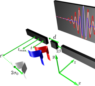
Figure 1: Sketch of double-slit experiment. Gaussian wavepacket of transverse width $\sigma_{0}$ propagates a time $t$ before to attain the double-slit and a time $\tau$ from the double-slit to the screen. The slit aperture are taken to be Gaussian of width $\beta$ and separated by a distance $d$. We also show the qualitative interference pattern considering that the wavepacket propagates the time $t$ (color red), $t_{max}$ (color blue) or $t^{\prime}$ (color purple). For $t_{max}$ we have the minimum of interference fringes.

After some algebraic manipulations, we obtain for the wave that passed though the slit $1$ the following result

$$\psi_{1}(x,t,\tau)=\frac{1}{\sqrt{B\sqrt{\pi}}}\exp\left[-\frac{(x+D/2)^{2}}{2B^{2}}\right]\exp\left(\frac{imx^{2}}{2\hbar R}+i\Delta x+i\theta+i\mu\right),$$ (6)

where

$$B^{2}(t,\tau)=\frac{\left(\frac{1}{\beta^{2}}+\frac{1}{b^{2}}\right)^{2}+\frac{m^{2}}{\hbar^{2}}\left(\frac{1}{\tau}+\frac{1}{r}\right)^{2}}{\left(\frac{m}{\hbar\tau}\right)^{2}\left(\frac{1}{\beta^{2}}+\frac{1}{b^{2}}\right)},$$ (7)

$$R(t,\tau)=\tau\frac{\left(\frac{1}{\beta^{2}}+\frac{1}{b^{2}}\right)^{2}+\frac{m^{2}}{\hbar^{2}}\left(\frac{1}{\tau}+\frac{1}{r}\right)^{2}}{\left(\frac{1}{\beta^{2}}+\frac{1}{b^{2}}\right)^{2}+\frac{t}{\sigma_{0}^{2}b^{2}}\left(\frac{1}{\tau}+\frac{1}{r}\right)},$$ (8)

$$\Delta(t,\tau)=\dfrac{\tau\sigma_{0}^{2}d}{2\tau_{0}\beta^{2}B^{2}},$$ (9)

$$D(t,\tau)=\frac{\left(1+\frac{\tau}{r}\right)}{\left(1+\frac{\beta^{2}}{b^{2}}\right)}d,$$ (10)

$$\theta(t,\tau)=\frac{md^{2}\left(\frac{1}{\tau}+\frac{1}{r}\right)}{8\hbar\beta^{4}\left[\left(\frac{1}{\beta^{2}}+\frac{1}{b^{2}}\right)^{2}+\frac{m^{2}}{\hbar^{2}}\left(\frac{1}{\tau}+\frac{1}{r}\right)^{2}\right]},$$ (11)

$$\mu(t,\tau)=-\dfrac{1}{2}\arctan\left[\frac{(\frac{t}{\tau_{0}})+\frac{1}{m}(\frac{\hbar\tau r}{\tau+r})(\frac{1}{\beta^{2}}+\frac{1}{b^{2}})}{1-\frac{1}{m}(\frac{t}{\tau_{0}})(\frac{\hbar\tau r}{\tau+r})(\frac{1}{\beta^{2}}+\frac{1}{b^{2}})}\right],$$ (12)

$$b^{2}(t)=\sigma_{0}^{2}\left[1+\left(\dfrac{t}{\tau_{0}}\right)^{2}\right],$$ (13)

and

$$r(t)=t\left[1+\left(\frac{\tau_{0}}{t}\right)^{2}\right].$$ (14)

In order to obtain the expressions for the wave passing through the slit $2$, we just have to substitute the parameter $d$ by $-d$ in the expressions corresponding to the wave passing through the first slit. Here, the parameter $B(t,\tau)$ is the beam width for the propagation through one slit, $R(t,\tau)$ is the radius of curvature of the wavefronts for the propagation through one slit, $b(t)$ is the beam width for the free propagation and $r(t)$ is the radius of curvature of the wavefronts for the free propagation. $D(t,\tau)$ is the separation between the wavepackets produced in the double-slit. $\Delta(t,\tau)x$ is a phase which varies linearly with the transverse coordinate. $\theta(t,\tau)$ and $\mu(t,\tau)$ are time dependent phases and they are relevant only if the slits have different widths. $\mu(t,\tau)$ is the Gouy phase for the propagation through one slit. The knowledge of how this phase depends on time, and particularly on the slit width, can provide us with some understanding in new designing of double-slit experiment with matter waves. $\tau_{0}=m\sigma_{0}^{2}/\hbar$ is one intrinsic time scale which essentially corresponds to the time during which a distance of the order of the wavepacket extension is traversed with a speed corresponding to the dispersion in velocity. It is viewed as a characteristic time for the “aging” of the initial state Carol .

III Phase of the Wavefunction and Position-Momentum Correlations

In this section we calculate the position-momentum correlations $\sigma_{xp}$ at the screen and study how they behave as a function of the propagation times $t$ and $\tau$. We find out that the correlations present a point of maximum for the propagation time from the source to the double-slit $t$ whose value depends on $\tau$, the propagation time from the double-slit to the screen. This point of maximum express one instability of the phases of the wave function, which we can associate with incoherence and lack of interference. Also, we find that the higher the correlations are, the smaller the region of overlap between the packets sent from each slit will be, i.e., the maximum of the correlations is associated with a maximum separation between the two wavepackets when they arrive at the screen.

The normalized wavefunction at the screen is given by

$$\psi(x,t,\tau)=\frac{\psi_{1}(x,t,\tau)+\psi_{2}(x,t,\tau)}{\sqrt{2+2\exp[-(\frac{D}{2B})^{2}-(\Delta B)^{2}]}}.$$ (15)

The state (15) is a superposition of two Gaussians and therefore presents position-momentum correlations even when $t=0$ Robinett ; Riahi . For this state we calculate the correlations and obtain

$$\sigma_{xp}(t,\tau) = \frac{1}{2}\langle\hat{x}\hat{p}+\hat{p}\hat{x}\rangle-\langle\hat{x}\rangle\langle\hat{p}\rangle$$ (16)

$$= \frac{mB^{2}}{2R}+\frac{(mD^{2}/R)}{4+4\exp\left[-\left(\frac{D}{2B}\right)^{2}-\left(\Delta B\right)^{2}\right]}$$

$$- \frac{\hbar\Delta D}{2}-\frac{(m\Delta^{2}B^{4}/R)}{1+\exp\left[\left(\frac{D}{2B}\right)^{2}+\left(\Delta B\right)^{2}\right]}.$$

We observe that the position-momentum correlations are not dependent on the terms $\theta$ and $\mu$ and its existence is exclusively due to the phase dependent of the transverse position $x$. As associated for the first time by Bohm Bohm , the four terms appearing in the expression for the correlations can be understood as the product of one “momentum” by one “position” for each time $t$ and $\tau$. For example, the first term is the product of the momentum $(mB/R)$ by the position $B$. The second term is the product of the momentum $(mD/R)$ by the position $D$. The third term is the product of the momentum $(\hbar\Delta)$ by the position $D$ and the forth term is the product of the momentum $(m\Delta^{2}B^{3}/R)$ by the position $B$. This connection allows us to understand that the higher the “position” $B$ or $D$ is, the higher the associated “momentum” and the contribution to the position-momentum correlations will be. Therefore this appears as a very simple way to characterize the particle when it arrives at the screen, allowing us to take a lot of information about its behavior.

In the following, we plot the curves for the position-momentum correlations as a function of the times $t$ and $\tau$ for neutrons. The reason to consider neutrons relies in their experimental reality, which is most closer to our model for interference with completely coherent matter waves. We adopt the following parameters: mass $m=1.67\times 10^{-27}\;\mathrm{kg}$, initial width of the packet $\sigma_{0}=7.8\;\mathrm{\mu m}$ (which corresponds to the effective width of $2\sqrt{2}\sigma_{0}\approx 22\;\mathrm{\mu m}$), slit width $\beta=7.8\;\mathrm{\mu m}$, separation between the slits $d=125\;\mathrm{\mu m}$ and de Broglie wavelength $\lambda=2\;\mathrm{nm}$. These same parameters were used previously in double-slit experiments with neutrons by A. Zeilinger et al. Zeilinger1 . In Fig. 2a, we show the correlations as a function of $t/\tau_{0}$ for $\tau=18\tau_{0}$, where we observe the existence of a point of maximum. In Fig. 2b, we show the absolute value of each term from equation (16) as a function of $t/\tau_{0}$ for $\tau=18\tau_{0}$, where we see that the larger contribution for the position-momentum correlations comes from the second term, which is directly dependent on the separation $D(t,\tau)$ between the wavepackets at the screen. Therefore, a higher separation between the wavepackets at the screen implies higher position-momentum correlations, i.e., the maximum of the correlations is associated to a small region of the overlap between the two packets.

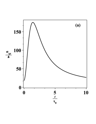
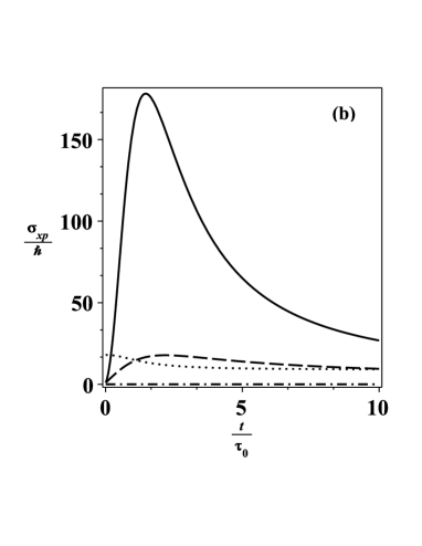
Figure 2: (a) Position-momentum correlations as a function of $t/\tau_{0}$ for $\tau=18\tau_{0}$. (b) Absolute value of the first (pointed line), second (solid line), third (dashed line) and fourth (dashed-point line) term of the equation (16) as a function of $t/\tau_{0}$ for $\tau=18\tau_{0}$. We observe a point of maximum and that the larger contribution to the correlations comes from the second term (solid line) of equation (16).

In Fig. 3, we show the position-momentum correlations as a function of $t/\tau_{0}$ and $\tau/\tau_{0}$. We observe that the region around the point of maximum, or region of phase instability, tends to stay narrower when the propagation time from the double-slit to the screen $\tau$ increases. We also observe that the point of maximum is displaced from the left when $\tau$ increases. In the next section we will show a table in which we clearly see the dependence of the time for the maximum of the correlations $t_{max}$ with the value of $\tau$, i.e., $t_{max}=t_{max}(\tau)$. Therefore, the dynamics after the double-slit also influences the interference pattern and should be taken into account in the analysis of double-slit experiments. Taking into account only the dynamics before the double-slit is not sufficient to obtain all the information about the interference pattern on the screen.

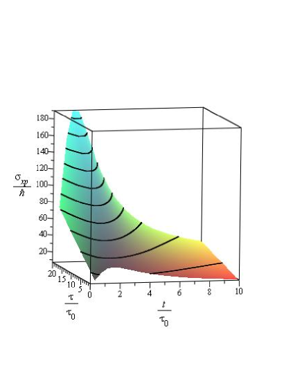
Figure 3: Position-momentum correlation as a function of $t/\tau_{0}$ and $\tau/\tau_{0}$. The maximum is displaced to the left and the region around it tends to stay more narrow when $\tau$ increases.

IV Schrodinger Uncertainty Relation

It is known that the uncorrelated free particle Gaussian wavepackets are states of minimum uncertainty both in position and in momentum. For this case the position-momentum correlations appear only with the time evolution and are followed by a spreading of the associated position distribution, while the momentum uncertainty is maintained constant for all time. For the most general Gaussian wavepacket, in which the initial position-momentum correlations are present, the uncertainty in position is minimum at $t=0$ but this is not true for the uncertainty in momentum Riahi . Therefore, the position-momentum correlations indicate that the uncertainty in one or in both the quadratures is not a minimum. For the problem treated here we have a superposition of two Gaussian wavepackets at the screen, for which the position-momentum correlations are present indicating that the uncertainty in both the quadratures is not minimum. To study the behavior of the correlations together with the behavior of the uncertainties in position and in momentum, we calculate in this section the determinant of the covariance matrix defined by

$$M_{C}=\left(\begin{array}[]{cc}\sigma_{xx}^{2}&\sigma_{xp}\\ \sigma_{xp}&\sigma_{pp}^{2}\end{array}\right),$$ (17)

where $\sigma_{xx}^{2}=\langle\hat{x}^{2}\rangle-\langle\hat{x}\rangle^{2}$, $\sigma_{pp}^{2}=\langle\hat{p}^{2}\rangle-\langle\hat{p}\rangle^{2}$ are the squared variances in position and momentum, respectively, and $\sigma_{xp}$ is the position-momentum correlations. The expression for $\sigma_{xp}$ was obtained previously in equation (16) and for the other quantities we obtain the following results

$$\sigma^{2}_{xx}(t,\tau)=\frac{B^{2}}{2}+\frac{D^{2}-4\Delta^{2}B^{4}\exp\left[-\left(\frac{D}{2B}\right)^{2}-\left(\Delta B\right)^{2}\right]}{4+4\exp\left[-\left(\frac{D}{2B}\right)^{2}-\left(\Delta B\right)^{2}\right]},$$ (18)

and

$$\frac{\sigma^{2}_{pp}(t,\tau)}{\hbar^{2}} = \left(\frac{1}{2B^{2}}+\frac{m^{2}B^{2}}{2\hbar^{2}R^{2}}\right)+\frac{\left(\frac{mD}{\hbar R}-2\Delta\right)^{2}}{4+4\exp\left[-\left(\frac{D}{2B}\right)^{2}-\left(\Delta B\right)^{2}\right]}$$ (19)

$$- \frac{\left[\frac{D^{2}}{B^{4}}+2\Delta\left(\Delta+\frac{mD}{\hbar R}\right)\right]}{1+\exp\left[\left(\frac{D}{2B}\right)^{2}+\left(\Delta B\right)^{2}\right]}.$$

The determinant of the covariance matrix, equation (17), is the generalized Robertson-Schrödinger uncertainty relation and it is given by

$$D_{C}=\sigma_{xx}^{2}\sigma_{pp}^{2}-\sigma_{xp}^{2}.$$ (20)

In Fig. 4a we show the curves of the uncertainties $\sigma_{xx}$, $\sigma_{pp}$ and the correlations $\sigma_{xp}$ normalized to the same scale as a function of $t/\tau_{0}$ for $\tau=18\tau_{0}$ and in Fig. 4b we show the determinant $D_{C}/\hbar^{2}$ (solid line) as a function of $t/\tau_{0}$ for $\tau=18\tau_{0}$, where we compared it with the value $1/4$ (dashed line). As the position-momentum correlations mean that both uncertainties are not minima, we see that this behavior is manifested in the determinant as a fast increasing in the region around the maximum of the correlations. The point of maximum is located between the maxima of the uncertainties in position and in momentum, and the region in which we can consider the correlations as maximum cover the interval $0.53\tau_{0}<t<4\tau_{0}$, where $t=0.52\tau_{0}$ is the inflexion point of the curve of $\sigma_{xp}$ and the other extreme $t\approx 4\tau_{0}$ corresponds to the point for which the correlations have the same value when $t=0.52\tau_{0}$, i.e., $\sigma_{xp}(t=0.52\tau_{0})\approx\sigma_{xp}(t=4\tau_{0})\approx 82\hbar$. On the other hand, the determinant varies slowly in the regions where the correlations tend to be minima, more specifically the regions $0<t<0.52\tau_{0}$ and $t>4\tau_{0}$. At the interval $0<t<0.52\tau_{0}$ the uncertainty in position and in momentum increases practically by the same rate and at the interval $t>4\tau_{0}$ the uncertainty in position decreases more slowly than the uncertainty in momentum. The determinant tends to a constant value in both intervals, but at the first interval, $0<t<0.52\tau_{0}$, the curve of correlations has a concavity upwards in which the value of the determinant tends to the minimum value $D_{C}\approx 16\hbar^{2}$. At the second interval, $t>4\tau_{0}$, the curve of correlations has a concavity turned down (tending to a constant function for $t\gg t_{max}$) in which the determinant tends to the maximum value $D_{C}\approx 33\hbar^{2}$. Then, we observe that $D_{C}>\hbar^{2}/4$ for all time. This characterizes the non-gaussianity of the state (15), since for Gaussian states, initially correlated or not, the generalized Robertson-Schrödinger uncertainty relation is constant and equal to $\hbar^{2}/4$ for all time. Therefore, for states obtained from the superposition of two Gaussian states, as the case treated here, the determinant of the covariance matrix is larger than $\hbar^{2}/4$ for all time and it is practically constant only for values of time outside the region around which the correlations have a point of maximum, showing that the Gaussian features are strictly altered by the evolution of the position-momentum correlations. Thus, if we construct one state that has correlations with a point of minimum, for which the determinant can tend to the value $\hbar^{2}/4$ at the screen, the number of interference fringes and its visibility can be increased significantly. It is possible to do this by considering one double-slit experiment in which the initial state is the correlated Gaussian state or by putting a atomic convergent lens next to the double-slit as similarly has been proposed for light waves Bartell .

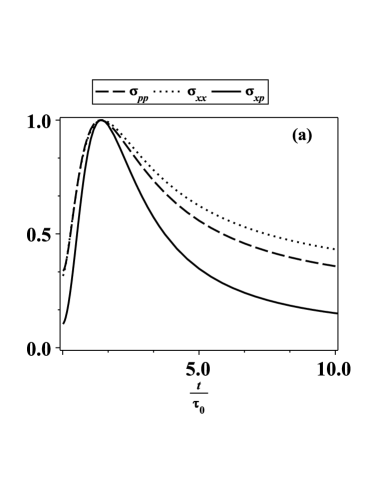
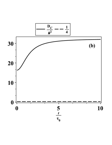
Figure 4: (a) Curves of the uncertainties $\sigma_{xx}$, $\sigma_{pp}$ and the correlations $\sigma_{xp}$ at the same scale as a function of $t/\tau_{0}$ for $\tau=18\tau_{0}$. (b) Determinant $D_{C}/\hbar^{2}$ (solid line) as a function of $t/\tau_{0}$ for $\tau=18\tau_{0}$ compared with the value $1/4$ (dashed line). The determinant is practically constant at the extremes but different from the value $\hbar^{2}/4$ and varies rapidly in the region where the position-momentum correlations have a maximum.

In table I we show some values of time $t_{max}$ that we calculate numerically, for which the correlations $\sigma_{xp}$, the uncertainty in position $\sigma_{xx}$ and the uncertainty in momentum $\sigma_{pp}$ are maxima and the point of inflexion of the correlations as a function of time $\tau$. We observe that when $\tau$ increases, the time $t_{max}$ of the correlations is dislocated to the left and that this time is always localized between the times for which the uncertainties in position and in momentum are maxima. We also observe that the times of maxima tend to coincide for $\tau>1000\tau_{0}$ and that the time of maximum for $\sigma_{pp}$ is independent of $\tau$ as a consequence of the free propagation from the double-slit to the screen.

Table 1: Times of maxima $t_{max}$ and inflexion $t_{inf}$ as a function of $\tau$. All terms in units of $\tau_{0}$

$\tau$	$t_{max}$ of $\sigma_{xp}$	$t_{max}$ of $\sigma_{xx}$	$t_{max}$ of $\sigma_{pp}$	$t_{inf}$ of $\sigma_{xp}$
2	1.568109061	1.984545314	1.392356020	0.4720349103
8	1.450312552	1.525841616	1.392356020	0.4990240822
18	1.419651602	1.450522331	1.392356020	0.5049187153
50	1.402487095	1.413088513	1.392356020	0.5080737518
100	1.397465783	1.402693625	1.392356020	0.5089789150
1000	1.392871030	1.393387225	1.392356020	0.5098004574

V Intensity, Visibility and Predictability

In this section we calculate the relative intensity, visibility and predictability to analyze the interference pattern, the wave-like and particle-like behavior from the knowledge of the position-momentum correlations. Such analysis is very important because it allows us to choose the set of parameters that provides the better interference pattern in the double-slit experiment. The knowledge of the correlations tells us if the particle sent by the source will behave more as wave-like or particle-like on the screen. In other words, if the particle is sent by one position for which the time of flight until the double-slit pertains to the interval around the maximum of the correlations, it will behave most as a particle for most values of $x$, excluding only the values near $x=0$.

The intensity on the screen, defined as $I(x,t,\tau)=|\psi(x,t,\tau)|^{2}$, is given by

$$I(x,t,\tau)=F(x,t,\tau)\left[1+\frac{\cos(2\Delta x)}{\cosh(\frac{Dx}{B^{2}})}\right],$$ (21)

where

$$F(x,t,\tau)=I_{0}\exp\left[-\frac{x^{2}+(\frac{D}{2})^{2}}{B^{2}}\right]\cosh\left(\frac{Dx}{B^{2}}\right).$$ (22)

The visibility and predictability are given, respectively, by

$$\mathcal{V}=\frac{I_{max}-I_{min}}{I_{max}+I_{min}}=\frac{1}{\cosh(\frac{Dx}{B^{2}})},$$ (23)

and

$$\mathcal{P}=\left|\frac{|\psi_{1}|^{2}-|\psi_{2}|^{2}}{|\psi_{1}|^{2}+|\psi_{2}|^{2}}\right|=\left|\tanh\left(\frac{Dx}{B^{2}}\right)\right|.$$ (24)

The Bohr’s complementarity principle established, by the relation of Greenberger and Yasin for pure quantum mechanical states, that $\mathcal{P}^{2}+\mathcal{V}^{2}=1$ is satisfied for all values of $x$ Greenberger . The visibility and predictability depend on the ratio $D/B^{2}$, showing the influence of the parameter $D$ (the separation between the wavepackets at the time), equivalently the position-momentum correlations, on the interference pattern. Therefore, for higher values of $D$ and smaller values of $B$, the particle-like behavior will be dominant and less visible will be the interference fringes. As we will see, there is a value of time $t$, within the interval of maximum correlations, for which the visibility is minimum and the predictability is maximum. Previously, the effective number of fringes for light waves in the double-slit was characterized in Ref. Bramon for a given distance (or time) of propagation from the double-slit to the screen while neglecting the propagation from the source to the double-slit. According to Bramon , the number of fringes was estimated by a new index defined by $\nu=0.264/\mathcal{R}$. For the problem treated here, we have $\mathcal{R}=D/2\Delta B^{2}$, indicating that the higher the value of $D$ is, the lesser the number of fringes is.

In Fig. 5a, we show the half of the symmetrical plot for the relative intensity (black line) and in Fig. 5b we show the half of the symmetrical plot of the visibility (blue line) and predictability (red line) as a function of $x$ for three different values of $t$, one of them being the time for which the correlations have a maximum, with $\tau$ fixed to $\tau=18\tau_{0}$. The corresponding values of $t$ are, respectively, $t=0.2\tau_{0}$ (solid line), $t_{max}\approx 1.42\tau_{0}$ (dotted line) and $t=18\tau_{0}$ (dashed line). We observe that for $t_{max}\approx 1.42\tau_{0}$ the number of interference fringes is a minimum and the visibility extends over a small range of the $x$ axis behind the double-slit. In addition, the predictability dominates extending over a wide range of the $x$ axis. For $t=0.2\tau_{0}$ or $t=18\tau_{0}$ we have a large number of fringes and the visibility extends over a larger range of the $x$ axis behind the double-slit. The predictability dominates only in a range outside the region immediately behind the double-slit. This shows that a displacement of the source either to the left or to the right, so that the particles flights a different time from the times around which the correlations have a maximum $t_{max}$, most specifically the times in the interval $0.52\tau_{0}<t<4\tau_{0}$, the number of fringes increases and the interference pattern presents a better quality. We have to focus on the region for which the correlations have a maximum and not specifically at the time of maximum since although $t_{max}$ really appears as the time for which the number of fringes is a minimum, the visibility has a minimum in the region of maximum correlations but it does not coincide with $t_{max}$ being displaced a little from this point to the right, as we can see in Fig. 6. In fact, for $t=0.2\tau_{0}$ and $t=18\tau_{0}$ the position-momentum correlations assume values close to each other, the number of fringes is nearly the same. However, the visibility is larger for $t=0.2\tau_{0}$, suggesting that the wave-like behavior will be most evident when the particle is released closer to the double-slit. Saying in a different way, our ignorance about which slit the particle passed increases when the particle is released closer to the double-slit. Therefore, although the complementarity relation $\mathcal{P}^{2}+\mathcal{V}^{2}=1$ is valid for all $x$ independent of the time (or distance) of propagation, the quantities $\mathcal{P}(x,t,\tau)$ and $\mathcal{V}(x,t,\tau)$ are substantially altered at each point $x$ by the propagation times $t$ and $\tau$, as quantitatively shown in Fig. 6.

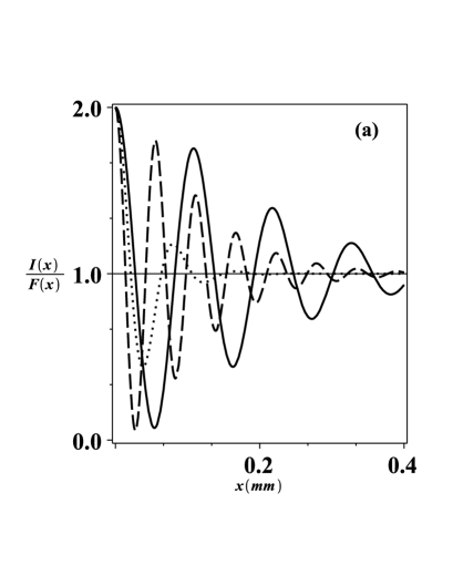
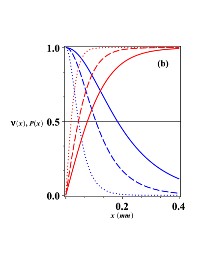
Figure 5: (a) Relative intensity (black line) and (b) visibility (blue line) and predictability (red line) as a function of $x$ for three different values of $t$ and $\tau=18\tau_{0}$. The corresponding values of $t$ are, respectively, $t=0.2\tau_{0}$ (solid line), $t_{max}\approx 1.42\tau_{0}$ (dotted line) and $t=18\tau_{0}$ (dashed line). For these values of time, the time for which the correlations have a maximum $t_{max}\approx 1.42\tau_{0}$ presents the least number of fringes and visibility. Moving the source of particles to the left or to the right from the region around the maximum of the correlations, the number of fringes and visibility increase.

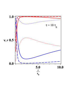
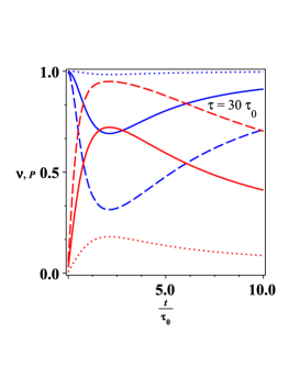
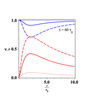
Figure 6: Visibility (blue line) and predictability (red line) as a function of $t/\tau_{0}$ for three different values of $x$. The corresponding values of $x$ are $x=0.01\;\mathrm{mm}$ (dotted line), $x=0.05\;\mathrm{mm}$ (solid line) and $x=0.1\;\mathrm{mm}$ (dashed line). We present figures for $\tau=10\tau_{0}$, $\tau=30\tau_{0}$ and $\tau=60\tau_{0}$. The values of $\mathcal{V}$ and $\mathcal{P}$ for each value of $x$ are strongly altered by the values of $t$ and $\tau$. For example, exist a value of time $t$ for which the visibility is minimum and the predictability is maximum and for $\tau>60\tau_{0}$ the values of $\mathcal{V}$ are higher than the values of $\mathcal{P}$.

In Fig. 7a, we show the half of the symmetrical plot for relative intensity (black line) and in Fig. 7b we show the half of the symmetrical plot of the visibility (blue line) and predictability (red line) as a function of $x$ for two different values of $\tau$, fixing $t$ at $t=8\tau_{0}$. The corresponding values of $\tau$ are, respectively, $\tau=10\tau_{0}$ (dashed line) and $\tau=30\tau_{0}$ (solid line). For $\tau=30\tau_{0}$, we have a larger number of fringes with a better visibility because the region of maximum correlations will be further for $t=8\tau_{0}$ with $\tau=30\tau_{0}$ than the $\tau=10\tau_{0}$ case, according to table I. In this case we observe that the displacement of the maximum of the correlations implies an increasing in the spatial transverse coherence with time. In fact, the number of interference fringes is nearly the same for both values of $\tau$, but the visibility is larger for $\tau=30\tau_{0}$ in comparison with $\tau=10\tau_{0}$. This shows that the wave-like behavior becomes more evident, comparatively, when the particle is launched from a position such that the flight time until the double-slit is most distant from the time for which the correlations have a maximum. On the other hand, we can say that our ignorance about which slit the particle passed, when it is launched from the position $z=v_{z}(t=8\tau_{0})$, is smaller when the screen is positioned at $z_{1}=v_{z}(\tau_{1}=10\tau_{0})$ than the situation where the screen is positioned at $z_{2}=v_{z}(\tau_{2}=30\tau_{0})$. Again, we see the influence of the times $t$ and $\tau$ over the quantities $\mathcal{P}(x,t,\tau)$ and $\mathcal{V}(x,t,\tau)$, although the result $\mathcal{P}^{2}+\mathcal{V}^{2}=1$ is maintained for all $x$ values independent of the time.

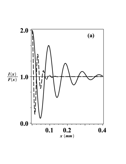
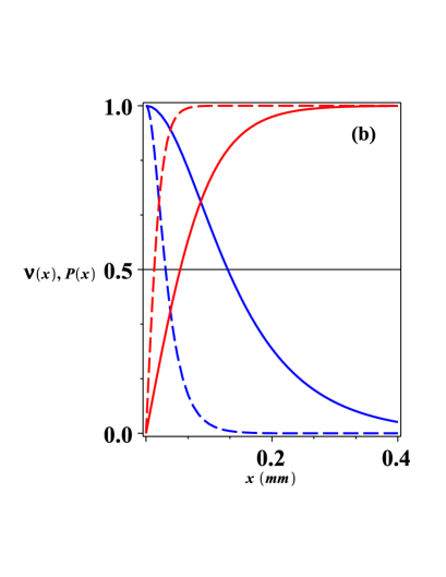
Figure 7: (a) Relative intensity (black line) and (b) visibility (blue line) and predictability (red line) as a function of $x$ for two different values of $\tau$ and $t$ fixed in $t=8\tau_{0}$. The corresponding values of $\tau$ are, respectively, $\tau=10\tau_{0}$ (dashed line) and $\tau=30\tau_{0}$ (solid line). For $\tau=30\tau_{0}$, we have the most number of interference fringes with a better visibility because the point for which the correlations have a maximum is more distant of $t=8\tau_{0}$ for $\tau=30\tau_{0}$, according to table I. In fact, the number of fringes is practically the same but the visibility is considerably larger for $\tau=30\tau_{0}$.

The results above were obtained for neutrons treated as wavepackets of initial transverse width $\sigma_{0}=7.8\;\mathrm{\mu m}$. For these parameters, the time scale is given by $\tau_{0}=m\sigma_{0}^{2}/\hbar=1.02\;\mathrm{ms}$. We can note a good quality in the interference pattern for $t=18\tau_{0}=18.02\;\mathrm{ms}$ and $\tau=18\tau_{0}=18.02\;\mathrm{ms}$, whose velocity around $v=200\;\mathrm{m/s}$, corresponds to distances $z_{t}=3.6\;\mathrm{m}$ and $z_{\tau}=3.6\;\mathrm{m}$. These parameters were used by A. Zeilinger et al. and they correspond to distances within the experimental viability Zeilinger1 . Now, if we take, for instance, the mass of the order of $m=1.2\times 10^{-24}\;\mathrm{kg}$, which is next to the mass of the fullerene molecules, and build a package of the same width of the neutrons, we will have $\tau_{0}=0.73\;\mathrm{s}$. In this case, $t=18\tau_{0}=13.14\;\mathrm{s}$ and $\tau=18\tau_{0}=13.14\;\mathrm{s}$. Considering one velocity of $200\;\mathrm{m/s}$, we will have $z_{t}=2.63\times 10^{3}\;\mathrm{m}$ and $z_{\tau}=2.63\times 10^{3}\;\mathrm{m}$, which are distances outside the experimental reality. Therefore, by analyzing the behavior of the correlations, we can also capture information about the difficulty in observing interference with macroscopic objects.

In Ref. Carol the authors explore the effect of the position-momentum correlations on the interference pattern but they do not take into account the influence of the propagation time from the double-slit to the screen. They also do not discuss the behavior of the correlations as a function of the propagation time from the source to the double-slit (or equivalently, the behavior of the correlations as a function of the parameter $\sigma_{0}$). We observe that for the parameters used in this reference, the correlations are maxima for $0.013\;\mathrm{\mu m}\leq\sigma_{0}\leq 0.02\;\mathrm{\mu m}$ and minima for $\sigma_{0}>1.0\;\mathrm{\mu m}$, which justify the poor interference pattern for $0.013\;\mathrm{\mu m}\leq\sigma_{0}\leq 0.02\;\mathrm{\mu m}$ and a rich interference pattern for $\sigma_{0}=6.0\;\mathrm{\mu m}$.

VI Conclusions

In this contribution, we studied the double-slit experiment as an attempt to find parameters that produce the maximum number of interference fringes and with the highest possible quality on the screen. Our results show that we can take information about the interference pattern by looking at the behavior of the position-momentum correlations, that are installed with the quantum dynamics. We observe that both the dynamics before and after the double-slit are important for the existence and quality of the interference fringes on the screen. Especially we observe that there is a value of propagation time from the source to the double-slit for which the correlations have a point of maximum, so that particles released by a source at the region around this point produce interference fringes on the screen with the worst quality. The wave-like and particle-like behavior expressed by the complementary relation of Greenberger and Yasin $\mathcal{P}^{2}+\mathcal{V}^{2}=1$ is also strongly influenced at each point $x$ by the times $t$ and $\tau$, i.e., depending where the particle came from and where the screen was positioned, it will behave most as a wave or most as a particle at the screen. The knowledge of the point of maximum of the position-momentum correlations can also help us to choose the best parameters which allow us to observe interference effects with macromolecules, such as fullerenes. From the determinant of the covariance matrix it was possible to observe how the Gaussian properties of the state produced on the screen by the superposition of two Gaussian are altered when the uncertainties in position and in momentum and the position-momentum correlations vary with the times $t$ and $\tau$.

References

- (1) R. Feynman, R. B. Leighton, M. L. Sands, The Feynman Lectures on Physics: Quantum Mechanics vol 3 (Reading, MA: Addison-Wesley, 1965), chapter 1.
- (2) N. Bohr, Nature 121 (1928) 580; W. K. Wootters, W. K. Zurek, Phys. Rev. D. 19 (1979) 473.
- (3) G. Möllentedt, C. Jönsson, Z. Phys. 155 (1959) 472.
- (4) A. Zeilinger, R. Gähler, C. G. Shull, W. Treimer, W. Mampe, Rev. Mod. Phys. 60 (1988) 1067.
- (5) O. Carnal, J. Mlynek, Phys. Rev. Lett. 66 (1991) 2689.
- (6) W. Schöllkopf, J. P. Toennies, Science 266 (1994) 1345.
- (7) M. Arndt et al., Nature 401 (1999) 680; O. Nairz, M. Arndt, A. Zeilinger, J. Mod. Opt. 47 (2000) 2811; O. Nairz, M. Arndt, A. Zeilinger, Am. J. Phys. 71 (2003) 319.
- (8) D. Bohm, Quantum Theory (Prentice-Hall, Englewood Cliffs, 1963), pp 200-205.
- (9) D. S. Saxon, Elementary Quantum Mechanics (McGraw-Hill, New York, 1968), pp. 62-66.
- (10) R. W. Robinett, M. A. Docheski, L. C. Bassett, Found. Of Phys. Lett. 18 (2005) 455.
- (11) N. Riahi, Eur. J. Phys. 34 (2013) 461.
- (12) V. V. Dodonov, J. Opt. B 4 (2002) R1; V. V. Dodonov, A. V. Dodonov, J. Russ. Laser Res. 35 (2014) 39.
- (13) R. A. Campos, J. Mod. Opt. 46 (1999) 1277.
- (14) G. Glionna et al, Physica A 387 (2008) 1485.
- (15) I. G. da Paz, M. C. Nemes, S. Pádua, C. H. Monken, J. G. Peixoto de Faria, Phys. Lett. A 374 (2010) 1660.
- (16) I. G. da Paz, P. L. Saldanha, M. C. Nemes, J. G. Peixoto de Faria, New Journal of Phys. 13 (2011) 125005.
- (17) A. Hansen, J. T. Schultz, N. P. Bigelow, Conference on Coherence and Quantum Optics Rochester, New York, United States, June 17-20, 2013.
- (18) G. Guzzinati, P. Schattschneider, K. Y. Bliokh, F. Nori, Jo Verbeeck, Phys. Rev. Lett. 110 (2013) 093601.
- (19) T. C. Petersen, D. M. Paganin, M. Weyland, T. P. Simula, S. A. Eastwood, M. J. Morgan, Phys. Rev. A 88 (2013) 043803.
- (20) H. J. Kull, New Journal of Phys. 14 (2012) 055013.
- (21) L. S. Bartell, Phys. Rev. D 21 (1980) 1698.
- (22) D. M. Greenberger, A. Yasin, Phys. Lett. A 128 (1988) 391.
- (23) A. Bramon, G. Garbarino, B. C. Hiesmayr, Phys. Rev. A 69 (2004) 022112.