Abstract

The second-order differential equation for a damped harmonic oscillator can be converted to two coupled first-order equations, with two two-by-two matrices leading to the group $Sp(2)$. It is shown that this oscillator system contains the essential features of Wigner’s little groups dictating the internal space-time symmetries of particles in the Lorentz-covariant world. The little groups are the subgroups of the Lorentz group whose transformations leave the four-momentum of a given particle invariant. It is shown that the damping modes of the oscillator correspond to the little groups for massive and imaginary-mass particles respectively. When the system makes the transition from the oscillation to damping mode, it corresponds to the little group for massless particles. Rotations around the momentum leave the four-momentum invariant. This degree of freedom extends the $Sp(2)$ symmetry to that of $SL(2,c)$ corresponding to the Lorentz group applicable to the four-dimensional Minkowski space. The Poincaré sphere contains the $SL(2,c)$ symmetry. In addition, it has a non-Lorentzian parameter allowing us to reduce the mass continuously to zero. It is thus possible to construct the little group for massless particles from that of the massive particle by reducing its mass to zero. Spin-1/2 particles and spin-1 particles are discussed in detail.

1 Introduction

We are quite familiar with the second-order differential equation

$$m\frac{d^{2}y}{dt^{2}}+b\frac{dy}{dt}+Ky=0,$$ (1)

for a damped harmonic oscillator. This equation has the same mathematical form as

$$L\frac{d^{2}Q}{dt^{2}}+R\frac{dQ}{dt}+\frac{1}{C}Q=0,$$ (2)

for electrical circuits, where $L,R,$ and $C$ are the inductance, resistance, and capacitance respectively. These two equations play fundamental roles in physical and engineering sciences. Since they start from the same set of mathematical equations, one set of problems can be studied in terms of the other. For instance, many mechanical phenomena can be studied in terms of electrical circuits.

In Eq.(1), when $b=0$, the equation is that of a simple harmonic oscillator with the frequency $\omega=\sqrt{K/m}$. As $b$ increases, the oscillation becomes damped. When $b$ is larger than $2\sqrt{Km}$, the oscillation disappears, as the solution is a damping mode.

Consider that increasing $b$ continuously, while difficult mechanically, can be done electrically using Eq.(2) by adjusting the resistance $R.$ The transition from the oscillation mode to the damping mode is a continuous physical process.

This $b$ term leads to energy dissipation, but is not regarded as a fundamental force. It is inconvenient in the Hamiltonian formulation of mechanics and troublesome in transition to quantum mechanics, yet, plays an important role in classical mechanics. In this paper this term will help us understand the fundamental space-time symmetries of elementary particles.

We are interested in constructing the fundamental symmetry group for particles in the Lorentz-covariant world. For this purpose, we transform the second-order differential equation of Eq.(1) to two coupled first-order equations using two-by-two matrices. Only two linearly independent matrices are needed. They are the anti-symmetric and symmetric matrices

$$A=\pmatrix{0&-i\cr i&0},\quad\mbox{and}\quad S=\pmatrix{0&i\cr i&0},$$ (3)

respectively. The anti-symmetric matrix $A$ is Hermitian and corresponds to the oscillation part, while the symmetric $S$ matrix corresponds to the damping.

These two matrices lead to the $Sp(2)$ group consisting of two-by-two unimodular matrices with real elements. This group is isomorphic to the three-dimensional Lorentz group applicable to two space-like and one time-like coordinates. This group is commonly called the $O(2,1)$ group.

This $O(2,1)$ group can explain all the essential features of Wigner’s little groups dictating internal space-time symmetries of particles [1]. Wigner defined his little groups as the subgroups of the Lorentz group whose transformations leave the four-momentum of a given particle invariant. He observed that the little groups are different for massive, massless, and imaginary-mass particles. It has been a challenge to design a mathematical model which will combine those three into one formalism, but we show that the damped harmonic oscillator provides the desired mathematical framework.

For the two space-like coordinates, we can assign one of them to the direction of the momentum, and the other to the direction perpendicular to the momentum. Let the direction of the momentum be along the $z$ axis, and let the perpendicular direction be along the $x$ axis. We therefore study the kinematics of the group within the $zx$ plane, then see what happens when we rotate the system around the $z$ axis without changing the momentum [2].

The Poincaré sphere for polarization optics contains the $SL(2,c)$ symmetry isomorphic to the four-dimensional Lorentz group applicable to the Minkowski space [3, 4, 5, 6, 7]. Thus, the Poincaré sphere extends Wigner’s picture into the three space-like and one time-like coordinates. Specifically, this extension adds rotations around the given momentum which leaves the four-momentum invariant [2].

While the particle mass is a Lorentz-invariant variable, the Poincaré sphere contains an extra variable which allows the mass to change. This variable allows us to take the mass-limit of the symmetry operations. The transverse rotational degrees of freedom collapse into one gauge degree of freedom and polarization of neutrinos is a consequence of the requirement of gauge invariance [8, 9].

The $SL(2,c)$ group contains symmetries not seen in the three-dimensional rotation group. While we are familiar with two spinors for a spin-1/2 particle in nonrelativistic quantum mechanics, there are two additional spinors due to the reflection properties of the Lorentz group. There are thus sixteen bilinear combinations of those four spinors. This leads to two scalars, two four-vectors, and one antisymmetric four-by-four tensor. The Maxwell-type electromagnetic field tensor can be obtained as a massless limit of this tensor [10].

In Sec. 2, we review the damped harmonic oscillator in classical mechanics, and note that the solution can be either in the oscillation mode or damping mode depending on the magnitude of the damping parameter. The translation of the second order equation into a first order differential equation with two-by-two matrices is possible. This first-order equation is similar to the Schrödinger equation for a spin-1/2 particle in a magnetic field.

Section 3 shows that the two-by-two matrices of Sec. 2 can be formulated in terms of the $Sp(2)$ group. These matrices can be decomposed into the Bargmann and Wigner decompositions. Furthermore, this group is isomorphic to the three-dimensional Lorentz group with two space and one time-like coordinates.

In Sec. 4, it is noted that this three-dimensional Lorentz group has all the essential features of Wigner’s little groups which dictate the internal space-time symmetries of the particles in the Lorentz-covariant world. Wigner’s little groups are the subgroups of the Lorentz group whose transformations leave the four-momentum of a given particle invariant. The Bargmann Wigner decompositions are shown to be useful tools for studying the little groups.

In Sec. 5, we note that the given momentum is invariant under rotations around it. The addition of this rotational degree of freedom extends the $Sp(2)$ symmetry to the six-parameter $SL(2,c)$ symmetry. In the space-time language, this extends the three dimensional group to the Lorentz group applicable to three space and one time dimensions.

Section 6 shows that the Poincaré sphere contains the symmetries of $SL(2,c)$ group. In addition, it contains an extra variable which allows us to change the mass of the particle, which is not allowed in the Lorentz group.

In Sec. 7, the symmetries of massless particles are studied in detail. In addition to rotation around the momentum, Wigner’s little group generates gauge transformations. While gauge transformations on spin-1 photons are well known, the gauge invariance leads to the polarization of massless spin-1/2 particles, as observed in neutrino polarizations.

In Sec. 8, it is noted that there are four spinors for spin-1/2 particles in the Lorentz-covariant world. It is thus possible to construct sixteen bilinear forms, applicable to two scalars, and two vectors, and one antisymmetric second-rank tensor. The electromagnetic field tensor is derived as the massless limit. This tensor is shown to be gauge-invariant.

2 Classical Damped Oscillators

For convenience, we write Eq.(1) as

$$\frac{d^{2}y}{dt^{2}}+2\mu\frac{dy}{dt}+\omega^{2}y=0,$$ (4)

with

$$\omega=\sqrt{\frac{K}{m}},\quad\mbox{and}\quad\mu=\frac{b}{2m},$$ (5)

The damping parameter $\mu$ is positive when there are no external forces. When $\omega$ is greater than $\mu$, the solution takes the form

$$y=e^{-\mu t}\left[C_{1}\cos(\omega^{\prime}t)+C_{2}\sin(\omega^{\prime}t)\right],$$ (6)

where

$$\omega^{\prime}=\sqrt{\omega^{2}-\mu^{2}},$$ (7)

and $C_{1}$ and $C_{2}$ are the constants to be determined by the initial conditions. This expression is for a damped harmonic oscillator. Conversely, when $\mu$ is greater than $\omega$, the quantity inside the square-root sign is negative, then the solution becomes

$$y=e^{-\mu t}\left[C_{3}\cosh(\mu^{\prime}t)+C_{4}\sinh(\mu^{\prime}t)\right],$$ (8)

with

$$\mu^{\prime}=\sqrt{\mu^{2}-\omega^{2}},$$ (9)

If $\omega=\mu$, both Eq.(6) and Eq.(8) collapse into one solution

$$y(t)=e^{-\mu t}\left[C_{5}+C_{6}~{}t\right].$$ (10)

These three different cases are treated separately in textbooks. Here we are interested in the transition from Eq.(6) to Eq.(8), via Eq.(10). For convenience, we start from $\mu$ greater than $\omega$ with $\mu^{\prime}$ given by Eq.(9).

For a given value of $\mu$, the square root becomes zero when $\omega$ equals $\mu$. If $\omega$ becomes larger, the square root becomes imaginary and divides into two branches.

$$\pm i\sqrt{\omega^{2}-\mu^{2}}.$$ (11)

This is a continuous transition, but not an analytic continuation. To study this in detail, we translate the second order differential equation of Eq.(4) into the first-order equation with two-by-two matrices.

Given the solutions of Eq.(6), and Eq.(10), it is convenient to use $\psi(t)$ defined as

$$\psi(t)=e^{\mu t}y(t),\quad\mbox{and}\quad\quad y=e^{-\mu t}\psi(t).$$ (12)

Then $\psi(t)$ satisfies the differential equation

$$\frac{d^{2}\psi(t)}{dt^{2}}+(\omega^{2}-\mu^{2})\psi(t)=0.$$ (13)

2.1 Two-by-two Matrix Formulation

In order to convert this second order equation to a first order system we introduce $\psi_{1,2}(t)=(\psi_{1}(t),\psi_{2}(t))$. Then we have a system of two equations

$$\frac{d\psi_{1}(t)}{dt}=(\mu-\omega)\psi_{2}(t),$$

$$\frac{d\psi_{2}(t)}{dt}=(\mu+\omega)\psi_{1}(t)$$ (14)

which can be written in matrix form as

$$\frac{d}{dt}\pmatrix{\psi_{1}\cr\psi_{2}}=\pmatrix{0&\mu-\omega\cr\mu+\omega&0}\pmatrix{\psi_{1}\cr\psi_{2}}.$$ (15)

Using the Hermitian and anti-Hermitian matrices of Eq.(3) in Sec. 1, we construct the linear combination

$$H=\omega\pmatrix{0&-i\cr i&0}+\mu\pmatrix{0&i\cr i&0}.$$ (16)

We can then consider the first-order differential equation

$$i\frac{\partial}{\partial t}\psi(t)=H\psi(t).$$ (17)

While this equation is like the Schrödinger equation for an electron in a magnetic field, the two-by-two matrix is not Hermitian. Its first matrix is Hermitian, but the second matrix is anti-Hermitian. It is of course an interesting problem to give a physical interpretation to this non-Hermitian matrix in connection with quantum dissipation [11], but this is beyond the scope of the present paper. The solution of Eq.(17) is

$$\psi(t)=\exp{\left\{\pmatrix{0&-\omega+\mu\cr\omega+\mu&0}t\right\}}\pmatrix{C_{7}\cr C_{8}},$$ (18)

where $C_{7}=\psi_{1}(0)$ and $C_{8}=\psi_{2}(0)$ respectively.

2.2 Transition from the Oscillation Mode to Damping Mode

It appears straight-forward to compute this expression by a Taylor expansion, but it is not. This issue was extensively discussed in previous papers by two of us [12, 13]. The key idea is to write the matrix

$$\pmatrix{0&-\omega+\mu\cr\omega+\mu&0}$$ (19)

as a similarity transformation of

$$\omega^{\prime}\pmatrix{0&-1\cr 1&0}\quad\quad(\omega>\mu),$$ (20)

and as that of

$$\mu^{\prime}\pmatrix{0&1\cr 1&0}\quad\quad(\mu>\omega),$$ (21)

with $\omega^{\prime}$ and $\mu^{\prime}$ defined in Eq.(7) and Eq.(9), respectively.

Then the Taylor expansion leads to

$$\pmatrix{\cos(\omega^{\prime}t)&-\sqrt{(\omega-\mu)/(\omega+\mu)}~{}\sin(\omega^{\prime}t)\cr\sqrt{(\omega+\mu)/(\omega-\mu)}~{}\sin(\omega^{\prime}t)&\cos(\omega^{\prime}t)},$$ (22)

when $\omega$ is greater than $\mu$. The solution $\psi(t)$ takes the form

$$\pmatrix{C_{7}\cos(\omega^{\prime}t)-C_{8}\sqrt{(\omega-\mu)/(\omega+\mu)}~{}\sin(\omega^{\prime}t)\cr C_{7}\sqrt{(\omega+\mu)/(\omega-\mu)}~{}\sin(\omega^{\prime}t)+C_{8}\cos(\omega^{\prime}t)}.$$ (23)

If $\mu$ is greater than $\omega$, the Taylor expansion becomes

$$\pmatrix{\cosh(\mu^{\prime}t)&\sqrt{(\mu-\omega)/(\mu+\omega)}~{}\sinh(\mu^{\prime}t)\cr\sqrt{(\mu+\omega)/(\mu-\omega)}~{}\sinh(\mu^{\prime}t)&\cosh(\mu^{\prime}t)}.$$ (24)

When $\omega$ is equal to $\mu$, both Eqs.(22) and (24) become

$$\pmatrix{1&0\cr 2\omega t&1}.$$ (25)

If $\omega$ is sufficiently close to but smaller than $\mu$, the matrix of Eq.(24) becomes

$$\pmatrix{1+(\epsilon/2)(2\omega t)^{2}&+\epsilon(2\omega t)\cr(2\omega t)&1+(\epsilon/2)(2\omega t)^{2}},$$ (26)

with

$$\epsilon=\frac{\mu-\omega}{\mu+\omega}.$$ (27)

If $\omega$ is sufficiently close to $\mu$, we can let

$$\mu+\omega=2\omega,\quad\mbox{and}\quad\mu-\omega=2\mu\epsilon.$$ (28)

If $\omega$ is greater than $\mu$, $\epsilon$ defined in Eq.(27) becomes negative, the matrix of Eq.(22) becomes

$$\pmatrix{1-(-\epsilon/2)(2\omega t)^{2}&-(-\epsilon)(2\omega t)\cr 2\omega t&1-(-\epsilon/2)(2\omega t)^{2}}.$$ (29)

We can rewrite this matrix as

$$\pmatrix{1-(1/2)\left[\left(2\omega\sqrt{-\epsilon}\right)t\right]^{2}&-\sqrt{-\epsilon}\left[\left(2\omega\sqrt{-\epsilon}\right)t\right]\cr 2\omega t&1-(1/2)\left[\left(2\omega\sqrt{-\epsilon}\right)t\right]^{2}}.$$ (30)

If $\epsilon$ becomes positive, Eq.(26) can be written as

$$\pmatrix{1+(1/2)\left[\left(2\omega\sqrt{\epsilon}\right)t\right]^{2}&\sqrt{\epsilon}\left[\left(2\omega\sqrt{\epsilon}\right)t\right]\cr 2\omega t&1+(1/2)\left[\left(2\omega\sqrt{\epsilon}\right)t\right]^{2}}.$$ (31)

The transition from Eq.(30) to Eq.(31) is continuous as they become identical when $\epsilon=0.$ As $\epsilon$ changes its sign, the diagonal elements of above matrices tell us how $\cos(\omega^{\prime}t)$ becomes $\cosh(\mu^{\prime}t)$. As for the upper-right element element, $-\sin(\omega^{\prime}t)$ becomes $\sinh(\mu^{\prime}t).$ This non-analytic continuity is illustrated in Fig. 1.

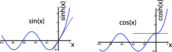
Figure 1: Transitions from $\sin$ to $\sinh$, and from $\cos$ to $\cosh.$ They are continuous transitions. Their first derivatives are also continuous, but the second derivatives are not. Thus, they are not analytically but only tangentially continuous.

2.3 Mathematical Forms of the Solutions

In this section, we use the Heisenberg approach to the problem, and obtain the solutions in the form of two-by-two matrices. We note that

• For the oscillation mode, the trace of the matrix is smaller than 2. The solution takes the form of

  $$\pmatrix{\cos(x)&-e^{-\eta}\sin(x)\cr e^{\eta}\sin(x)&\cos(x)},$$ (32)

  with trace $2\cos(x)$. The trace is independent of $\eta$.

• For the damping mode, the trace of the matrix is greater than 2.

  $$\pmatrix{\cosh(x)&e^{-\eta}\sinh(x)\cr e^{\eta}\sinh(x)&\cosh(x)},$$ (33)

  with trace $2\cosh(x)$. Again, the trace is independent of $\eta$.

• For the transition mode, the trace is equal to 2, and the matrix is triangular and takes the form of

  $$\pmatrix{1&0\cr\gamma&1}.$$ (34)

When $x$ approaches zero, the Eq.(32) and Eq.(33) take the form

$$\pmatrix{1-x^{2}/2&-xe^{-\eta}\cr xe^{\eta}&1-x^{2}/2},\quad\mbox{and}\quad\pmatrix{1+x^{2}/2&xe^{-\eta}\cr xe^{\eta}&1+x^{2}/2},$$ (35)

respectively. These two matrices have the same lower-left element. Let us fix this element to be a positive number $\gamma$. Then

$$x=\gamma e^{-\eta}.$$ (36)

Then the matrices of Eq.(35) become

$$\pmatrix{1-\gamma^{2}e^{-2\eta}/2&-\gamma e^{-2\eta}\cr\gamma&1-\gamma^{2}e^{-2\eta}/2},\quad\mbox{and}\quad\pmatrix{1+\gamma^{2}e^{-2\eta}/2&\gamma e^{-2\eta}\cr\gamma&1+\gamma^{2}e^{-2\eta}/2},$$ (37)

If we introduce a small number $\epsilon$ defined as

$$\epsilon=\sqrt{\gamma}e^{-\eta},$$ (38)

the matrices of Eq.(37) become

$$\begin{array}[]{cc}\pmatrix{e^{-\eta/2}&0\cr 0&e^{\eta/2}}\pmatrix{1-\gamma\epsilon^{2}/2&\sqrt{\gamma}\epsilon\cr\sqrt{\gamma}\epsilon&1-\gamma\epsilon^{2}/2}\pmatrix{e^{\eta/2}&0\cr 0&e^{-\eta/2}},\\ \\ \pmatrix{e^{-\eta/2}&0\cr 0&e^{\eta/2}}\pmatrix{1+\gamma\epsilon^{2}/2&\sqrt{\gamma}\epsilon\cr\sqrt{\gamma}\epsilon&1+\gamma\epsilon^{2}/2}\pmatrix{e^{\eta/2}&0\cr 0&e^{-\eta/2}}\end{array}$$ (39)

respectively, with $e^{-\eta}=\epsilon/\sqrt{\gamma}$.

3 Groups of Two-by-two Matrices

If a two-by-two matrix has four complex elements, it has eight independent parameters. If the determinant of this matrix is one, it is known as an unimodular matrix and the number of independent parameters is reduced to six. The group of two-by-two unimodular matrices is called $SL(2,c)$. This six-parameter group is isomorphic to the Lorentz group applicable to the Minkowski space of three space-like and one time-like dimensions [15].

We can start with two subgroups of $SL(2,c)$.

• While the matrices of $SL(2,c)$ are not unitary, we can consider the subset consisting of unitary matrices. This subgroup is called $SU(2)$, and is isomorphic to the three-dimensional rotation group. This three-parameter group is the basic scientific language for spin-1/2 particles.

• We can also consider the subset of matrices with real elements. This three-parameter group is called $Sp(2)$ and is isomorphic to the three-dimensional Lorentz group applicable to two space-like and one time-like coordinates.

In the Lorentz group, there are three space-like dimensions with $x,y,$ and $z$ coordinates. However, for many physical problems, it is more convenient to study the problem in the two-dimensional $(x,z)$ plane first and generalize it to three-dimensional space by rotating the system around the $z$ axis. This process can be called Euler decomposition and Euler generalization [2].

First we study $Sp(2)$ symmetry in detail, and achieve the generalization by augmenting the two-by-two matrix corresponding to the rotation around the $z$ axis. In this section, we study in detail properties of $Sp(2)$ matrices, then generalize them to $SL(2,c)$ in Sec. 5.

There are three classes of $Sp(2)$ matrices. Their traces can be smaller or greater than two, or equal to two. While these subjects are already discussed in the literature [16, 17, 18] our main interest is what happens as the trace goes from less than two to greater than two. Here we are guided by the model we have discussed in Sec. 2, which accounts for the transition from the oscillation mode to the damping mode.

3.1 Lie Algebra of Sp(2)

The two linearly independent matrices of Eq.(3) can be written as

$$K_{1}=\frac{1}{2}\pmatrix{0&i\cr i&0},\quad\mbox{and}\quad J_{2}=\frac{1}{2}\pmatrix{0&-i\cr i&0}.$$ (40)

However, the Taylor series expansion of the exponential form of Eq.(22) or Eq.(24) requires an additional matrix

$$K_{3}=\frac{1}{2}\pmatrix{i&0\cr 0&-i}.$$ (41)

These matrices satisfy the following closed set of commutation relations.

$$\left[K_{1},J_{2}\right]=iK_{3},\qquad\left[J_{2},K_{3}\right]=iK_{1},\qquad\left[K_{3},K_{1}\right]=-iJ_{2}.$$ (42)

These commutation relations remain invariant under Hermitian conjugation, even though $K_{1}$ and $K_{3}$ are anti-Hermitian. The algebra generated by these three matrices is known in the literature as the group $Sp(2)$ [18]. Furthermore, the closed set of commutation relations is commonly called the Lie algebra. Indeed, Eq.(42) is the Lie algebra of the $Sp(2)$ group.

The Hermitian matrix $J_{2}$ generates the rotation matrix

$$R(\theta)=\exp{\left(-i\theta J_{2}\right)}=\pmatrix{\cos(\theta/2)&-\sin(\theta/2)\cr\sin(\theta/2)&\cos(\theta/2)},$$ (43)

and the anti-Hermitian matrices $K_{1}$ and $K_{2}$, generate the following squeeze matrices.

$$S(\lambda)=\exp{\left(-i\lambda K_{1}\right)}=\pmatrix{\cosh(\lambda/2)&\sinh(\lambda/2)\cr\sinh(\lambda/2)&\cosh(\lambda/2)},$$ (44)

and

$$B(\eta)=\exp{\left(-i\eta K_{3}\right)}=\pmatrix{\exp{(\eta/2)}&0\cr 0&\exp{(-\eta/2)}},$$ (45)

respectively.

Returning to the Lie algebra of Eq.(42), since $K_{1}$ and $K_{3}$ are anti-Hermitian, and $J_{2}$ is Hermitian, the set of commutation relation is invariant under the Hermitian conjugation. In other words, the commutation relations remain invariant, even if we change the sign of $K_{1}$ and $K_{3}$, while keeping that of $J_{2}$ invariant. Next, let us take the complex conjugate of the entire system. Then both the $J$ and $K$ matrices change their signs.

3.2 Bargmann and Wigner Decompositions

Since the $Sp(2)$ matrix has three independent parameters, it can be written as [16]

$$\pmatrix{\cos\left(\alpha_{1}/2\right)&-\sin\left(\alpha_{1}/2\right)\cr\sin\left(\alpha_{1}/2\right)&\cos\left(\alpha_{1}/2\right)}\pmatrix{\cosh\chi&\sinh\chi\cr\sinh\chi&\cosh\chi}\pmatrix{\cos\left(\alpha_{2}/2\right)&-\sin\left(\alpha_{2}/2\right)\cr\sin\left(\alpha_{2}/2\right)&\cos\left(\alpha_{2}/2\right)}$$ (46)

This matrix can be written as

$$\pmatrix{\cos(\delta/2)&-\sin(\delta/2)\cr\sin(\delta/2)&\cos(\delta/2)}\pmatrix{a&b\cr c&d}\pmatrix{\cos(\delta/2)&\sin(\delta/2)\cr-\sin(\delta/2)&\cos(\delta/2)}$$ (47)

where

$$\pmatrix{a&b\cr c&d}=\pmatrix{\cos(\alpha/2)&-\sin(\alpha/2)\cr\sin(\alpha/2)&\cos(\alpha/2)}\pmatrix{\cosh\chi&\sinh\chi\cr\sinh\chi&\cosh\chi}\pmatrix{\cos(\alpha/2)&-\sin(\alpha/2)\cr\sin(\alpha/2)&\cos(\alpha/2)}$$ (48)

with

$$\delta=\frac{1}{2}\left(\alpha_{1}-\alpha_{2}\right),\quad\mbox{and}\quad\alpha=\frac{1}{2}\left(\alpha_{1}+\alpha_{2}\right).$$ (49)

If we complete the matrix multiplication of Eq.(48), the result is

$$\pmatrix{(\cosh\chi)\cos\alpha&\sinh\chi-(\cosh\chi)\sin\alpha\cr\sinh\chi+(\cosh\chi)\sin\alpha&(\cosh\chi)\cos\alpha}.$$ (50)

We shall call hereafter the decomposition of Eq.(48) the Bargmann decomposition. This means that every matrix in the $Sp(2)$ group can be brought to the Bargmann decomposition by a similarity transformation of rotation, as given in Eq.(47). This decomposition leads to an equidiagonal matrix with two independent parameters.

For the matrix of Eq.(48), we can now consider the following three cases. Let us assume that $\chi$ is positive, and the angle $\theta$ is less than $90^{o}$. Let us look at the upper-right element.

• If it is negative with $[\sinh\chi<(\cosh\chi)\sin\alpha]$, then the trace of the matrix is smaller than 2, and the matrix can be written as

  $$\pmatrix{\cos(\theta/2)&-e^{-\eta}\sin(\theta/2)\cr e^{\eta}\sin(\theta/2)&\cos(\theta/2)},$$ (51)

  with

  $$\cos(\theta/2)=(\cosh\chi)\cos\alpha,\quad\mbox{and}\quad e^{-2\eta}=\frac{(\cosh\chi)\sin\alpha-\sinh\chi}{(\cosh\chi)\sin\alpha+\sinh\chi}.$$ (52)

• If it is positive with $[\sinh\chi>(\cosh\chi)\sin\alpha)]$, then the trace is greater than 2, and the matrix can be written as

  $$\pmatrix{\cosh(\lambda/2)&e^{-\eta}\sinh(\lambda/2)\cr e^{\eta}\sinh(\lambda/2)&\cosh(\lambda/2)},$$ (53)

  with

  $$\cosh(\lambda/2)=(\cosh\chi)\cos\alpha,\quad\mbox{and}\quad e^{-2\eta}=\frac{\sinh\chi-(\cosh\chi)\sin\alpha}{(\cosh\chi)\sin\alpha+\sinh\chi}.$$ (54)

• If it is zero with $[(\sinh\chi=(\cosh\chi)\sin\alpha)]$, then the trace is equal to 2, and the matrix takes the form

  $$\pmatrix{1&0\cr 2\sinh\chi&1},$$ (55)

The above repeats the mathematics given in Subsec. 2.3.

Returning to Eq.(51) and Eq.(52), they can be decomposed into

$$M(\theta,\eta)=\pmatrix{e^{\eta/2}&0\cr 0&e^{-\eta/2}}\pmatrix{\cos(\theta/2)&-\sin(\theta/2)\cr\sin(\theta/2)&\cos(\theta/2)}\pmatrix{e^{-\eta/2}&0\cr 0&e^{\eta/2}},$$ (56)

and

$$M(\lambda,\eta)=\pmatrix{e^{\eta/2}&0\cr 0&e^{-\eta/2}}\pmatrix{\cosh(\lambda/2)&\sinh(\lambda/2)\cr\sinh(\lambda/2)&\cos(\lambda/2)}\pmatrix{e^{-\eta/2}&0\cr 0&e^{\eta/2}},$$ (57)

respectively. In view of the physical examples given in Sec. 7, we shall call this the “Wigner decomposition.” Unlike the Bargmann decomposition, the Wigner decomposition is in the form of a similarity transformation.

We note that both Eq.(56) and Eq.(57) are written as similarity transformations. Thus

$$[M(\theta,\eta)]^{n}=\pmatrix{\cos(n\theta/2)&-e^{-\eta}\sin(n\theta/2)\cr e^{\eta}\sin(n\theta/2)&\cos(n\theta/2)},$$ (58)

$$[M(\lambda,\eta)]^{n}=\pmatrix{\cosh(n\lambda/2)&e^{\eta}\sinh(n\lambda/2)\cr e^{-\eta}\sinh(n\lambda/2)&\cosh(n\lambda/2)},$$

$$[M(\gamma)]^{n}=\pmatrix{1&0\cr n\gamma&1}.$$

These expressions are useful for studying periodic systems [14].

The question is what physics these decompositions describe in the real world. To address this, we study what the Lorentz group does in the real world, and study isomorphism between the $Sp(2)$ group and the Lorentz group applicable to the three-dimensional space consisting of one time and two space coordinates.

3.3 Isomorphism with the Lorentz group

The purpose of this section is to give physical interpretations of the mathematical formulas given in Subsec. 3.2. We will interpret these formulae in terms of the Lorentz transformations which are normally described by four-by-four matrices. For this purpose, it is necessary to establish a correspondence between the two-by-two representation of Sec. 3.2 and the four-by-four representations of the Lorentz group.

Let us consider the Minkowskian space-time four-vector

$$(t,z,x,y)$$ (59)

where $\left(t^{2}-z^{2}-x^{2}-y^{2}\right)$ remains invariant under Lorentz transformations. The Lorentz group consists of four-by-four matrices performing Lorentz transformations in the Minkowski space.

In order to give physical interpretations to the three two-by-two matrices given in Eq.(43), Eq.(44), and Eq.(45), we consider rotations around the $y$ axis, boosts along the $x$ axis, and boosts along the $z$ axis. The transformation is restricted in the three-dimensional subspace of $(t,z,x)$. It is then straight-forward to construct those four-by-four transformation matrices where the $y$ coordinate remains invariant. They are given in Table 1. Their generators also given. Those four-by-four generators satisfy the Lie algebra given in Eq.( 42).

Table 1: Matrices in the two-by-two representation, and their corresponding four-by-four generators and transformation matrices.

	Matrices		Generators		Four-by-four		Transform Matrices
	$R(\theta)$		$J_{2}=\frac{1}{2}\pmatrix{0&-i\cr i&0}$		$\pmatrix{0&0&0&0\cr 0&0&-i&0\cr 0&i&0&0\cr 0&0&0&0}$		$\pmatrix{1&0&0&0\cr 0&\cos\theta&-\sin\theta&0\cr 0&\sin\theta&\cos\theta&0\cr 0&0&0&1}$
	$B(\eta)$		$K_{3}=\frac{1}{2}\pmatrix{i&0\cr 0&-i}$		$\pmatrix{0&i&0&0\cr i&0&0&0\cr 0&0&0&0\cr 0&0&0&0}$		$\pmatrix{\cosh\eta&\sinh\eta&0&0\cr\sinh\eta&\cosh\eta&0&0\cr 0&0&1&0\cr 0&0&0&1}$
	$S(\lambda)$		$K_{1}=\frac{1}{2}\pmatrix{0&i\cr i&0}$		$\pmatrix{0&0&i&0\cr 0&0&0&0\cr i&0&0&0\cr 0&0&0&0}$		$\pmatrix{\cosh\lambda&0&\sinh\lambda&0\cr 0&1&0&0\cr\sinh\lambda&0&\cosh\lambda&0\cr 0&0&0&1}$

4 Internal Space-time Symmetries

We have seen that there corresponds a two-by-two matrix for each four-by-four Lorentz transformation matrix. It is possible to give physical interpretations to those four-by-four matrices. It must thus be possible to attach a physical interpretation to each two-by-two matrix.

Since 1939 [1] when Wigner introduced the concept of the little groups many papers have been published on this subject, but most of them were based on the four-by-four representation. In this section, we shall give the formalism of little groups in the language of two-by-two matrices. In so doing, we provide physical interpretations to the Bargmann and Wigner decompositions introduced in Sec. 3.2.

4.1 Wigner’s Little Groups

In [1], Wigner started with a free relativistic particle with momentum, then constructed subgroups of the Lorentz group whose transformations leave the four-momentum invariant. These subgroups thus define the internal space-time symmetry of the given particle. Without loss of generality, we assume that the particle momentum is along the $z$ direction. Thus rotations around the momentum leave the momentum invariant, and this degree of freedom defines the helicity, or the spin parallel to the momentum.

We shall use the word “Wigner transformation” for the transformation which leaves the four-momentum invariant

• For a massive particle, it is possible to find a Lorentz frame where it is at rest with zero momentum. The four-momentum can be written as $m(1,0,0,0)$, where $m$ is the mass. This four-momentum is invariant under rotations in the three-dimensional $(z,x,y)$ space.

• For an imaginary-mass particle, there is the Lorentz frame where the energy component vanishes. The momentum four-vector can be written as $p(0,1,0,0)$ , where $p$ is the magnitude of the momentum.

• If the particle is massless, its four-momentum becomes $p(1,1,0,0)$. Here the first and second components are equal in magnitude.

The constant factors in these four-momenta do not play any significant roles. Thus we write them as $(1,0,0,0),(0,1,0,0)$, and $(1,1,0,0)$ respectively. Since Wigner worked with these three specific four-momenta [1], we call them Wigner four-vectors.

All of these four-vectors are invariant under rotations around the $z$ axis. The rotation matrix is

$$Z(\phi)=\pmatrix{1&0&0&0\cr 0&1&0&0\cr 0&0&\cos\phi&-\sin\phi\cr 0&0&\sin\phi&\cos\phi}.$$ (60)

In addition, the four-momentum of a massive particle is invariant under the rotation around the $y$ axis, whose four-by-four matrix was given in Table 1. The four-momentum of an imaginary particle is invariant under the boost matrix $S(\lambda)$ given in Table 1. The problem for the massless particle is more complicated, but will be discussed in detail in Sec. 7. See Table 2.

Table 2: Wigner four-vectors and Wigner transformation matrices applicable to two space-like and one time-like dimensions. Each Wigner four-vector remains invariant under the application of its Wigner matrix.

	Mass		Wigner Four-vector		Wigner Transformation
	Massive		$(1,0,0,0)$		$\pmatrix{1&0&0&0\cr 0&\cos\theta&-\sin\theta&0\cr 0&\sin\theta&\cos\theta&0\cr 0&0&0&1}$
	Massless		$(1,1,0,0)$		$\pmatrix{1+\gamma^{2}/2&-\gamma^{2}/2&\gamma&0\cr\gamma^{2}/2&1-\gamma^{2}/2&\gamma&0\cr-\gamma&\gamma&1&0\cr 0&0&0&1}$
	Imaginary mass		$(0,1,0,0)$		$\pmatrix{\cosh\lambda&0&\sinh\lambda&0\cr 0&1&0&0\cr\sinh\lambda&0&\cosh\lambda&0\cr 0&0&0&1}$

4.2 Two-by-two Formulation of Lorentz Transformations

The Lorentz group is a group of four-by-four matrices performing Lorentz transformations on the Minkowskian vector space of $(t,z,x,y),$ leaving the quantity

$$t^{2}-z^{2}-x^{2}-y^{2}$$ (61)

invariant. It is possible to perform the same transformation using two-by-two matrices [15, 7, 19].

In this two-by-two representation, the four-vector is written as

$$X=\pmatrix{t+z&x-iy\cr x+iy&t-z},$$ (62)

where its determinant is precisely the quantity given in Eq.(61) and the Lorentz transformation on this matrix is a determinant-preserving, or unimodular transformation. Let us consider the transformation matrix as [7, 19]

$$G=\pmatrix{\alpha&\beta\cr\gamma&\delta},\quad\mbox{and}\quad G^{\dagger}=\pmatrix{\alpha^{*}&\gamma^{*}\cr\beta^{*}&\delta^{*}},$$ (63)

with

$$\det{(G)}=1,$$ (64)

and the transformation

$$X^{\prime}=GXG^{\dagger}.$$ (65)

Since $G$ is not a unitary matrix, Eq.(65) not a unitary transformation, but rather we call this the “Hermitian transformation”. Eq.(65) can be written as

$$\pmatrix{t^{\prime}+z^{\prime}&x^{\prime}-iy^{\prime}\cr x+iy&t^{\prime}-z^{\prime}}=\pmatrix{\alpha&\beta\cr\gamma&\delta}\pmatrix{t+z&x-iy\cr x+iy&t-z}\pmatrix{\alpha^{*}&\gamma^{*}\cr\beta^{*}&\delta^{*}},$$ (66)

It is still a determinant-preserving unimodular transformation, thus it is possible to write this as a four-by-four transformation matrix applicable to the four-vector $(t,z,x,y)$ [15, 7].

Since the $G$ matrix starts with four complex numbers and its determinant is one by Eq.(64), it has six independent parameters. The group of these $G$ matrices is known to be locally isomorphic to the group of four-by-four matrices performing Lorentz transformations on the four-vector $(t,z,x,y)$. In other words, for each $G$ matrix there is a corresponding four-by-four Lorentz-transform matrix [7].

The matrix $G$ is not a unitary matrix, because its Hermitian conjugate is not always its inverse. This group has a unitary subgroup called $SU(2)$ and another consisting only of real matrices called $Sp(2)$. For this later subgroup, it is sufficient to work with the three matrices $R(\theta),S(\lambda)$, and $B(\eta)$ given in Eqs.(43), (44), and (45) respectively. Each of these matrices has its corresponding four-by-four matrix applicable to the $(t,z,x,y)$. These matrices with their four-by-four counterparts are tabulated in Table 1.

The energy-momentum four vector can also be written as a two-by-two matrix. It can be written as

$$P=\pmatrix{p_{0}+p_{z}&p_{x}-ip_{y}\cr p_{x}+ip_{y}&p_{0}-p_{z}},$$ (67)

with

$$\det{(P)}=p_{0}^{2}-p_{x}^{2}-p_{y}^{2}-p_{z}^{2},$$ (68)

which means

$$\det{(P)}=m^{2},$$ (69)

where $m$ is the particle mass.

The Lorentz transformation can be written explicitly as

$$P^{\prime}=GPG^{\dagger},$$ (70)

or

$$\pmatrix{p_{0}^{\prime}+p_{z}^{\prime}&p_{x}^{\prime}-ip_{y}^{\prime}\cr p^{\prime}_{x}+ip^{\prime}_{y}&E^{\prime}-p^{\prime}_{z}}=\pmatrix{\alpha&\beta\cr\gamma&\delta}\pmatrix{p_{0}+p_{z}&p_{x}-ip_{y}\cr p_{x}+ip_{y}&p_{0}-p_{z}}\pmatrix{\alpha^{*}&\gamma^{*}\cr\beta^{*}&\delta^{*}}.$$ (71)

This is an unimodular transformation, and the mass is a Lorentz-invariant variable. Furthermore, it was shown in [7] that Wigner’s little groups for massive, massless, and imaginary-mass particles can be explicitly defined in terms of two-by-two matrices.

Wigner’s little group consists of two-by-two matrices satisfying

$$P=WPW^{\dagger}.$$ (72)

The two-by-two $W$ matrix is not an identity matrix, but tells about the internal space-time symmetry of a particle with a given energy-momentum four-vector. This aspect was not known when Einstein formulated his special relativity in 1905, hence the internal space-time symmetry was not an issue at that time. We call the two-by-two matrix $W$ the Wigner matrix, and call the condition of Eq.(72) the Wigner condition.

If determinant of $W$ is a positive number, then $P$ is proportional to

$$P=\pmatrix{1&0\cr 0&1},$$ (73)

corresponding to a massive particle at rest, while if the determinant is negative, it is proportional to

$$P=\pmatrix{1&0\cr 0&-1},$$ (74)

corresponding to an imaginary-mass particle moving faster than light along the $z$ direction, with a vanishing energy component. If the determinant is zero, $P$ is

$$P=\pmatrix{1&0\cr 0&0},$$ (75)

which is proportional to the four-momentum matrix for a massless particle moving along the $z$ direction.

For all three cases, the matrix of the form

$$Z(\phi)=\pmatrix{e^{-i\phi/2}&0\cr 0&e^{i\phi/2}}$$ (76)

will satisfy the Wigner condition of Eq.(72). This matrix corresponds to rotations around the $z$ axis.

For the massive particle with the four-momentum of Eq.(73), the transformations with the rotation matrix of Eq.(43) leave the $P$ matrix of Eq.(73) invariant. Together with the $Z(\phi)$ matrix, this rotation matrix leads to the subgroup consisting of the unitary subset of the $G$ matrices. The unitary subset of $G$ is $SU(2)$ corresponding to the three-dimensional rotation group dictating the spin of the particle [15].

For the massless case, the transformations with the triangular matrix of the form

$$\pmatrix{1&\gamma\cr 0&1}$$ (77)

leave the momentum matrix of Eq.(75) invariant. The physics of this matrix has a stormy history, and the variable $\gamma$ leads to a gauge transformation applicable to massless particles [8, 9, 20, 21].

For a particle with an imaginary mass, a $W$ matrix of the form of Eq.(44) leaves the four-momentum of Eq.(74) invariant.

Table 3 summarizes the transformation matrices for Wigner’s little groups for massive, massless, and imaginary-mass particles. Furthermore, in terms of their traces, the matrices given in this subsection can be compared with those given in Subsec. 2.3 for the damped oscillator. The comparisons are given in Table 4.

Of course, it is a challenging problem to have one expression for all three classes. This problem has been discussed in the literature [12], and the damped oscillator case of Sec. 2 addresses the continuity problem.

Table 3: Wigner vectors and Wigner matrices in the two-by-two representation. The trace of the matrix tells whether the particle $m^{2}$ is positive, zero, or negative.

Particle mass	Four-momentum	Transform matrix	Trace
Massive	$\pmatrix{1&0\cr 0&1}$	$\pmatrix{\cos(\theta/2)&-\sin(\theta/2)\cr\sin(\theta/2)&\cos(\theta/2)}$	less than 2
Massless	$\pmatrix{1&0\cr 0&0}$	$\pmatrix{1&\gamma\cr 0&1}$	equal to 2
Imaginary mass	$\pmatrix{1&0\cr 0&-1}$	$\pmatrix{\cosh(\lambda/2)&\sinh(\lambda/2)\cr\sinh(\lambda/2)&\cosh(\lambda/2)}$	greater than 2

Table 4: Damped Oscillators and Space-time Symmetries. Both share $Sp(2)$ as their symmetry group.

	Trace		Damped Oscillator		Particle Symmetry
	Smaller than 2		Oscillation Mode		Massive Particles
	Equal to 2		Transition Mode		Massless Particles
	Larger than 2		Damping Mode		Imaginary-mass Particles

5 Lorentz Completion of Wigner’s Little Groups

So far we have considered transformations applicable only to $(t,z,x)$ space. In order to study the full symmetry, we have to consider rotations around the $z$ axis. As previously stated, when a particle moves along this axis, this rotation defines the helicity of the particle.

In [1], Wigner worked out the little group of a massive particle at rest. When the particle gains a momentum along the $z$ direction, the single particle can reverse the direction of momentum, the spin, or both. What happens to the internal space-time symmetries is discussed in this section.

5.1 Rotation around the $z$ axis

In Sec. 3, our kinematics was restricted to the two-dimensional space of $z$ and $x$, and thus includes rotations around the $y$ axis. We now introduce the four-by-four matrix of Eq.(60) performing rotations around the $z$ axis. Its corresponding two-by-two matrix was given in Eq.(76). Its generator is

$$J_{3}=\frac{1}{2}\pmatrix{1&0\cr 0&-1}.$$ (78)

If we introduce this additional matrix for the three generators we used in Secs. 3 and 3.2, we end up the closed set of commutation relations

$$[J_{i},J_{j}]=i\epsilon_{ijk}J_{k},\qquad[J_{i},K_{j}]=i\epsilon_{ijk}K_{k},\qquad[K_{i},K_{j}]=-i\epsilon_{ijk}J_{k},$$ (79)

with

$$J_{i}=\frac{1}{2}\sigma_{i},\quad\mbox{and}\quad K_{i}=\frac{i}{2}\sigma_{i},$$ (80)

where $\sigma_{i}$ are the two-by-two Pauli spin matrices.

For each of these two-by-two matrices there is a corresponding four-by-four matrix generating Lorentz transformations on the four-dimensional Lorentz group. When these two-by-two matrices are imaginary, the corresponding four-by-four matrices were given in Table 1. If they are real, the corresponding four-by-four matrices were given in Table 5.

Table 5: Two-by-two and four-by-four generators not included in Table 1. The generators given there and given here constitute the set of six generators for $SL(2,c)$ or of the Lorentz group given in Eq.( 79).

	Generator		Two-by-two		Four-by-four
	$J_{3}$		$\frac{1}{2}\pmatrix{1&0\cr 0&-1}$		$\pmatrix{0&0&0&0\cr 0&0&0&0\cr 0&0&0&-i\cr 0&0&i&0}$
	$J_{1}$		$\frac{1}{2}\pmatrix{0&1\cr 1&0}$		$\pmatrix{0&0&0&0\cr 0&0&0&i\cr 0&0&0&0\cr 0&-i&0&0}$
	$K_{2}$		$\frac{1}{2}\pmatrix{0&1\cr-1&0}$		$\pmatrix{0&0&0&i\cr 0&0&0&0\cr 0&0&0&0\cr i&0&0&0}$

This set of commutation relations is known as the Lie algebra for the SL(2,c), namely the group of two-by-two elements with unit determinants. Their elements are complex. This set is also the Lorentz group performing Lorentz transformations on the four-dimensional Minkowski space.

This set has many useful subgroups. For the group $SL(2,c)$, there is a subgroup consisting only of real matrices, generated by the two-by-two matrices given in Table 1. This three-parameter subgroup is precisely the $Sp(2)$ group we used in Secs. 3 and 3.2. Their generators satisfy the Lie algebra given in Eq.(42).

In addition, this group has the following Wigner subgroups governing the internal space-time symmetries of particles in the Lorentz-covariant world [1]:

• The $J_{i}$ matrices form a closed set of commutation relations. The subgroup generated by these Hermitian matrices is $SU(2)$ for electron spins. The corresponding rotation group does not change the four-momentum of the particle at rest. This is Wigner’s little group for massive particles.

  If the particle is at rest, the two-by-two form of the four-vector is given by Eq.(73). The Lorentz transformation generated by $J_{3}$ takes the form

  $$\pmatrix{e^{i\phi/2}&0\cr 0&e^{-i\phi/2}}\pmatrix{1&0\cr 0&1}\pmatrix{e^{-i\phi/2}&0\cr 0&e^{i\phi/2}}=\pmatrix{1&0\cr 0&1}$$ (81)

  Similar computations can be carried out for $J_{1}$ and $J_{2}$.

• There is another $Sp(2)$ subgroup, generated by $K_{1},K_{2}$, and $J_{3}$. They satisfy the commutation relations

  $$\left[K_{1},K_{2}\right]=-iJ_{3},\qquad\left[J_{3},K_{1}\right]=iK_{2},\qquad\left[K_{2},J_{3}\right]=iK_{1}.$$ (82)

  The Wigner transformation generated by these two-by-two matrices leave the momentum four-vector of Eq.(74) invariant. For instance, the transformation matrix generated by $K_{2}$ takes the form

  $$\exp{\left(-i\xi K_{2}\right)}=\pmatrix{\cosh(\xi/2)&i\sinh(\xi/2)\cr i\sinh(\xi/2)&\cosh(\xi/2)}$$ (83)

  and the Wigner transformation takes the form

  $$\pmatrix{\cosh(\xi/2)&i\sinh(\xi/2)\cr-i\sinh(\xi/2)&\cosh(\xi/2)}\pmatrix{1&0\cr 0&-1}\pmatrix{\cosh(\xi/2)&i\sinh(\xi/2)\cr-i\sinh(\xi/2)&\cosh(\xi/2)}=\pmatrix{1&0\cr 0&-1}.$$ (84)

  Computations with $K_{2}$ and $J_{3}$ lead to the same result.

  Since the determinant of the four-momentum matrix is negative, the particle has an imaginary mass. In the language of the four-by-four matrix, the transformation matrices leave the four-momentum of the form $(0,1,0,0)$ invariant.

• Furthermore, we can consider the following combinations of the generators:

  $$N_{1}=K_{1}-J_{2}=\pmatrix{0&i\cr 0&0},\quad\mbox{and}\quad N_{2}=K_{2}+J_{1}=\pmatrix{0&1\cr 0&0}.$$ (85)

  Together with $J_{3}$, they satisfy the the following commutation relations.

  $$\left[N_{1},N_{2}\right]=0,\qquad\left[N_{1},J_{3}\right]=-iN_{2},\qquad\left[N_{2},J_{3}\right]=iN_{1},$$ (86)

  In order to understand this set of commutation relations, we can consider an $x~{}y$ coordinate system in a two-dimensional space. Then rotation around the origin is generated by

  $$J_{3}=-i\left(x\frac{\partial}{\partial y}-y\frac{\partial}{\partial x}\right),$$ (87)

  and the two translations are generated by

  $$N_{1}=-i\frac{\partial}{\partial x},\quad\mbox{and}\quad N_{2}=-i\frac{\partial}{\partial y},$$ (88)

  for the $x$ and $y$ directions respectively. These operators satisfy the commutations relations given in Eq.(86).

The two-by-two matrices of Eq.(85) generate the following transformation matrix.

$$G(\gamma,\phi)=\exp{\left[-i\gamma\left(N_{1}\cos\phi+N_{2}\sin\phi\right)\right]}=\pmatrix{1&\gamma e^{-i\phi}\cr 0&1}.$$ (89)

The two-by-two form for the four-momentum for the massless particle is given by Eq.(75). The computation of the Hermitian transformation using this matrix is

$$\pmatrix{1&\gamma e^{-i\phi}\cr 0&1}\pmatrix{1&0\cr 0&0}\pmatrix{1&0\cr\gamma e^{i\phi}&1}=\pmatrix{1&0\cr 0&0},$$ (90)

confirming that $N_{1}$ and $N_{2}$, together with $J_{3}$, are the generators of the $E(2)$-like little group for massless particles in the two-by-two representation. The transformation that does this in the physical world is described in the following section.

5.2 E(2)-like Symmetry of Massless Particles

From the four-by-four generators of $K_{1,2}$ and $J_{1,2},$ we can write

$$N_{1}=\pmatrix{0&0&i&0\cr 0&0&i&0\cr i&-i&0&0\cr 0&0&0&0},\quad\mbox{and}\quad N_{2}=\pmatrix{0&0&0&i\cr 0&0&0&i\cr 0&0&0&0\cr i&-i&0&0}.$$ (91)

These matrices lead to the transformation matrix of the form

$$G(\gamma,\phi)=\pmatrix{1+\gamma^{2}/2&-\gamma^{2}/2&\gamma\cos\phi&\gamma\sin\phi\cr\gamma^{2}/2&1-\gamma^{2}/2&\gamma\cos\phi&\gamma\sin\phi\cr-\gamma\cos\phi&\gamma\cos\phi&1&0\cr-\gamma\sin\phi&\gamma\sin\phi&0&1}$$ (92)

This matrix leaves the four-momentum invariant, as we can see from

$$G(\gamma,\phi)\pmatrix{1\cr 1\cr 0\cr 0}=\pmatrix{1\cr 1\cr 0\cr 0}.$$ (93)

When it is applied to the photon four-potential

$$G(\gamma,\phi)\pmatrix{A_{0}\cr A_{3}\cr A_{1}\cr A_{2}}=\pmatrix{A_{0}\cr A_{3}\cr A_{1}\cr A_{2}}+\gamma\left(A_{1}\cos\phi+A_{2}\sin\phi\right)\pmatrix{1\cr 1\cr 0\cr 0},$$ (94)

with the Lorentz condition which leads to $A_{3}=A_{0}$ in the zero mass case. Gauge transformations are well known for electromagnetic fields and photons. Thus Wigner’s little group leads to gauge transformations.

In the two-by-two representation, the electromagnetic four-potential takes the form

$$\pmatrix{2A_{0}&A_{1}-iA_{2}\cr A_{1}+iA_{2}&0},$$ (95)

with the Lorentz condition $A_{3}=A_{0}$. Then the two-by-two form of Eq.(94) is

$$\pmatrix{1&\gamma e^{-i\phi}\cr 0&1}\pmatrix{2A_{0}&A_{1}-iA_{2}\cr A_{1}+iA_{2}&0}\pmatrix{1&0\cr\gamma e^{i\phi}&1},$$ (96)

which becomes

$$\pmatrix{A_{0}&A_{1}-iA_{2}\cr A_{1}+iA_{2}&0}+\pmatrix{2\gamma\left(A_{1}\cos\phi-A_{2}\sin\phi\right)&0\cr 0&0}.$$ (97)

This is the two-by-two equivalent of the gauge transformation given in Eq.(94).

For massless spin-1/2 particles starting with the two-by-two expression of $G(\gamma,\phi)$ given in Eq.(89), and considering the spinors

$$u=\pmatrix{1\cr 0},\quad\mbox{and}\quad v=\pmatrix{0\cr 1},$$ (98)

for spin-up and spin-down states respectively,

$$Gu=u,\quad\mbox{and}\quad Gv=v+\gamma e^{-i\phi}u,$$ (99)

This means that the spinor $u$ for spin up is invariant under the gauge transformation while $v$ is not. Thus, the polarization of massless spin-1/2 particle, such as neutrinos, is a consequence of the gauge invariance. We shall continue this discussion in Sec. 7.

5.3 Boosts along the $z$ axis

In Subsec. 4.1 and Subsec. 5.1, we studied Wigner transformations for fixed values of the four-momenta. The next question is what happens when the system is boosted along the $z$ direction, with the transformation

$$\pmatrix{t^{\prime}\cr z^{\prime}}=\pmatrix{\cosh\eta&\sinh\eta\cr\sinh\eta&\cosh\eta}\pmatrix{t\cr z}.$$ (100)

Then the four-momenta become

$$(\cosh\eta,\sinh\eta,0,0),\quad(\sinh\eta,\cosh\eta,0,0),\quad e^{\eta}(1,1,0,0),$$ (101)

respectively for massive, imaginary, and massless particles cases. In the two-by-two representation, the boost matrix is

$$\pmatrix{e^{\eta/2}&0\cr 0&e^{-\eta/2}},$$ (102)

and the four-momenta of Eqs.(101) become

$$\pmatrix{e^{\eta}&0\cr 0&e^{-\eta}},\qquad\pmatrix{e^{\eta}&0\cr 0&-e^{-\eta}},\qquad\pmatrix{e^{\eta}&0\cr 0&0},$$ (103)

respectively. These matrices become Eqs.(73), (74), and (75) respectively when $\eta=0$.

We are interested in Lorentz transformations which leave a given non-zero momentum invariant. We can consider a Lorentz boost along the direction preceded and followed by identical rotation matrices, as described in Fig.(2) and the transformation matrix as

$$\pmatrix{\cos(\alpha/2)&-\sin(\alpha/2)\cr\sin(\alpha/2)&\cos(\alpha/2)}\pmatrix{\cosh\chi&-\sinh\chi\cr-\sinh\chi&\cosh\chi}\pmatrix{\cos(\alpha/2)&-\sin(\alpha/2)\cr\sin(\alpha/2)&\cos(\alpha/2)},$$ (104)

which becomes

$$\pmatrix{(\cos\alpha)\cosh\chi&-\sinh\chi-(\sin\alpha)\cosh\chi\cr-\sinh\chi+(\sin\alpha)\cosh\chi&(\cos\alpha)\cosh\chi}.$$ (105)

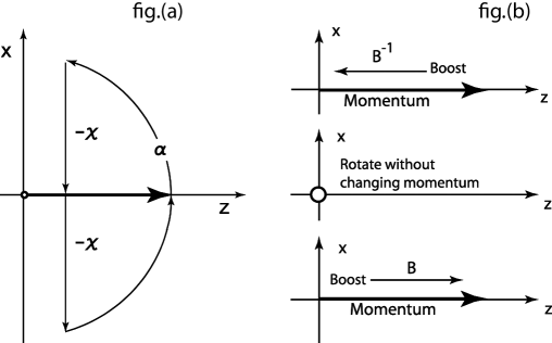
Figure 2: Bargmann and Wigner Decompositions. The Bargmann decomposition is illustrated in fig.(a). Starting from a momentum along the $z$ direction, we can rotate, boost, and rotate to bring the momentum to the original position. The resulting matrix is the product of one boost and two rotation matrices. In the Wigner decomposition, the particle is boosted back to the frame where the Wigner transformation can be applied. Make a Wigner transformation there and come back to the original state of the momentum as illustrated in fig.(b). This process also can also be written as the product of three simple matrices.

Except the sign of $\chi$, the two-by-two matrices of Eq.(104) and Eq.(105) are identical with those given in Sec. 3.2. The only difference is the sign of the parameter $\chi$. We are thus ready to interpret this expression in terms of physics.

• If the particle is massive, the off-diagonal elements of Eq.(105) have opposite signs, and this matrix can be decomposed into

  $$\pmatrix{e^{\eta/2}&0\cr 0&e^{-\eta/2}}\pmatrix{\cos(\theta/2)&-\sin(\theta/2)\cr\sin(\theta/2)&\cos(\theta/2)}\pmatrix{e^{\eta/2}&0\cr 0&e^{-\eta/2}}.$$ (106)

  with

  $$\cos(\theta/2)=(\cosh\chi)\cos\alpha,\quad\mbox{and}\quad e^{2\eta}=\frac{\cosh(\chi)\sin\alpha+\sinh\chi}{\cosh(\chi)\sin\alpha-\sinh\chi},$$ (107)

  and

  $$e^{2\eta}=\frac{p_{0}+p_{z}}{p_{0}-p_{z}}.$$ (108)

  According to Eq.(106) the first matrix (far right) reduces the particle momentum to zero. The second matrix rotates the particle without changing the momentum. The third matrix boosts the particle to restore its original momentum. This is the extension of Wigner’s original idea to moving particles.

• If the particle has an imaginary mass, the off-diagonal elements of Eq.(105) have the same sign,

  $$\pmatrix{e^{\eta/2}&0\cr 0&e^{-\eta/2}}\pmatrix{\cosh(\lambda/2)&-\sinh(\lambda/2)\cr\sinh(\lambda/2)&\cosh(\lambda/2)}\pmatrix{e^{\eta/2}&0\cr 0&e^{-\eta/2}},$$ (109)

  with

  $$\cosh(\lambda/2)=(\cosh\chi)\cos\alpha,\quad\mbox{and}\quad e^{2\eta}=\frac{\sinh\chi+\cosh(\chi)\sin\alpha}{\cosh(\chi)\sin\alpha-\sinh\chi},$$ (110)

  and

  $$e^{2\eta}=\frac{p_{0}+p_{z}}{p_{z}-p_{0}}.$$ (111)

  This is also a three-step operation. The first matrix brings the particle momentum to the zero-energy state with $p_{0}=0$. Boosts along the $x$ or $y$ direction do not change the four-momentum. We can then boost the particle back to restore its momentum. This operation is also an extension of the Wigner’s original little group. Thus, it is quite appropriate to call the formulas of Eq.(106) and Eq.(109) Wigner decompositions.

• If the particle mass is zero with

  $$\sinh\chi=(\cosh\chi)\sin\alpha,$$ (112)

  the $\eta$ parameter becomes infinite, and the Wigner decomposition does not appear to be useful. We can then go back to the Bargmann decomposition of Eq.(104). With the condition of Eq.(112), Eq.(105) becomes

  $$\pmatrix{1&-\gamma\cr 0&1},$$ (113)

  with

  $$\gamma=2\sinh\chi.$$ (114)

  The decomposition ending with a triangular matrix is called the Iwasawa decomposition [17, 22] and its physical interpretation was given in Subsec. 5.2. The $\gamma$ parameter does not depend on $\eta.$

Thus, we have given physical interpretations to the Bargmann and Wigner decompositions given in Sec. (3.2). Consider what happens when the momentum becomes large. Then $\eta$ becomes large for nonzero mass cases. All three four-momenta in Eq.(103) become

$$e^{\eta}\pmatrix{1&0\cr 0&0}.$$ (115)

As for the Bargmann-Wigner matrices, they become the triangular matrix of Eq.(113), with $\gamma=\sin(\theta/2)e^{\eta}$ and $\gamma=\sinh(\lambda/2)e^{\eta},$ respectively for the massive and imaginary-mass cases.

In Subsec. 5.2, we concluded that the triangular matrix corresponds to gauge transformations. However, particles with imaginary mass are not observed. For massive particles, we can start with the three-dimensional rotation group. The rotation around the $z$ axis is called helicity, and remains invariant under the boost along the $z$ direction. As for the transverse rotations, they become gauge transformation as illustrated in Table 6.

Table 6: Covariance of the energy-momentum relation, and covariance of the internal space-time symmetry. Under the Lorentz boost along the $z$ direction, $J_{3}$ remains invariant, and this invariant component of the angular momentum is called the helicity. The transverse component $J_{1}$ and $J_{2}$ collapse into a gauge transformation. The $\gamma$ parameter for the massless case has been studied in earlier papers in the four-by-four matrix formulation [8, 21].

Massive, Slow		COVARIANCE		Massless, Fast
$E=p^{2}/2m$		Einstein’s $E=mc^{2}$		$E=cp$
$J_{3}$				Helicity
		Wigner’s Little Group
$J_{1},J_{2}$				Gauge Transformation

5.4 Conjugate Transformations

The most general form of the $SL(2,c)$ matrix is given in Eq.(63). Transformation operators for the Lorentz group are given in exponential form as:

$$D=\exp{\left\{-i\sum_{i=1}^{3}\left(\theta_{i}J_{i}+\eta_{i}K_{i}\right)\right\}},$$ (116)

where the $J_{i}$ are the generators of rotations and the $K_{i}$ are the generators of proper Lorentz boosts. They satisfy the Lie algebra given in Eq.(42). This set of commutation relations is invariant under the sign change of the boost generators $K_{i}$. Thus, we can consider “dot conjugation” defined as

$$\dot{D}=\exp{\left\{-i\sum_{i=1}^{3}\left(\theta_{i}J_{i}-\eta_{i}K_{i}\right)\right\}},$$ (117)

Since $K_{i}$ are anti-Hermitian while $J_{i}$ are Hermitian, the Hermitian conjugate of the above expression is

$$D^{\dagger}=\exp{\left\{-i\sum_{i=1}^{3}\left(-\theta_{i}J_{i}+\eta_{i}K_{i}\right)\right\}},$$ (118)

while the Hermitian conjugate of $G$ is

$$\dot{D}^{\dagger}=\exp{\left\{-i\sum_{i=1}^{3}\left(-\theta_{i}J_{i}-\eta_{i}K_{i}\right)\right\}},$$ (119)

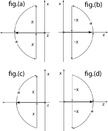
Figure 3: Four D-loops resulting from the Bargmann decomposition. Let us go back to Fig. 2. If we reverse of the direction of the boost, the result is fig.(a). From fig.(a), if we invert the space, we come back to fig.(b). If we reverse the direction of rotation from fig.(a), the result is fig.(c). If both the rotation and space are reversed, the result is the fig.(d).

Since we understand the rotation around the $z$ axis, we can now restrict the kinematics to the $zt$ plane, and work with the $Sp(2)$ symmetry. Then the $D$ matrices can be considered as Bargmann decompositions. First, $D$ and $\dot{D}$, and their Hermitian conjugates are

$$D(\alpha,\chi)=\pmatrix{(\cos\alpha)\cosh\chi&\sinh\chi-(\sin\alpha)\cosh\chi\cr\sinh\chi+(\sin\alpha)\cosh\chi&(\cos\alpha)\cosh\chi},$$ (120)

$$\dot{D}(\alpha,\chi)=\pmatrix{(\cos\alpha)\cosh\chi&-\sinh\chi-(\sin\alpha)\cosh\chi\cr-\sinh\chi+(\sin\alpha)\cosh\chi&(\cos\alpha)\cosh\chi}.$$

These matrices correspond to the “D loops” given in fig.(a) and fig.(b) of Fig. 3 respectively. The “dot” conjugation changes the direction of boosts. The dot conjugation leads to the inversion of the space which is called the parity operation.

We can also consider changing the direction of rotations. Then they result in the Hermitian conjugates. We can write their matrices as

$$D^{\dagger}(\alpha,\chi)=\pmatrix{(\cos\alpha)\cosh\chi&\sinh\chi+(\sin\alpha)\cosh\chi\cr\sinh\chi-(\sin\alpha)\cosh\chi&(\cos\alpha)\cosh\chi},$$

$$\dot{D}^{\dagger}(\alpha,\chi)=\pmatrix{(\cos\alpha)\cosh\chi&-\sinh\chi+(\sin\alpha)\cosh\chi\cr-\sinh\chi-(\sin\alpha)\cosh\chi&(\cos\alpha)\cosh\chi}.$$ (121)

From the exponential expressions from Eq.(116) to Eq.(119), it is clear that

$$D^{\dagger}=\dot{D}^{-1},\quad\mbox{and}\quad\dot{D}^{\dagger}=D^{-1}.$$ (122)

The D loop given in Fig. 2 corresponds to $\dot{D}$. We shall return to these loops in Sec. 7.

6 Symmetries derivable from the Poincaré Sphere

The Poincaré sphere serves as the basic language for polarization physics. Its underlying language is the two-by-two coherency matrix. This coherency matrix contains the symmetry of $SL(2,c)$ isomorphic to the the Lorentz group applicable to three space-like and one time-like dimensions [4, 6, 7].

For polarized light propagating along the $z$ direction, the amplitude ratio and phase difference of electric field $x$ and $y$ components traditionally determine the state of polarization. Hence, the polarization can be changed by adjusting the amplitude ratio or the phase difference or both. Usually, the optical device which changes amplitude is called an “attenuator” (or “amplifier”) and the device which changes the relative phase a “phase shifter.”

Let us start with the Jones vector:

$$\pmatrix{\psi_{1}(z,t)\cr\psi_{2}(z,t)}=\pmatrix{a\exp{[i(kz-\omega t)]}\cr a\exp{[i(kz-\omega t)]}}.$$ (123)

To this matrix, we can apply the phase shift matrix of Eq.(76) which brings the Jones vector to

$$\pmatrix{\psi_{1}(z,t)\cr\psi_{2}(z,t)}=\pmatrix{a\exp{[i(kz-\omega t-i\phi/2)]}\cr a\exp{[i(kz-\omega t+i\phi/2)]}}.$$ (124)

The generator of this phase-shifter is $J_{3}$ given Table 5.

The optical beam can be attenuated differently in the two directions. The resulting matrix is

$$e^{-\mu}\pmatrix{e^{\eta/2}&0\cr 0&e^{-\eta/2}}$$ (125)

with the attenuation factor of $\exp{\left(-\mu_{0}+\eta/2\right)}$ and $\exp{\left(-\mu-\eta/2\right)}$ for the $x$ and $y$ directions respectively. We are interested only the relative attenuation given in Eq.(45) which leads to different amplitudes for the $x$ and $y$ component, and the Jones vector becomes

$$\pmatrix{\psi_{1}(z,t)\cr\psi_{2}(z,t)}=\pmatrix{ae^{\mu/2}\exp{[i(kz-\omega t-i\phi/2)]}\cr ae^{-\mu/2}\exp{[i(kz-\omega t+i\phi/2)]}}.$$ (126)

The squeeze matrix of Eq.(45) is generated by $K_{3}$ given in Table 1.

The polarization is not always along the $x$ and $y$ axes, but can be rotated around the $z$ axis using Eq.(76) generated by $J_{2}$ given in Table 1.

Among the rotation angles, the angle of $45^{o}$ plays an important role in polarization optics. Indeed, if we rotate the squeeze matrix of Eq.(45) by $45^{o}$, we end up with the squeeze matrix of Eq.(44) generated by $K_{1}$ given also in Table 1.

Each of these four matrices plays an important role in special relativity, as we discussed in Secs. 3.2 and 7. Their respective roles in optics and particle physics are given in Table 7.

The most general form for the two-by-two matrix applicable to the Jones vector is the $G$ matrix of Eq.(63). This matrix is of course a representation of the $SL(2,c)$ group. It brings the simplest Jones vector of Eq.(123) to its most general form.

Table 7: Polarization optics and special relativity share the same mathematics. Each matrix has its clear role in both optics and relativity. The determinant of the Stokes or the four-momentum matrix remains invariant under Lorentz transformations. It is interesting to note that the decoherence parameter (least fundamental) in optics corresponds to the $(mass)^{2}$ (most fundamental) in particle physics.

Polarization Optics		Transformation Matrix		Particle Symmetry
Phase shift by $\phi$		$\pmatrix{e^{-i\phi/2}&0\cr 0&e^{i\phi/2}}$		Rotation around $z$.
Rotation around $z$		$\pmatrix{\cos(\theta/2)&-\sin(\theta/2)\cr\sin(\theta/2)&\cos(\theta/2)}$		Rotation around $y$.
Squeeze along $x$ and $y$		$\pmatrix{e^{\eta/2}&0\cr 0&e^{-\eta/2}}$		Boost along $z$.
Squeeze along $45^{o}$		$\pmatrix{\cosh(\lambda/2)&\sinh(\lambda/2)\cr\sinh(\lambda/2)&\cosh(\lambda/2)}$		Boost along $x$.
a4 $(\sin\xi)^{2}$		Determinant		(mass)2

6.1 Coherency Matrix

However, the Jones vector alone cannot tell us whether the two components are coherent with each other. In order to address this important degree of freedom, we use the coherency matrix defined as [3, 23]

$$C=\pmatrix{S_{11}&S_{12}\cr S_{21}&S_{22}},$$ (127)

where

$$<\psi_{i}^{*}\psi_{j}>=\frac{1}{T}\int_{0}^{T}\psi_{i}^{*}(t+\tau)\psi_{j}(t)dt,$$ (128)

where $T$ is a sufficiently long time interval. Then, those four elements become [4]

$$S_{11}=<\psi_{1}^{*}\psi_{1}>=a^{2},\qquad S_{12}=<\psi_{1}^{*}\psi_{2}>=a^{2}(\cos\xi)e^{-i\phi},$$

$$S_{21}=<\psi_{2}^{*}\psi_{1}>=a^{2}(\cos\xi)e^{+i\phi},\qquad S_{22}=<\psi_{2}^{*}\psi_{2}>=a^{2}.$$ (129)

The diagonal elements are the absolute values of $\psi_{1}$ and $\psi_{2}$ respectively. The angle $\phi$ could be different from the value of the phase-shift angle given in Eq.(76), but this difference does not play any role in the reasoning. The off-diagonal elements could be smaller than the product of $\psi_{1}$ and $\psi_{2}$, if the two polarizations are not completely coherent.

The angle $\xi$ specifies the degree of coherency. If it is zero, the system is fully coherent, while the system is totally incoherent if $\xi$ is $90^{o}$. This can therefore be called the “decoherence angle.”

While the most general form of the transformation applicable to the Jones vector is $G$ of Eq.(63), the transformation applicable to the coherency matrix is

$$C^{\prime}=G~{}C~{}G^{\dagger}.$$ (130)

The determinant of the coherency matrix is invariant under this transformation, and it is

$$\det(C)=a^{4}(\sin\xi)^{2}.$$ (131)

Thus, angle $\xi$ remains invariant. In the language of the Lorentz transformation applicable to the four-vector, the determinant is equivalent to the $(mass)^{2}$ and is therefore a Lorentz-invariant quantity.

6.2 Two Radii of the Poincaré Sphere

Let us write explicitly the transformation of Eq.(130) as

$$\pmatrix{S^{\prime}_{11}&S^{\prime}_{12}\cr S^{\prime}_{21}&S^{\prime}_{22}}=\pmatrix{\alpha&\beta\cr\gamma&\delta}\pmatrix{S_{11}&S_{12}\cr S_{21}&S_{22}}\pmatrix{\alpha^{*}&\gamma^{*}\cr\beta^{*}&\delta^{*}}.$$ (132)

It is then possible to construct the following quantities,

$$S_{0}=\frac{S_{11}+S_{22}}{2},\qquad S_{3}=\frac{S_{11}-S_{22}}{2},$$

$$S_{1}=\frac{S_{12}+S_{21}}{2},\qquad S_{2}=\frac{S_{12}-S_{21}}{2i}.$$ (133)

These are known as the Stokes parameters, and constitute a four-vector $\left(S_{0},S_{3},S_{1},S_{2}\right)$ under the Lorentz transformation.

Returning to Eq.(76), the amplitudes of the two orthogonal component are equal, thus, the two diagonal elements of the coherency matrix are equal. This leads to $S_{3}=0$, and the problem is reduced from the sphere to a circle.

In this two-dimensional subspace, we can introduce the polar coordinate system with

$$R=\sqrt{S_{1}^{2}+S_{2}^{2}}$$

$$S_{1}=R\cos\phi,$$

$$S_{2}=R\sin\phi.$$ (134)

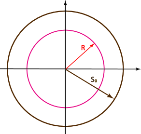
Figure 4: Radius of the Poincaré sphere. The radius $R$ takes its maximum value $S_{0}$ when the decoherence angle $\xi$ is zero. It becomes smaller as $\xi$ increases. It becomes zero when the angle reaches $90^{o}$.

The radius $R$ is the radius of this circle, and is

$$R=a^{2}\cos\xi.$$ (135)

The radius $R$ takes its maximum value $S_{0}$ when $\xi=0^{o}$. It decreases as $\xi$ increases and vanishes when $\xi=90^{o}$. This aspect of the radius R is illustrated in Fig. 4.

In order to see its implications in special relativity, let us go back to the four-momentum matrix of $m(1,0,0,0)$. Its determinant is $m^{2}$ and remains invariant. Likewise, the determinant of the coherency matrix of Eq.(127) should also remain invariant. The determinant in this case is

$$S_{0}^{2}-R^{2}=a^{4}\sin^{2}\xi.$$ (136)

This quantity remains invariant under the Hermitian transformation of Eq.(132), which is a Lorentz transformation as discussed in Secs. 3.2 and 7. This aspect is shown on the last row of Table 7.

The coherency matrix then becomes

$$C=a^{2}\pmatrix{1&(\cos\xi)e^{-i\phi}\cr(\cos\xi)e^{i\phi}&1}.$$ (137)

Since the angle $\phi$ does not play any essential role, we can let $\phi=0$, and write the coherency matrix as

$$C=a^{2}\pmatrix{1&\cos\xi\cr\cos\xi&1}.$$ (138)

The determinant of the above two-by-two matrix is

$$a^{4}\left(1-\cos^{2}\xi\right)=a^{4}\sin^{2}\xi.$$ (139)

Since the Lorentz transformation leaves the determinant invariant, the change in this $\xi$ variable is not a Lorentz transformation. It is of course possible to construct a larger group in which this variable plays a role in a group transformation [6], but here we are more interested in its role in a particle gaining a mass from zero or the mass becoming zero.

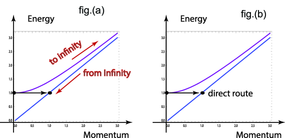
Figure 5: Transition from the massive to massless case. Within the framework of the Lorentz group, it is not possible to go from the massive to massless case directly, because it requires the change in the mass which is a Lorentz-invariant quantity. The only way is to move to infinite momentum and jump from the hyperbola to the light cone, and come back, as illustrated in fig.(a). The extra symmetry of the Poincaré sphere allows a direct transition as shown in fig. (b).

6.3 Extra-Lorentzian Symmetry

The coherency matrix of Eq.(137) can be diagonalized to

$$a^{2}\pmatrix{1+\cos\xi&0\cr 0&1-\cos\xi}$$ (140)

by a rotation. Let us then go back to the four-momentum matrix of Eq.(67). If $p_{x}=p_{y}=0$, and $p_{z}=p_{0}\cos\xi$ , we can write this matrix as

$$p_{0}\pmatrix{1+\cos\xi&0\cr 0&1-\cos\xi}.$$ (141)

Thus, with this extra variable, it is possible to study the little groups for variable masses, including the small-mass limit and the zero-mass case.

For a fixed value of $p_{0}$, the $(mass)^{2}$ becomes

$$(mass)^{2}=\left(p_{0}\sin\xi\right)^{2},\quad\mbox{and}\quad(momentum)^{2}=\left(p_{0}\cos\xi\right)^{2},$$ (142)

resulting in

$$(energy)^{2}=(mass)^{2}+(momentum)^{2}.$$ (143)

This transition is illustrated in Fig. 5. We are interested in reaching a point on the light cone from mass hyperbola while keeping the energy fixed. According to this figure, we do not have to make an excursion to infinite-momentum limit. If the energy is fixed during this process, Eq.(143) tells the mass and momentum relation, and Figure 6 illustrates this relation.

Within the framework of the Lorentz group, it is possible, by making an excursion to infinite momentum where the mass hyperbola coincides with the light cone, to then come back to the desired point. On the other hand, the mass formula of Eq.(142) allows us to go there directly. The decoherence mechanism of the coherency matrix makes this possible.

Figure 6: Energy-momentum-mass relation. This circle illustrates the case where the energy is fixed, while the mass and momentum are related according to the triangular rule. The value of the angle $\xi$ changes from zero to $180^{o}$. The particle mass is negative for negative values of this angle. However, in the Lorentz group, only $(mass)^{2}$ is a relevant variable, and negative masses might play a role for theoretical purposes.

7 Small-mass and Massless Particles

We now have a mathematical tool to reduce the mass of a massive particle from its positive value to zero. During this process, the Lorentz-boosted rotation matrix becomes a gauge transformation for the spin-1 particle, as discussed Subsec. 5.2. For spin-1/2 particles, there are two issues.

• It was seen in Subsec. 5.2 that the requirement of gauge invariance lead to a polarization of massless spin-1/2 particle, such as neutrinos. What happens to anti-neutrinos?

• There are strong experimental indications that neutrinos have a small mass. What happens to the $E(2)$ symmetry?

7.1 Spin-1/2 Particles

Let us go back to the two-by-two matrices of Subsec. 5.4, and the two-by-two $D$ matrix. For a massive particle, its Wigner decomposition leads to

$$D=\pmatrix{\cos(\theta/2)&-e^{-\eta}\sin(\theta/2)\cr e^{\eta}\sin(\theta/2)&\cos(\theta/2)}$$ (144)

This matrix is applicable to the spinors $u$ and $v$ defined in Eq.(98) respectively for the spin-up and spin-down states along the $z$ direction.

Since the Lie algebra of $SL(2,c)$ is invariant under the sign change of the $K_{i}$ matrices, we can consider the “dotted” representation, where the system is boosted in the opposite direction, while the direction of rotations remain the same. Thus, the Wigner decomposition leads to

$$\dot{D}=\pmatrix{\cos(\theta/2)&-e^{\eta}\sin(\theta/2)\cr e^{-\eta}\sin(\theta/2)&\cos(\theta/2)}$$ (145)

with its spinors

$$\dot{u}=\pmatrix{1\cr 0},\quad\mbox{and}\quad\dot{v}=\pmatrix{0\cr 1}.$$ (146)

For anti-neutrinos, the helicity is reversed but the momentum is unchanged. Thus, $D^{\dagger}$ is the appropriate matrix. However, $D^{\dagger}=\dot{D}^{-1}$ as was noted in Subsec 5.4. Thus, we shall use $\dot{D}$ for anti-neutrinos.

When the particle mass becomes very small,

$$e^{-\eta}=\frac{m}{2p},$$ (147)

becomes small. Thus, if we let

$$e^{\eta}\sin(\theta/2)=\gamma,\quad\mbox{and}\quad e^{-\eta}\sin(\theta/2)=\epsilon^{2},$$ (148)

then the $D$ matrix of Eq.(144) and the $\dot{D}$ of Eq.(145) become

$$\pmatrix{1-\gamma\epsilon^{2}/2&-\epsilon^{2}\cr\gamma&1-\gamma\epsilon^{2}},\quad\mbox{and}\quad\pmatrix{1-\gamma\epsilon^{2}/2&-\gamma\cr\epsilon^{2}&1-\gamma\epsilon^{2}},$$ (149)

respectively where $\gamma$ is an independent parameter and

$$\epsilon^{2}=\gamma\left(\frac{m}{2p}\right)^{2}.$$ (150)

When the particle mass becomes zero, they become

$$\pmatrix{1&0\cr\gamma&1},\quad\mbox{and}\quad\pmatrix{1&-\gamma\cr 0&1},$$ (151)

respectively, applicable to the spinors $(u,v)$ and $(\dot{u},\dot{v})$ respectively.

For neutrinos,

$$\pmatrix{1&0\cr\gamma&1}\pmatrix{1\cr 0}=\pmatrix{1\cr\gamma},\quad\mbox{and}\quad\pmatrix{1&0\cr\gamma&1}\pmatrix{0\cr 1}=\pmatrix{0\cr 1}.$$ (152)

For anti-neutrinos,

$$\pmatrix{1&-\gamma\cr 0&1}\pmatrix{1\cr 0}=\pmatrix{1\cr 0},\quad\mbox{and}\quad\pmatrix{1&-\gamma\cr 0&1}\pmatrix{0\cr 1}=\pmatrix{-\gamma\cr 1}.$$ (153)

It was noted in Subsec. 5.2 that the triangular matrices of Eq.(151) perform gauge transformations. Thus, for Eq.(152) and Eq.(153) the requirement of gauge invariance leads to the polarization of neutrinos. The neutrinos are left-handed while the anti-neutrinos are right-handed. Since, however, nature cannot tell the difference between the dotted and undotted representations, the Lorentz group cannot tell which neutrino is right handed. It can say only that the neutrinos and anti-neutrinos are oppositely polarized.

If the neutrino has a small mass, the gauge invariance is modified to

$$\pmatrix{1-\gamma\epsilon^{2}/2&-\epsilon^{2}\cr\gamma&1-\gamma\epsilon^{2}/2}\pmatrix{0\cr 1}=\pmatrix{0\cr 1}-\epsilon^{2}\pmatrix{1\cr\gamma/2},$$ (154)

and

$$\pmatrix{1-\gamma\epsilon^{2}/2&-\gamma\cr\epsilon^{2}&1-\gamma\epsilon^{2}}\pmatrix{1\cr 0}=\pmatrix{1\cr 0}+\epsilon^{2}\pmatrix{-\gamma/2\cr 1},$$ (155)

respectively for neutrinos and anti-neutrinos. Thus the violation of the gauge invariance in both cases is proportional to $\epsilon^{2}$ which is $m^{2}/4p^{2}$.

7.2 Small-mass neutrinos in the Real World

Whether neutrinos have mass or not and the consequences of this relative to the Standard Model and lepton number is the subject of much theoretical speculation [24, 25], and of cosmology [26], nuclear reactors [27, 28], and high energy experimentations [29, 30]. Neutrinos are fast becoming an important component of the search for dark matter and dark radiation [31]. Their importance within the Standard Model is reflected by the fact that they are the only particles which seem to exist with only one direction of chirality, i.e. only left-handed neutrinos have been confirmed to exist so far.

It was speculated some time ago that neutrinos in constant electric and magnetic fields would acquire a small mass, and that right-handed neutrinos would be trapped within the interaction field [32]. Solving generalized electroweak models using left- and right-handed neutrinos has been discussed recently [33]. Today these right-handed neutrinos which do not participate in weak interactions are called “sterile” neutrinos [34]. A comprehensive discussion of the place of neutrinos in the scheme of physics has been given by Drewes [31].

8 Scalars, Four-vectors, and Four-Tensors

In Secs. 5 and 7, our primary interest has been the two-by-two matrices applicable to spinors for spin-1/2 particles. Since we also used four-by-four matrices, we indirectly studied the four-component particle consisting of spin-1 and spin-zero components.

If there are two spin 1/2 states, we are accustomed to construct one spin-zero state, and one spin-one state with three degeneracies.

In this paper, we are confronted with two spinors, but each spinor can also be dotted. For this reason, there are sixteen orthogonal states consisting of spin-one and spin-zero states. How many spin-zero states? How many spin-one states?

For particles at rest, it is known that the addition of two one-half spins result in spin-zero and spin-one states. In the this paper, we have two different spinors behaving differently under the Lorentz boost. Around the $z$ direction, both spinors are transformed by

$$Z(\phi)=\exp{\left(-i\phi J_{3}\right)}=\pmatrix{e^{-i\phi/2}&0\cr 0&e^{i\phi/2}}.$$ (156)

However, they are boosted by

$$B(\eta)=\exp{\left(-i\eta K_{3}\right)}=\pmatrix{e^{\eta/2}&0\cr 0&e^{-\eta/2}},$$

$$\dot{B}(\eta)=\exp{\left(i\eta K_{3}\right)},=\pmatrix{e^{-\eta/2}&0\cr 0&e^{\eta/2}}$$ (157)

applicable to the undotted and dotted spinors respectively. These two matrices commute with each other, and also with the rotation matrix $Z(\phi)$ of Eq.(156). Since $K_{3}$ and $J_{3}$ commute with each other, we can work with the matrix $Q(\eta,\phi)$ defined as

$$Q(\eta,\phi)=B(\eta)Z(\phi)=\pmatrix{e^{(\eta-i\phi)/2}&0\cr 0&e^{-(\eta-i\phi)/2}},$$

$$\dot{Q}(\eta,\phi)=\dot{B}(\eta)\dot{Z}(\phi)=\pmatrix{e^{-(\eta+i\phi)/2}&0\cr 0&e^{(\eta+i\phi)/2}}.$$ (158)

When this combined matrix is applied to the spinors,

$$Q(\eta,\phi)u=e^{(\eta-i\phi)/2}u,\qquad Q(\eta,\phi)v=e^{-(\eta-i\phi)/2}v,$$

$$\dot{Q}(\eta,\phi)\dot{u}=e^{-(\eta+i\phi)/2}\dot{u},\qquad\dot{Q}(\eta,\phi)\dot{v}=e^{(\eta+i\phi)/2}\dot{v}.$$ (159)

If the particle is at rest, we can construct the combinations

$$uu,\qquad\frac{1}{\sqrt{2}}(uv+vu),\qquad vv,$$ (160)

to construct the spin-1 state, and

$$\frac{1}{\sqrt{2}}(uv-vu),$$ (161)

for the spin-zero state. There are four bilinear states. In the $SL(2,c)$ regime, there are two dotted spinors. If we include both dotted and undotted spinors, there are sixteen independent bilinear combinations. They are given in Table 8. This table also gives the effect of the operation of $Q(\eta,\phi)$.

Table 8: Sixteen combinations of the $SL(2,c)$ spinors. In the $SU(2)$ regime, there are two spinors leading to four bilinear forms. In the $SL(2,c)$ world, there are two undotted and two dotted spinors. These four spinors lead to sixteen independent bilinear combinations.

	Spin 1		Spin 0
	$uu,\quad\frac{1}{\sqrt{2}}(uv+vu),\quad vv,$		$\frac{1}{\sqrt{2}}(uv-vu)$
	$\dot{u}\dot{u},\quad\frac{1}{\sqrt{2}}(\dot{u}\dot{v}+\dot{v}\dot{u}),\quad\dot{v}\dot{v},$		$\frac{1}{\sqrt{2}}(\dot{u}\dot{v}-\dot{v}\dot{u})$
	$u\dot{u},\quad\frac{1}{\sqrt{2}}(u\dot{v}+v\dot{u}),\quad v\dot{v},$		$\frac{1}{\sqrt{2}}(u\dot{v}-v\dot{u})$
	$\dot{u}u,\quad\frac{1}{\sqrt{2}}(\dot{u}v+\dot{v}u),\quad\dot{v}v,$		$\frac{1}{\sqrt{2}}(\dot{u}v-\dot{v}u)$
	After the operation of $Q(\eta,\phi)$ and $\dot{Q}(\eta,\phi)$
	$e^{-i\phi}e^{\eta}uu,\quad\frac{1}{\sqrt{2}}(uv+vu),\quad e^{i\phi}e^{-\eta}vv,$		$\frac{1}{\sqrt{2}}(uv-vu)$
	$e^{-i\phi}e^{-\eta}\dot{u}\dot{u},\quad\frac{1}{\sqrt{2}}(\dot{u}\dot{v}+\dot{v}\dot{u}),\quad e^{i\phi}e^{\eta}\dot{v}\dot{v},$		$\frac{1}{\sqrt{2}}(\dot{u}\dot{v}-\dot{v}\dot{u})$
	$e^{-i\phi}u\dot{u},\quad\frac{1}{\sqrt{2}}(e^{\eta}u\dot{v}+e^{-\eta}v\dot{u}),\quad e^{i\phi}v\dot{v},$		$\frac{1}{\sqrt{2}}(e^{\eta}u\dot{v}-e^{-\eta}v\dot{u})$
	$e^{-i\phi}\dot{u}u,\quad\frac{1}{\sqrt{2}}(\dot{u}v+\dot{v}u),\quad e^{i\phi}\dot{v}v,$		$\frac{1}{\sqrt{2}}(e^{-\eta}\dot{u}v-e^{\eta}\dot{v}u)$

Among the bilinear combinations given in Table 8, the following two are invariant under rotations and also under boosts.

$$S=\frac{1}{\sqrt{2}}(uv-vu),\quad\mbox{and}\quad\dot{S}=-\frac{1}{\sqrt{2}}(\dot{u}\dot{v}-\dot{v}\dot{u}).$$ (162)

They are thus scalars in the Lorentz-covariant world. Are they the same or different? Let us consider the following combinations

$$S_{+}=\frac{1}{\sqrt{2}}\left(S+\dot{S}\right),\quad\mbox{and}\quad S_{-}=\frac{1}{\sqrt{2}}\left(S-\dot{S}\right).$$ (163)

Under the dot conjugation, $S_{+}$ remains invariant, but $S_{-}$ changes its sign.

Under the dot conjugation, the boost is performed in the opposite direction. Therefore it is the operation of space inversion, and $S_{+}$ is a scalar while $S_{-}$ is called the pseudo-scalar.

8.1 Four-vectors

Let us consider the bilinear products of one dotted and one undotted spinor as  $u\dot{u},~{}u\dot{v},~{}\dot{u}v,~{}v\dot{v}$, and construct the matrix

$$U=\pmatrix{u\dot{v}&v\dot{v}\cr u\dot{u}&v\dot{u}}.$$ (164)

Under the rotation $Z(\phi)$ and the boost $B(\eta)$ they become

$$\pmatrix{e^{\eta}u\dot{v}&e^{-i\phi}v\dot{v}\cr e^{i\phi}u\dot{u}&e^{-\eta}v\dot{u}}.$$ (165)

Indeed, this matrix is consistent with the transformation properties given in Table 8, and transforms like the four-vector

$$\pmatrix{t+z&x-iy\cr x+iy&t-z}.$$ (166)

This form was given in Eq.(62), and played the central role throughout this paper. Under the space inversion, this matrix becomes

$$\pmatrix{t-z&-(x-iy)\cr-(x+iy)&t+z}.$$ (167)

This space inversion is known as the parity operation.

The form of Eq.(164) for a particle or field with four-components, is given by $(V_{0},V_{z},V_{x},V_{y})$. The two-by-two form of this four-vector is

$$U=\pmatrix{V_{0}+V_{z}&V_{x}-iV_{y}\cr V_{x}+iV_{y}&V_{0}-V_{z}}.$$ (168)

If boosted along the $z$ direction, this matrix becomes

$$\pmatrix{e^{\eta}\left(V_{0}+V_{z}\right)&V_{x}-iV_{y}\cr V_{x}+iV_{y}&e^{-\eta}\left(V_{0}-V_{z}\right)}.$$ (169)

In the mass-zero limit, the four-vector matrix of Eq.(169) becomes

$$\pmatrix{2A_{0}&A_{x}-iA_{y}\cr A_{x}+iA_{y}&0},$$ (170)

with the Lorentz condition $A_{0}=A_{z}$. The gauge transformation applicable to the photon four-vector was discussed in detail in Subsec. 5.2.

Let us go back to the matrix of Eq.(168), we can construct another matrix $\dot{U}$. Since the dot conjugation leads to the space inversion,

$$\dot{U}=\pmatrix{\dot{u}v&\dot{v}v\cr\dot{u}u&\dot{v}u}.$$ (171)

Then

$$\dot{u}v\simeq(t-z),\qquad\dot{v}u\simeq(t+z)$$

$$\dot{v}v\simeq-(x-iy),\qquad\dot{u}u\simeq-(x+iy),$$ (172)

where the symbol $\simeq$ means “transforms like.”

Thus, $U$ of Eq.(164) and $\dot{U}$ of Eq.(171) used up eight of the sixteen bilinear forms. Since there are two bilinear forms in the scalar and pseudo-scalar as given in Eq.(163), we have to give interpretations to the six remaining bilinear forms.

8.2 Second-rank Tensor

In this subsection, we are studying bilinear forms with both spinors dotted and undotted. In Subsec. 8.1, each bilinear spinor consisted of one dotted and one undotted spinor. There are also bilinear spinors which are both dotted or both undotted. We are interested in two sets of three quantities satisfying the $O(3)$ symmetry. They should therefore transform like

$$(x+iy)/\sqrt{2},\qquad(x-iy)/\sqrt{2},\qquad z,$$ (173)

which are like

$$uu,\qquad vv,\quad(uv+vu)/\sqrt{2},$$ (174)

respectively in the $O(3)$ regime. Since the dot conjugation is the parity operation, they are like

$$-\dot{u}\dot{u},\qquad-\dot{v}\dot{v},\qquad-(\dot{u}\dot{v}+\dot{v}\dot{u})/\sqrt{2}.$$ (175)

In other words,

$$(uu{\dot{)}}=-\dot{u}\dot{u},\quad\mbox{and}\quad(vv{\dot{)}}=-\dot{v}\dot{v}.$$ (176)

We noticed a similar sign change in Eq.(8.1).

In order to construct the $z$ component in this $O(3)$ space, let us first consider

$$f_{z}=\frac{1}{2}\left[(uv+vu)-\left(\dot{u}\dot{v}+\dot{v}\dot{u}\right)\right],\qquad g_{z}=\frac{1}{2i}\left[(uv+vu)+\left(\dot{u}\dot{v}+\dot{v}\dot{u}\right)\right],$$ (177)

where $f_{z}$ and $g_{z}$ are respectively symmetric and anti-symmetric under the dot conjugation or the parity operation. These quantities are invariant under the boost along the $z$ direction. They are also invariant under rotations around this axis, but they are not invariant under boost along or rotations around the $x$ or $y$ axis. They are different from the scalars given in Eq.(162).

Next, in order to construct the $x$ and $y$ components, we start with $g_{\pm}$ as

$$f_{+}=\frac{1}{\sqrt{2}}\left(uu-\dot{u}\dot{u}\right)\qquad g_{+}=\frac{1}{\sqrt{2}i}\left(uu+\dot{u}\dot{u}\right)$$

$$f_{-}=\frac{1}{\sqrt{2}}\left(vv-\dot{v}\dot{v}\right)\qquad g_{-}=\frac{1}{\sqrt{2}i}\left(vv+\dot{v}\dot{v}\right).$$ (178)

Then

$$f_{x}=\frac{1}{\sqrt{2}}\left(f_{+}+f_{-}\right)=\frac{1}{2}\left[\left(uu-\dot{u}\dot{u}\right)+\left(vv-\dot{v}\dot{v}\right)\right]$$

$$f_{y}=\frac{1}{\sqrt{2}i}\left(f_{+}-f_{-}\right)=\frac{1}{2i}\left[\left(uu-\dot{u}\dot{u}\right)-\left(vv-\dot{v}\dot{v}\right)\right].$$ (179)

and

$$g_{x}=\frac{1}{\sqrt{2}}\left(g_{+}+g_{-}\right)=\frac{1}{2i}\left[\left(uu+\dot{u}\dot{u}\right)+\left(vv+\dot{v}\dot{v}\right)\right]$$

$$g_{y}=\frac{1}{\sqrt{2}i}\left(g_{+}-g_{-}\right)=-\frac{1}{2}\left[\left(uu+\dot{u}\dot{u}\right)-\left(vv+\dot{v}\dot{v}\right)\right].$$ (180)

Here $f_{x}$ and $f_{y}$ are symmetric under dot conjugation, while $g_{x}$ and $g_{y}$ are anti-symmetric.

Furthermore, $f_{z},f_{x},$ and $f_{y}$ of Eqs.(177) and (8.2) transform like a three-dimensional vector. The same can be said for $g_{i}$ of Eqs.(177) and (8.2). Thus, they can grouped into the second-rank tensor

$$T=\pmatrix{0&-g_{z}&-g_{x}&-g_{y}\cr g_{z}&0&-f_{y}&f_{x}\cr g_{x}&f_{y}&0&-f_{z}\cr g_{y}&-f_{x}&f_{z}&0},$$ (181)

whose Lorentz-transformation properties are well known. The $g_{i}$ components change their signs under space inversion, while the $f_{i}$ components remain invariant. They are like the electric and magnetic fields respectively.

If the system is Lorentz-booted, $f_{i}$ and $g_{i}$ can be computed from Table 8. We are now interested in the symmetry of photons by taking the massless limit. According to the procedure developed in Sec. 6, we can keep only the terms which become larger for larger values of $\eta$. Thus,

$$f_{x}\rightarrow\frac{1}{2}\left(uu-\dot{v}\dot{v}\right),\qquad f_{y}\rightarrow\frac{1}{2i}\left(uu+\dot{v}\dot{v}\right),$$

$$g_{x}\rightarrow\frac{1}{2i}\left(uu+\dot{v}\dot{v}\right),\qquad g_{y}\rightarrow-\frac{1}{2}\left(uu-\dot{v}\dot{v}\right),$$ (182)

in the massless limit.

Then the tensor of Eq.(181) becomes

$$F=\pmatrix{0&0&-E_{x}&-E_{y}\cr 0&0&-B_{y}&B_{x}\cr E_{x}&B_{y}&0&0\cr E_{y}&-B_{x}&0&0},$$ (183)

with

$$B_{x}\simeq\frac{1}{2}\left(uu-\dot{v}\dot{v}\right),\qquad B_{y}\simeq\frac{1}{2i}\left(uu+\dot{v}\dot{v}\right),$$

$$E_{x}=\frac{1}{2i}\left(uu+\dot{v}\dot{v}\right),\qquad E_{y}=-\frac{1}{2}\left(uu-\dot{v}\dot{v}\right).$$ (184)

The electric and magnetic field components are perpendicular to each other. Furthermore,

$$E_{x}=B_{y},\quad\mbox{\quad}E_{y}=-B_{x}.$$ (185)

In order to address this question, let us go back to Eq.(8.2). In the massless limit,

$$B_{+}\simeq E_{+}\simeq uu,\qquad B_{-}\simeq E_{-}\simeq\dot{v}\dot{v}$$ (186)

The gauge transformation applicable to $u$ and $\dot{v}$ are the two-by-two matrices

$$\pmatrix{1&-\gamma\cr 0&1},\quad\mbox{and}\quad\pmatrix{1&0\cr-\gamma&1}.$$ (187)

respectively as noted in Subsecs. 5.2 and 7.1. Both $u$ and $\dot{v}$ are invariant under gauge transformations, while $\dot{u}$ and $v$ do not.

The $B_{+}$ and $E_{+}$ are for the photon spin along the $z$ direction, while $B_{-}$ and $E_{-}$ are for the opposite direction. In 1964 [35], Weinberg constructed gauge-invariant state vectors for massless particles starting from Wigner’s 1939 paper [1]. The bilinear spinors $uu$ and and $\dot{v}\dot{v}$ correspond to Weinberg’s state vectors.

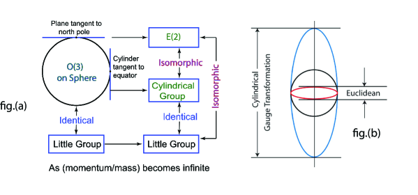
Figure 7: Contractions of the three-dimensional rotation group. This group can be illustrated by a sphere. This group can become the two-dimensional Euclidean group on a plane tangent at the north pole as illustrated in fig.(a). It was later noted that there is a cylinder tangential to this sphere, and the up and down translations on this cylinder correspond to the gauge transformation for photons [20]. As illustrated in fig.(b), the four-dimensional representation of of the Lorentz group contains both elongation and contraction of of the $z$ axis, as the system is boosted along this direction. The elongation and the contraction become the cylindrical and Euclidean groups, respectively [21].

8.3 Possible Symmetry of the Higgs Mechanism

In this section, we discussed how the two-by-two formalism of the group $SL(2,c)$ leads the scalar, four-vector, and tensor representations of the Lorentz group. We discussed in detail how the four-vector for a massive particle can be decomposed into the symmetry of a two-component massless particle and one gauge degree of freedom. This aspect was studied in detail by Kim and Wigner [20, 21], and their results are illustrated in Fig. 7.

This subject was initiated by Inönü and Wigner in 1953 as the group contraction [36]. In their paper, they discussed the contraction of the three-dimensional rotation group becoming contracted to the two-dimensional Euclidean group with one rotational and two translational degrees of freedom. While the $O(3)$ rotation group can be illustrated by a three-dimensional sphere, the plane tangential at the north pole is for the $E(2)$ Euclidean group. However, we can also consider a cylinder tangential at the equatorial belt. The resulting cylindrical group is isomorphic to the Euclidean group [20]. While the rotational degree of freedom of this cylinder is for the photon spin, the up and down translations on the surface of the cylinder correspond to the gauge degree of freedom of the photon, as illustrated in Fig. 7.

The four-dimensional Lorentz group contains both the Euclidean and cylindrical contractions. These contraction processes transform a four-component massive vector meson into a massless spin-one particle with two spin one-half components, and one gauge degree of freedom.

Since this contraction procedure is spelled out detail in Ref. [21], as well as in the present paper, its reverse process is also well understood. We start with one two-component massless particle with one gauge degree of freedom, and end up with a massive vector meson with its four components.

The mathematics of this process is not unlike the Higgs mechanism [37, 38], where one massless field with two degrees of freedom absorbs one gauge degree freedom to become a quartet of bosons, namely that of $W,Z^{\pm}$ plus the Higgs boson. As is well known, this mechanism is the basis for the theory of electro-weak interaction formulated by Weinberg and Salam [39, 40].

The word ”spontaneous symmetry breaking” is used for the Higgs mechanism. It could be an interesting problem to see that this symmetry breaking for the two Higgs doublet model can be formulated in terms of the Lorentz group and its contractions. In this connection, we note an interesting recent paper by Dée and Ivanov [41].

Conclusions

It was noted in this paper that the second-order differential equation for damped harmonic oscillators can be formulated in terms of two-by-two matrices. These matrices produce the algebra of the group $Sp(2)$. While there are three trace classes of the two-by-two matrices of this group, the damped oscillator tells us how to make transitions from one class to another.

It is shown that Wigner’s three little groups can be defined in terms of the trace classes of the $Sp(2)$ group. If the trace is smaller than two, the little group is for massive particles. If greater than two, the little group is for imaginary-mass particles. If the trace is equal to two, the little group is for massless particles. Thus, the damped harmonic oscillator provides a procedure for transition from one little group to another.

The Poincaré sphere contains the symmetry of the six-parameter $SL(2,c)$group. Thus, the sphere provides the procedure for extending the symmetry of the little group defined within the space of three-dimensional Lorentz group to the full four-dimensional Minkowski space. In addition, the Poincaré sphere offers the variable which allows us to change the symmetry of massive particle to that of massless particle by continuously changing the mass.

In this paper, we extracted the mathematical properties of the Lorentz group and Wigner’s little groups from the damped harmonic oscillator and the Poincaré sphere. In addition, it should be noted that the symmetry of the Lorentz group is also contained in the squeezed state of light [15] and the $ABCD$ matrix for optical beam transfers [14].

In addition, we mentioned the possibility of understanding the the mathematics of the Higgs mechanism in terms of the Lorentz group and its contractions.

References

- [1] Wigner, E. On Unitary Representations of the Inhomogeneous Lorentz Group, Ann. Math. 1939, 40, 149-204.
- [2] Han, D; Kim, Y. S.; Son, D. Eulerian parametrization of Wigner little groups and gauge transformations in terms of rotations in 2-component spinors, J. Math. Phys. 1986, 27, 2228-2235.
- [3] Born, M.; Wolf, E. Principles of Optics. 6th Ed. (Pergamon, Oxford) 1980.
- [4] Han, D; Kim, Y. S.; Noz, M. E. Stokes parameters as a Minkowskian four-vector, Phys. Rev. E 1997, 56, 6065-76.
- [5] Brosseau, C. Fundamentals of Polarized Light: A Statistical Optics Approach (John Wiley, New York) 1998.
- [6] Başkal, S; Kim, Y. S. de Sitter group as a symmetry for optical decoherence, J. Phys. A 2006, 39, 7775-88.
- [7] Kim, Y. S.; Noz, M. E. Symmetries Shared by the Poincaré Group and the Poincaré Sphere, Symmetry 2013, 5, 233-252.
- [8] Han, D; Kim, Y. S; Son, D. E(2)-like little group for massless particles and polarization of neutrinos, Phys. Rev. D 1982, 26, 3717-3725.
- [9] Han, D.; Kim Y. S.; Son D. Photons, neutrinos and gauge transformations, Am. J. Phys. 1986, 54, 818-821.
- [10] Başkal, S; Kim, Y. S. Little groups and Maxwell-type tensors for massive and massless particles, Europhys. Lett. 1997, 40, 375-380.
- [11] Leggett, A; Chakravarty, S; Dorsey, A; Fisher, M; Garg, A; Zwerger, W. Dynamics of the dissipative 2-state system, Rev. Mod. Phys. 1987, 59, 1-85.
- [12] Başkal, S.; Kim, Y. S. One analytic form for four branches of the ABCD matrix, J. Mod. Opt. 2010, 57, 1251-1259
- [13] Başkal, S.; Kim, Y. S. Lens optics and the continuity problems of the ABCD matrix J. Mod. Opt. 2014, 61, 161-166.
- [14] Başkal, S.; Kim, Y. S. Lorentz Group in Ray and Polarization Optics. Chapter 9 in Mathematical Optics: Classical, Quantum and Computational Methods edited by Vasudevan Lakshminarayanan, Maria L. Calvo, and Tatiana Alieva (CRC Taylor and Francis, New York) 2013, pp 303-340.
- [15] Kim, Y. S.; Noz, M. E. Theory and Applications of the Poincaré Group (Reidel, Dordrecht) 1986.
- [16] Bargmann, V. Irreducible unitary representations of the Lorentz group, Ann. Math. 1947, 48, 568-640.
- [17] Iwasawa, K. On Some Types of Topological Groups, Ann. Math. 1949 50, 507-558.
- [18] Guillemin, V.; Sternberg, S. Symplectic Techniques in Physics (Cambridge University Press, Cambridge) 1984).
- [19] Naimark, M. A. Linear Representations of the Lorentz Group, translated by Ann Swinfen and O. J. Marstrand (Pergamon Press)1964. The original book written in Russian was published by Fizmatgiz (Moscow) 1958.
- [20] Kim, Y. S.; Wigner, E. P. Cylindrical group and masless particles, J. Math. Phys. 1987, 28, 1175-1179.
- [21] Kim, Y. S.; Wigner, E.P. Space-time geometry of relativistic particles, J. Math. Phys. 1990, 31, 55-60.
- [22] Georgieva, E.; Kim, Y. S. Iwasawa effects in multilayer optics, Phys. Rev. E 2001, 64, 026602-026606.
- [23] Saleh, B. E. A.; Teich, M. C. Fundamentals of Photonics. 2nd Ed. (John Wiley, Hoboken, New Jersey) 2007.
- [24] Papoulias, D. K.; Kosmas, T. S. Exotic Lepton Flavour Violating Processes in the Presence of Nuclei, J. Phys.: Conference Series 2013, 410, 012123 1-5.
- [25] Dinh, D. N.; Petcov, S. T.; Sasao, N.; Tanaka, M.; Yoshimura, M. Observables in neutrino mass spectroscopy using atoms Phys. Lett. B. 2013, 719, 154-163.
- [26] Miramonti, L.; Antonelli, V. Advancements in Solar Neutrino physics Int. J. Mod. Phys. E. 2013, 22, 1-16.
- [27] Sinev, V. V. Joint analysis of spectral reactor neutrino experiments, arXiv:1103.2452v3 2013 1-8.
- [28] Li, Y-F.; Cao, J.; Jun, Y.; Wang, Y.; Zhan, L. Unambiguous Determination of the Neutrino Mass Hierarchy Using Reactor Neutrinos, Phys. Rev. D. 2013 88, 013008 1-9.
- [29] Bergstrom, J. Combining and comparing neutrinoless double beta decay experiments using different nuclei, arXiv:1212.4484v3 2013 1-23.
- [30] Han, T.; I. Lewis, I.; Ruiz, R.; and Si, Z-g. Lepton number violation and chiral couplings at the LHC, Phys. Rev. D 2013, 87, 03501,1 1-25.
- [31] Drewes, M. The Phenomenology of Right Handed Neutrinos, Int. J. Mod. Phys. E 2013, 22, 1330019 1-75.
- [32] Barut, A. O.; McEwan, J. The Four States of the Massless Neutrino with Pauli Coupling by Spin-gauge Invariance, Lett. Math. Phys. 1986, 11, 67-72.
- [33] Palcu, A. Neutrino Mass as a consequence of the exact solution of 3-3-1 gauge models without exotic electric charges, Mod. Phys. Lett. A. 2006, 21, 1203-1217.
- [34] Bilenky, S. M. Neutrino, Physics of Particles and Nuclei 2013, 44, 1-46.
- [35] Weinberg, S. Photons and Gravitons in S-Matrix Theory: Derivation of Charge Conservation and Equality of Gravitational and Inertial Mass, Phys. Rev. 1964, 135, B1049-B1056.
- [36] Inönü, E.; Wigner, E. P. On the Contraction of Groups and their Representations Proc. Natl. Acad. Sci. (U.S.) 1953, 39, 510-524.
- [37] Higgs, P. W. Broken symmetries and the masses of gauge bosons, Phys. Rev. Lett. 1964, 13, 508-509.
- [38] Guralnik, G. S.; Hagen, C. R.; Kibble, T. W. B. Global Conservation Laws and Massless Particles, Phys. Rev. Lett. 1964, 13, 585-587.
- [39] Weinberg, S. A model of leptons, Phys. Rev. Lett. 1967, 19, 1265-1266.
- [40] Weinberg, S. Quantum Theory of Fields, Volume II, Modern Applications (Cambridge University Press) 1996.
- [41] Dée, A; Ivanov, I. P. Higgs boson masses of the general two-Higgs-doublet model in the Minkowski-space formalism Phys. Rev. D 2010, 81, 015012-8.