Conservative L-systems and the Livšic function

Abstract.

We study the connection between the classes of (i) Livšic functions $s(z),$ i.e., the characteristic functions of densely defined symmetric operators $\dot{A}$ with deficiency indices $(1,1)$; (ii) the characteristic functions $S(z)$ of a maximal dissipative extension $T$ of $\dot{A},$ i.e., the Möbius transform of $s(z)$ determined by the von Neumann parameter $\kappa$ of the extension relative to an appropriate basis in the deficiency subspaces; and (iii) the transfer functions $W_{\Theta}(z)$ of a conservative L-system $\Theta$ with the main operator $T$. It is shown that under a natural hypothesis the functions $S(z)$ and $W_{\Theta}(z)$ are reciprocal to each other. In particular, $W_{\Theta}(z)=\frac{1}{S(z)}=-\frac{1}{s(z)}$ whenever $\kappa=0$. It is established that the impedance function of a conservative L-system with the main operator $T$ belongs to the Donoghue class if and only if the von Neumann parameter vanishes ($\kappa=0$). Moreover, we introduce the generalized Donoghue class and obtain the criteria for an impedance function to belong to this class. We also obtain the representation of a function from this class via the Weyl-Titchmarsh function. All results are illustrated by a number of examples.

1. Introduction

Suppose that $T$ is a densely defined closed operator in a Hilbert space ${\mathcal{H}}$ such that its resolvent set $\rho(T)$ is not empty and assume, in addition, that $\text{\rm{Dom}}(T)\cap\text{\rm{Dom}}(T^{*})$ is dense. We also suppose that the restriction ${\dot{A}}=T|_{\text{\rm{Dom}}(T)\cap\text{\rm{Dom}}(T^{*})}$ is a closed symmetric operator with finite equal deficiency indices and that ${\mathcal{H}}_{+}\subset{\mathcal{H}}\subset{\mathcal{H}}_{-}$ is the rigged Hilbert space associated with $\dot{A}$ (see Appendix A for a detailed discussion of a concept of rigged Hilbert spaces).

One of the main objectives of the current paper is the study of the L-system

(1) $$\Theta=\left(\begin{array}[]{ccc}{\mathbb{A}}&K&J\\ {\mathcal{H}}_{+}\subset{\mathcal{H}}\subset{\mathcal{H}}_{-}&&E\\ \end{array}\right),$$

where the state-space operator ${\mathbb{A}}$ is a bounded linear operator from ${\mathcal{H}}_{+}$ into ${\mathcal{H}}_{-}$ such that ${\dot{A}}\subset T\subset{\mathbb{A}}$, ${\dot{A}}\subset T^{*}\subset{\mathbb{A}}^{*}$, $E$ is a finite-dimensional Hilbert space, $K$ is a bounded linear operator from the space $E$ into ${\mathcal{H}}_{-}$, and $J=J^{*}=J^{-1}$ is a self-adjoint isometry on $E$ such that the imaginary part of ${\mathbb{A}}$ has a representation $\operatorname{Im}{\mathbb{A}}=KJK^{*}$. Due to the facts that ${\mathcal{H}}_{\pm}$ is dual to ${\mathcal{H}}_{\mp}$ and that ${\mathbb{A}}^{*}$ is a bounded linear operator from ${\mathcal{H}}_{+}$ into ${\mathcal{H}}_{-}$, $\operatorname{Im}{\mathbb{A}}=({\mathbb{A}}-{\mathbb{A}}^{*})/2i$ is a well defined bounded operator from ${\mathcal{H}}_{+}$ into ${\mathcal{H}}_{-}$. Note that the main operator $T$ associated with the system $\Theta$ is uniquely determined by the state-space operator ${\mathbb{A}}$ as its restriction on the domain $\text{\rm{Dom}}(T)=\{f\in{\mathcal{H}}_{+}\mid{\mathbb{A}}f\in{\mathcal{H}}\}$.

Recall that the operator-valued function given by

$$W_{\Theta}(z)=I-2iK^{*}({\mathbb{A}}-zI)^{-1}KJ,\quad z\in\rho(T),$$

is called the transfer function of the L-system $\Theta$ and

$$V_{\Theta}(z)=i[W_{\Theta}(z)+I]^{-1}[W_{\Theta}(z)-I]=K^{*}({\rm Re\,}{\mathbb{A}}-zI)^{-1}K,\quad z\in\rho(T)\cap{\mathbb{C}}_{\pm},$$

is called the impedance function of $\Theta$.

We remark that under the hypothesis $\operatorname{Im}{\mathbb{A}}=KJK^{*}$, the linear sets $\text{\rm{Ran}}(\mathbb{A}-zI)$ and $\text{\rm{Ran}}({\rm Re\,}\mathbb{A}-zI)$ contain $\text{\rm{Ran}}(K)$ for $z\in\rho(T)$ and $z\in\rho(T)\cap{\mathbb{C}}_{\pm}$, respectively, and therefore, both the transfer and impedance functions are well defined (see Section 2 for more details).

Note that if $\varphi_{+}=W_{\Theta}(z)\varphi_{-}$, where $\varphi_{\pm}\in E$, with $\varphi_{-}$ the input and $\varphi_{+}$ the output, then L-system (1) can be associated with the system of equations

(2) $$\left\{\begin{array}[]{l}({\mathbb{A}}-zI)x=KJ\varphi_{-}\\ \varphi_{+}=\varphi_{-}-2iK^{*}x\end{array}{.}\right.$$

(To recover $W_{\Theta}(z)\varphi_{-}$ from (2) for a given $\varphi_{-}$, one needs to find $x$ and then determine $\varphi_{+}$.)

We remark that the concept of L-systems (1)-(2) generalizes the one of the Livs̆ic systems in the case of a bounded main operator. It is also worth mentioning that those systems are conservative in the sense that a certain metric conservation law holds (for more details see [3, Preface]). An overview of the history of the subject and a detailed description of the $L$-systems can be found in [3].

Another important object of interest in this context is the Livšic function. Recall that in [15] M. Livšic introduced a fundamental concept of a characteristic function of a densely defined symmetric operator ${\dot{A}}$ with deficiency indices $(1,1)$ as well as of its maximal non-self-adjoint extension $T$. Introducing an auxiliary self-adjoint (reference) extension $A$ of $\dot{A}$, in [18] two of the authors (K.A.M. and E.T.) suggested to define a characteristic function of a symmetric operator as well of its dissipative extension as the one associated with the pairs $(\dot{A},A)$ and $(T,A)$, rather than with the single operators $\dot{A}$ and $T$, respectively. Following [18] and [19] we call the characteristic function associated with the pair $(\dot{A},A)$ the Livšic function. For a detailed treatment of the aforementioned concepts of the Livšic and the characteristic functions we refer to [18] (see also [2], [10], [14], [21], [23]).

The main goal of the present paper is the following.

First, we establish a connection between the classes of: (i) the Livšic functions $s(z)$, the characteristic functions of a densely defined symmetric operators $\dot{A}$ with deficiency indices $(1,1)$; (ii) the characteristic functions $S(z)$ of a maximal dissipative extension $T$ of $\dot{A}$, the Möbius transform of $s(z)$ determined by the von Neumann parameter $\kappa$; and (iii) the transfer functions $W_{\Theta}(z)$ of an L-system $\Theta$ with the main operator $T$. It is shown (see Theorem 7) that under some natural assumptions the functions $S(z)$ and $W_{\Theta}(z)$ are reciprocal to each other. In particular, when $\kappa=0$, we have $W_{\Theta}(z)=\frac{1}{S(z)}=-\frac{1}{s(z)}$.

Second, in Theorem 11, we show that the impedance function of a conservative L-system with the main operator $T$ coincides with a function from the Donoghue class ${\mathfrak{M}}$ if and only if the von Neumann parameter vanishes that is $\kappa=0$. For $0\leq\kappa<1$ we introduce the generalized Donoghue class ${\mathfrak{M}}_{\kappa}$ and establish a criterion (see Theorem 12) for an impedance function to belong to ${\mathfrak{M}}_{\kappa}$. In particular, when $\kappa=0$ the class ${\mathfrak{M}}_{\kappa}$ coincides with the Donoghue class ${\mathfrak{M}}={\mathfrak{M}}_{0}$. Also, in Theorem 14, we obtain the representation of a function from the class ${\mathfrak{M}}_{\kappa}$ via the Weyl-Titchmarsh function.

We conclude our paper by providing several examples that illustrate the main results and concepts.

2. Preliminaries

For a pair of Hilbert spaces ${\mathcal{H}}_{1}$ and ${\mathcal{H}}_{2}$ we denote by $[{\mathcal{H}}_{1},{\mathcal{H}}_{2}]$ the set of all bounded linear operators from ${\mathcal{H}}_{1}$ to ${\mathcal{H}}_{2}$. Let ${\dot{A}}$ be a closed, densely defined, symmetric operator in a Hilbert space ${\mathcal{H}}$ with inner product $(f,g),f,g\in{\mathcal{H}}$. Any operator $T$ in ${\mathcal{H}}$ such that

$${\dot{A}}\subset T\subset{\dot{A}}^{*}$$

is called a quasi-self-adjoint extension of ${\dot{A}}$.

Consider the rigged Hilbert space (see [6], [7], [5]) ${\mathcal{H}}_{+}\subset{\mathcal{H}}\subset{\mathcal{H}}_{-},$ where ${\mathcal{H}}_{+}=\text{\rm{Dom}}({\dot{A}}^{*})$ and

(3) $$(f,g)_{+}=(f,g)+({\dot{A}}^{*}f,{\dot{A}}^{*}g),\;\;f,g\in\text{\rm{Dom}}({\dot{A}}^{*}).$$

Let ${\mathcal{R}}$ be the Riesz-Berezansky operator ${\mathcal{R}}$ (see [6], [7], [5]) which maps $\mathcal{H}_{-}$ onto $\mathcal{H}_{+}$ so that $(f,g)=(f,{\mathcal{R}}g)_{+}$ ($\forall f\in{\mathcal{H}}_{+}$, $\forall g\in{\mathcal{H}}_{-}$) and $\|{\mathcal{R}}g\|_{+}=\|g\|_{-}$. Note that identifying the space conjugate to ${\mathcal{H}}_{\pm}$ with ${\mathcal{H}}_{\mp}$, we get that if ${\mathbb{A}}\in[{\mathcal{H}}_{+},{\mathcal{H}}_{-}]$, then ${\mathbb{A}}^{*}\in[{\mathcal{H}}_{+},{\mathcal{H}}_{-}].$

Next we proceed with several definitions.

An operator ${\mathbb{A}}\in[{\mathcal{H}}_{+},{\mathcal{H}}_{-}]$ is called a self-adjoint bi-extension of a symmetric operator ${\dot{A}}$ if ${\mathbb{A}}={\mathbb{A}}^{*}$ and ${\mathbb{A}}\supset{\dot{A}}$.

Let ${\mathbb{A}}$ be a self-adjoint bi-extension of ${\dot{A}}$ and let the operator $\hat{A}$ in ${\mathcal{H}}$ be defined as follows:

$$\text{\rm{Dom}}(\hat{A})=\{f\in{\mathcal{H}}_{+}:{\mathbb{A}}f\in{\mathcal{H}}\},\quad\hat{A}={\mathbb{A}}{\upharpoonright\,}\text{\rm{Dom}}(\hat{A}).$$

The operator $\hat{A}$ is called a quasi-kernel of a self-adjoint bi-extension ${\mathbb{A}}$ (see [23], [3, Section 2.1]).

A self-adjoint bi-extension ${\mathbb{A}}$ of a symmetric operator ${\dot{A}}$ is called twice-self-adjoint or t-self-adjoint (see [3, Definition 3.3.5]) if its quasi-kernel $\hat{A}$ is a self-adjoint operator in ${\mathcal{H}}$. In this case, according to the von Neumann Theorem (see [3, Theorem 1.3.1]) the domain of $\hat{A}$, which is a self-adjoint extension of ${\dot{A}}$, can be represented as

(4) $$\text{\rm{Dom}}(\hat{A})=\text{\rm{Dom}}({\dot{A}})\oplus(I+U){\mathfrak{N}}_{i},$$

where $U$ is both a $(\cdot)$-isometric as well as $(+)$)-isometric operator from ${\mathfrak{N}}_{i}$ into ${\mathfrak{N}}_{-i}$. Here

$${\mathfrak{N}}_{\pm i}={\rm Ker\,}({\dot{A}}^{*}\mp iI)$$

are the deficiency subspaces of ${\dot{A}}$.

An operator ${\mathbb{A}}\in[{\mathcal{H}}_{+},{\mathcal{H}}_{-}]$ is called a quasi-self-adjoint bi-extension of an operator $T$ if ${\dot{A}}\subset T\subset{\mathbb{A}}$ and ${\dot{A}}\subset T^{*}\subset{\mathbb{A}}^{*}.$

In what follows we will be mostly interested in the following type of quasi-self-adjoint bi-extensions.

Definition 1 ([3]).

Let $T$ be a quasi-self-adjoint extension of ${\dot{A}}$ with nonempty resolvent set $\rho(T)$. A quasi-self-adjoint bi-extension ${\mathbb{A}}$ of an operator $T$ is called a ($*$)-extension of $T$ if ${\rm Re\,}{\mathbb{A}}$ is a t-self-adjoint bi-extension of ${\dot{A}}$.

We assume that ${\dot{A}}$ has equal finite deficiency indices and will say that a quasi-self-adjoint extension $T$ of ${\dot{A}}$ belongs to the class $\Lambda({\dot{A}})$ if $\rho(T)\neq\emptyset$, $\text{\rm{Dom}}({\dot{A}})=\text{\rm{Dom}}(T)\cap\text{\rm{Dom}}(T^{*})$, and hence $T$ admits $(*)$-extensions. The description of all $(*)$-extensions via Riesz-Berezansky operator ${\mathcal{R}}$ can be found in [3, Section 4.3].

Definition 2.

A system of equations

$$\left\{\begin{array}[]{l}({\mathbb{A}}-zI)x=KJ\varphi_{-}\\ \varphi_{+}=\varphi_{-}-2iK^{*}x\end{array}\right.,$$

or an array

(5) $$\Theta=\begin{pmatrix}{\mathbb{A}}&K&\ J\cr{\mathcal{H}}_{+}\subset{\mathcal{H}}\subset{\mathcal{H}}_{-}&&E\cr\end{pmatrix}$$

is called an L-system if:

• $\mathbb{A}$ is a ($\ast$)-extension of an operator $T$ of the class $\Lambda({\dot{A}})$;

• $J=J^{\ast}=J^{-1}\in[E,E],\quad\dim E<\infty$;

• $\operatorname{Im}{\mathbb{A}}=KJK^{*}$, where $K\in[E,{\mathcal{H}}_{-}]$, $K^{*}\in[{\mathcal{H}}_{+},E]$, and $\text{\rm{Ran}}(K)=\text{\rm{Ran}}(\operatorname{Im}{\mathbb{A}}).$

In what follows we assume the following terminology. In the definition above $\varphi_{-}\in E$ stands for an input vector, $\varphi_{+}\in E$ is an output vector, and $x$ is a state space vector in ${\mathcal{H}}$. The operator ${\mathbb{A}}$ is called the state-space operator of the system $\Theta$, $T$ is the main operator, $J$ is the direction operator, and $K$ is the channel operator. A system $\Theta$ (5) is called minimal if the operator ${\dot{A}}$ is a prime operator in ${\mathcal{H}}$, i.e., there exists no non-trivial subspace invariant for $\dot{A}$ such that the restriction of $\dot{A}$ to this subspace is self-adjoint.

We associate with an L-system $\Theta$ the operator-valued function

(6) $$W_{\Theta}(z)=I-2iK^{\ast}(\mathbb{A}-zI)^{-1}KJ,\quad z\in\rho(T),$$

which is called the transfer function of the L-system $\Theta$. We also consider the operator-valued function

(7) $$V_{\Theta}(z)=K^{\ast}({\rm Re\,}{\mathbb{A}}-zI)^{-1}K,\quad z\in\rho(\hat{A}).$$

It was shown in [5], [3, Section 6.3] that both (6) and (7) are well defined. In particular, $\text{\rm{Ran}}(\mathbb{A}-zI)$ does not depend on $z\in\rho(T)$ while $\text{\rm{Ran}}({\rm Re\,}\mathbb{A}-zI)$ does not depend on $z\in\rho(\hat{A})$. Also, $\text{\rm{Ran}}(\mathbb{A}-zI)\supset\text{\rm{Ran}}(K)$ and $\text{\rm{Ran}}({\rm Re\,}\mathbb{A}-zI)\supset\text{\rm{Ran}}(K)$ (see [3, Theorem 4.3.2]). The transfer operator-function $W_{\Theta}(z)$ of the system $\Theta$ and an operator-function $V_{\Theta}(z)$ of the form (7) are connected by the following relations valid for $\operatorname{Im}z\neq 0$, $z\in\rho(T)$,

(8) $$V_{\Theta}(z) =i[W_{\Theta}(z)+I]^{-1}[W_{\Theta}(z)-I]J,$$

$$W_{\Theta}(z) =(I+iV_{\Theta}(z)J)^{-1}(I-iV_{\Theta}(z)J).$$

The function $V_{\Theta}(z)$ defined by (7) is called the impedance function of the L-system $\Theta$. The class of all Herglotz-Nevanlinna functions in a finite-dimensional Hilbert space $E$, that can be realized as impedance functions of an L-system, was described in [5] (see also [3, Definition 6.4.1]).

Two minimal L-systems

$$\Theta_{j}=\begin{pmatrix}{\mathbb{A}}_{j}&K_{j}&J\cr{\mathcal{H}}_{+j}\subset{\mathcal{H}}_{j}\subset{\mathcal{H}}_{-j}&&E\cr\end{pmatrix}\quad j=1,2.$$

are called bi-unitarily equivalent [3, Section 6.6] if there exists a triplet of operators $(U_{+},U,U_{-})$ that isometrically maps the triplet ${\mathcal{H}}_{+1}\subset{\mathcal{H}}_{1}\subset{\mathcal{H}}_{-1}$ onto the triplet ${\mathcal{H}}_{+2}\subset{\mathcal{H}}_{2}\subset{\mathcal{H}}_{-2}$ such that $U_{+}=U|_{{\mathcal{H}}_{+1}}$ is an isometry from ${\mathcal{H}}_{+1}$ onto ${\mathcal{H}}_{+2}$, $U_{-}=(U_{+}^{*})^{-1}$ is an isometry from ${\mathcal{H}}_{-1}$ onto ${\mathcal{H}}_{-2}$, and

(9) $$UT_{1}=T_{2}U,\quad U_{-}{\mathbb{A}}_{1}={\mathbb{A}}_{2}U_{+},\quad U_{-}K_{1}=K_{2}.$$

It is shown in [3, Theorem 6.6.10] that if the transfer functions $W_{\Theta_{1}}(z)$ and $W_{\Theta_{2}}(z)$ of the minimal systems $\Theta_{1}$ and $\Theta_{2}$ coincide for $z\in(\rho(T_{1})\cap\rho(T_{2}))\cap{\mathbb{C}}_{\pm}\neq\emptyset$, then $\Theta_{1}$ and $\Theta_{2}$ are bi-unitarily equivalent.

3. On $(*)$-extension parametrization

Let ${\dot{A}}$ be a densely defined, closed, symmetric operator with finite deficiency indices $(n,n)$. Then (see [3, Section 2.3])

$${\mathcal{H}}_{+}=\text{\rm{Dom}}({\dot{A}}^{*})=\text{\rm{Dom}}({\dot{A}})\oplus{\mathfrak{N}}_{i}\oplus{\mathfrak{N}}_{-i},$$

where $\oplus$ stands for the $(+)$-orthogonal sum. Moreover, all operators from the class $\Lambda({\dot{A}})$ are of the form (see [3, Theorem 4.1.9], [23])

(10) $$\text{\rm{Dom}}(T) =\text{\rm{Dom}}({\dot{A}})\oplus({\mathcal{K}}+I){\mathfrak{N}}_{i},\quad T={\dot{A}}^{*}{\upharpoonright\,}\text{\rm{Dom}}(T),$$

$$\text{\rm{Dom}}(T^{*}) =\text{\rm{Dom}}({\dot{A}})\oplus({\mathcal{K}}^{*}+I){\mathfrak{N}}_{-i},\quad T^{*}={\dot{A}}^{*}{\upharpoonright\,}\text{\rm{Dom}}(T^{*}),$$

where ${\mathcal{K}}\in[{\mathfrak{N}}_{i},{\mathfrak{N}}_{-i}]$.

Let ${\mathcal{M}}={\mathfrak{N}}_{i}\oplus{\mathfrak{N}}_{-i}$ and $P^{+}_{\mathfrak{N}}$ be a $(+)$-orthogonal projection onto a subspace ${\mathfrak{N}}$. In this case (see [23]) all quasi-self-adjoint bi-extensions of $T\in\Lambda({\dot{A}})$ can be parameterized via an operator $H\in[{\mathfrak{N}}_{-i},{\mathfrak{N}}_{i}]$ as follows

(11) $${\mathbb{A}}={\dot{A}}^{*}+{\mathcal{R}}^{-1}(S-\cfrac{i}{2}{\mathfrak{J}})P_{\mathcal{M}}^{+},\quad{\mathbb{A}}^{*}={\dot{A}}^{*}+{\mathcal{R}}^{-1}(S^{*}-\cfrac{i}{2}{\mathfrak{J}})P_{\mathcal{M}}^{+},$$

where ${\mathfrak{J}}=P^{+}_{{\mathfrak{N}}_{i}}-P^{+}_{{\mathfrak{N}}_{-i}}$ and $S:{\mathfrak{N}}_{i}\oplus{\mathfrak{N}}_{-i}\rightarrow{\mathfrak{N}}_{i}\oplus{\mathfrak{N}}_{-i}$, satisfies the condition

(12) $$S=\begin{pmatrix}\frac{i}{2}I-H{\mathcal{K}}&H\cr-(iI-{\mathcal{K}}H){\mathcal{K}}&\frac{i}{2}I-{\mathcal{K}}H\end{pmatrix}.$$

Introduce $(2n\times 2n)$– block-operator matrices $S_{{\mathbb{A}}}$ and $S_{{\mathbb{A}}^{*}}$ by

(13) $$S_{\mathbb{A}} =S-\frac{i}{2}{\mathfrak{J}}=\left(\begin{array}[]{cc}-H{\mathcal{K}}&H\\ {\mathcal{K}}(H{\mathcal{K}}-iI)&iI-{\mathcal{K}}H\\ \end{array}\right),$$

$$S_{{\mathbb{A}}^{*}} =S^{*}-\frac{i}{2}{\mathfrak{J}}=\left(\begin{array}[]{cc}-{\mathcal{K}}^{*}H^{*}-iI&({\mathcal{K}}^{*}H^{*}-iI){\mathcal{K}}^{*}\\ H^{*}&-H^{*}{\mathcal{K}}^{*}\\ \end{array}\right).$$

By direct calculations one finds that

(14) $$\frac{1}{2}(S_{{\mathbb{A}}}+S_{{\mathbb{A}}^{*}})=\frac{1}{2}\left(\begin{array}[]{cc}-H{\mathcal{K}}-{\mathcal{K}}^{*}H^{*}-iI&H+({\mathcal{K}}^{*}H^{*}+iI){\mathcal{K}}^{*}\\ {\mathcal{K}}(H{\mathcal{K}}-iI)+H^{*}&iI-{\mathcal{K}}H-H^{*}{\mathcal{K}}^{*}\\ \end{array}\right),$$

and that

(15) $$\frac{1}{2i}(S_{{\mathbb{A}}}-S_{{\mathbb{A}}^{*}})=\frac{1}{2i}\left(\begin{array}[]{cc}-H{\mathcal{K}}+{\mathcal{K}}^{*}H^{*}+iI&H-({\mathcal{K}}^{*}H^{*}+iI){\mathcal{K}}^{*}\\ {\mathcal{K}}(H{\mathcal{K}}-iI)-H^{*}&iI-{\mathcal{K}}H+H^{*}{\mathcal{K}}^{*}\\ \end{array}\right).$$

In the case when the deficiency indices of ${\dot{A}}$ are $(1,1)$, the block-operator matrices $S_{{\mathbb{A}}}$ and $S_{{\mathbb{A}}^{*}}$ in (13) become $(2\times 2)-$matrices with scalar entries. As it was announced in [22], (see also [3, Section 3.4] and [23]), in this case any quasi-self-adjoint bi-extension ${\mathbb{A}}$ of $T$ is of the form

(16) $${\mathbb{A}}={\dot{A}}^{*}+\left[p(\cdot,\varphi)+q(\cdot,\psi)\right]\varphi+\left[v(\cdot,\varphi)+w(\cdot,\psi)\right]\psi,$$

where $S_{{\mathbb{A}}}=\left(\begin{array}[]{cc}p&q\\ v&w\\ \end{array}\right)$ is a $(2\times 2)$ – matrix with scalar entries such that $p=-H{\mathcal{K}}$, $q=H$, $v={\mathcal{K}}(H{\mathcal{K}}-i)$, and $w=i-{\mathcal{K}}H$. Also, $\varphi$ and $\psi$ are $(-)$-normalized elements in ${\mathcal{R}}^{-1}({\mathfrak{N}}_{i})$ and ${\mathcal{R}}^{-1}({\mathfrak{N}}_{-i})$, respectively. Both the parameters $H$ and ${\mathcal{K}}$ are complex numbers in this case and $|{\mathcal{K}}|<1$. Similarly we write

(17) $${\mathbb{A}}^{*}={\dot{A}}^{*}+\left[p^{\times}(\cdot,\varphi)+q^{\times}(\cdot,\psi)\right]\varphi+\left[v^{\times}(\cdot,\varphi)+w^{\times}(\cdot,\psi)\right]\psi,$$

where $S_{{\mathbb{A}}^{*}}=\left(\begin{array}[]{cc}p^{\times}&q^{\times}\\ v^{\times}&w^{\times}\\ \end{array}\right)$ is such that $p^{\times}=-\bar{\mathcal{K}}\bar{H}-i$, $q^{\times}=(\bar{\mathcal{K}}\bar{H}-i)\bar{\mathcal{K}}$, $v^{\times}=\bar{H}$, and $w^{\times}=-\bar{H}\bar{\mathcal{K}}$. A direct check confirms that ${\dot{A}}\subset T\subset{\mathbb{A}}$ and we make the corresponding calculations below for the reader’s convenience.

Indeed, recall that $\|\varphi\|_{-}=\|\psi\|_{-}=1$. Using formulas (121) and (122) from Appendix A we get

$$1=(\varphi,\varphi)_{-}=({\mathcal{R}}\varphi,{\mathcal{R}}\varphi)_{+}=\|{\mathcal{R}}\varphi\|_{+}^{2}=2\|{\mathcal{R}}\varphi\|^{2}=(\sqrt{2}{\mathcal{R}}\varphi,\sqrt{2}{\mathcal{R}}\varphi).$$

Set $g_{+}=\sqrt{2}{\mathcal{R}}\varphi\in{\mathfrak{N}}_{i}$ and $g_{-}=\sqrt{2}{\mathcal{R}}\psi\in{\mathfrak{N}}_{-i}$ and note that $g_{+}$ and $g_{-}$ form normalized vectors in ${\mathfrak{N}}_{i}$ and ${\mathfrak{N}}_{-i}$, respectively. Now let $f\in\text{\rm{Dom}}(T)$, where $\text{\rm{Dom}}(T)$ is defined in (10). Then,

(18) $$f=f_{0}+({\mathcal{K}}+1)f_{1}=f_{0}+Cg_{+}+{\mathcal{K}}Cg_{-},\quad f_{0}\in\text{\rm{Dom}}({\dot{A}}),\;f_{1}\in{\mathfrak{N}}_{i},$$

for some choice of the constant $C$ that is specific to $f\in\text{\rm{Dom}}(T)$. Moreover,

$${\mathbb{A}}f=Tf+\left[p(f,\varphi)+q(f,\psi)\right]\varphi+\left[v(f,\varphi)+w(f,\psi)\right]\psi,\quad f\in\text{\rm{Dom}}(T).$$

Let us show that the last two terms in the sum above vanish. Consider $(f,\varphi)$ where $f$ is decomposed into the $(+)$-orthogonal sum (18). Using $(+)$-orthogonality of ${\mathfrak{N}}_{i}$ and ${\mathfrak{N}}_{-i}$ we have

$$(f,\varphi) =(f_{0}+Cg_{+}+{\mathcal{K}}Cg_{-},\varphi)=(f_{0},\varphi)+(Cg_{+},\varphi)+({\mathcal{K}}Cg_{-},\varphi)$$

$$=0+(Cg_{+},{\mathcal{R}}\varphi)_{+}+({\mathcal{K}}Cg_{-},{\mathcal{R}}\varphi)_{+}$$

$$=(Cg_{+},(1/\sqrt{2})g_{+})_{+}+({\mathcal{K}}Cg_{-},(1/\sqrt{2})g_{+})_{+}$$

$$=\frac{C}{\sqrt{2}}(g_{+},g_{+})_{+}=\frac{C}{\sqrt{2}}\|g_{+}\|_{+}^{2}=\sqrt{2}C\|g_{+}\|^{2}=\sqrt{2}C.$$

Similarly,

$$(f,\psi) =(f_{0}+Cg_{+}+{\mathcal{K}}Cg_{-},\psi)=(f_{0},\psi)+(Cg_{+},\psi)+({\mathcal{K}}Cg_{-},\psi)$$

$$=0+(Cg_{+},{\mathcal{R}}\psi)_{+}+({\mathcal{K}}Cg_{-},{\mathcal{R}}\psi)_{+}$$

$$=(Cg_{+},(1/\sqrt{2})g_{-})_{+}+({\mathcal{K}}Cg_{-},(1/\sqrt{2})g_{-})_{+}$$

$$=\frac{{\mathcal{K}}C}{\sqrt{2}}(g_{-},g_{-})_{+}=\frac{{\mathcal{K}}C}{\sqrt{2}}\|g_{-}\|_{+}^{2}=\sqrt{2}{\mathcal{K}}C\|g_{-}\|^{2}=\sqrt{2}{\mathcal{K}}C.$$

Consequently,

$$p(f,\varphi)+q(f,\psi)=-H{\mathcal{K}}(f,\varphi)+H(f,\psi)=H[-{\mathcal{K}}\sqrt{2}C+\sqrt{2}{\mathcal{K}}C]=0.$$

Applying similar argument for the last bracketed term in (16) we show that

$$v(f,\varphi)+w(f,\psi)=0$$

as well. Thus, ${\dot{A}}\subset T\subset{\mathbb{A}}$. Likewise, using (17) one shows that ${\dot{A}}\subset T^{*}\subset{\mathbb{A}}^{*}$.

The following proposition was announced by one of the authors (E.T.) in [23] and we present its proof below for convenience of the reader.

Proposition 3.

Let $T\in\Lambda({\dot{A}})$ and $A$ be a self-adjoint extension of ${\dot{A}}$ such that $U$ defines $\text{\rm{Dom}}(A)$ via (4) and ${\mathcal{K}}$ defines $T$ via (10). Then ${\mathbb{A}}$ is a $(*)$-extension of $T$ whose real part ${\rm Re\,}{\mathbb{A}}$ has the quasi-kernel $A$ if and only if $U{\mathcal{K}}^{*}-I$ is a homeomorphism and the operator parameter $H$ in (12)-(13) takes the form

(19) $$H=i(I-{\mathcal{K}}^{*}{\mathcal{K}})^{-1}[(I-{\mathcal{K}}^{*}U)(I-U^{*}{\mathcal{K}})^{-1}-{\mathcal{K}}^{*}U]U^{*}.$$

Proof.

First, we are going to show that ${\rm Re\,}{\mathbb{A}}$ has the quasi-kernel $A$ if and only if the system of operator equations

(20) $$X^{*}(I-\tilde{\mathcal{K}}^{*})+\tilde{\mathcal{K}}X(\tilde{\mathcal{K}}-I) =i(\tilde{\mathcal{K}}-I)$$

$$\tilde{\mathcal{K}}^{*}X^{*}(\tilde{\mathcal{K}}^{*}-I)+X(I-\tilde{\mathcal{K}}) =i(I-\tilde{\mathcal{K}}^{*})$$

has a solution. Here $\tilde{\mathcal{K}}=U^{*}{\mathcal{K}}$. Suppose ${\rm Re\,}{\mathbb{A}}$ has the quasi-kernel $A$ and $U$ defines $\text{\rm{Dom}}(A)$ via (4). Then there exists a self-adjoint operator $H\in[{\mathfrak{N}}_{-i},{\mathfrak{N}}_{i}]$ such that ${\mathbb{A}}$ and ${\mathbb{A}}^{*}$ are defined via (11) where $S_{{\mathbb{A}}}$ and $S_{{\mathbb{A}}^{*}}$ are of the form (13). Then $\frac{1}{2}(S_{{\mathbb{A}}}+S_{{\mathbb{A}}^{*}})$ is given by (14). According to [3, Theorem 3.4.10] the entries of the operator matrix (14) are related by the following

$$-H{\mathcal{K}}-{\mathcal{K}}^{*}H^{*}-iI =-(H+({\mathcal{K}}^{*}H^{*}+iI){\mathcal{K}}^{*})U,$$

$${\mathcal{K}}(H{\mathcal{K}}-iI)+H^{*} =-(iI-{\mathcal{K}}H-H^{*}{\mathcal{K}}^{*})U.$$

Denoting $\tilde{\mathcal{K}}=U^{*}{\mathcal{K}}$ and $\tilde{H}=HU$, we obtain

$$\tilde{H}^{*}(I-\tilde{\mathcal{K}}^{*})+\tilde{\mathcal{K}}\tilde{H}(\tilde{\mathcal{K}}-I) =i(\tilde{\mathcal{K}}-I),$$

$$\tilde{\mathcal{K}}^{*}\tilde{H}^{*}(\tilde{\mathcal{K}}^{*}-I)+\tilde{H}(I-\tilde{\mathcal{K}}) =i(I-\tilde{\mathcal{K}}^{*}),$$

and hence $\tilde{H}$ is the solution to the system (20). To show the converse we simply reverse the argument.

Now assume that $U{\mathcal{K}}^{*}-I$ is a homeomorphism. We are going to prove that the operator $T$ from the statement of the theorem has a unique $(*)$-extension ${\mathbb{A}}$ whose real part ${\rm Re\,}{\mathbb{A}}$ has the quasi-kernel $A$ that is a self-adjoint extension of ${\dot{A}}$ parameterized via $U$. Consider the system (20). If we multiply the first equation of (20) by $\tilde{\mathcal{K}}^{*}$ and add it to the second, we obtain

$$(I-\tilde{\mathcal{K}}^{*}\tilde{\mathcal{K}})X(I-\tilde{\mathcal{K}})=i(\tilde{\mathcal{K}}^{*}(\tilde{\mathcal{K}}-I)+(I-\tilde{\mathcal{K}}^{*})).$$

Since $I-\tilde{\mathcal{K}}^{*}\tilde{\mathcal{K}}=I-{\mathcal{K}}^{*}{\mathcal{K}}$, $I-\tilde{\mathcal{K}}^{*}=I-U^{*}{\mathcal{K}}$, and $T\in\Lambda({\dot{A}})$, then the operators $I-\tilde{\mathcal{K}}^{*}\tilde{\mathcal{K}}$ and $I-\tilde{\mathcal{K}}$ are boundedly invertible. Therefore,

(21) $$X=i(I-\tilde{\mathcal{K}}^{*}\tilde{\mathcal{K}})^{-1}[(I-\tilde{\mathcal{K}}^{*})(I-\tilde{\mathcal{K}})^{-1}-\tilde{\mathcal{K}}^{*})].$$

By the direct substitution one confirms that the operator $X$ in (21) is a solution to the system (20). Applying the uniqueness result [3, Theorem 4.4.6] and the above reasoning we conclude that our operator $T$ has a unique $(*)$-extension ${\mathbb{A}}$ whose real part ${\rm Re\,}{\mathbb{A}}$ has the quasi-kernel $A$. If, on the other hand, ${\mathbb{A}}$ is a $(*)$-extension whose real part ${\rm Re\,}{\mathbb{A}}$ has the quasi-kernel $A$ that is a self-adjoint extension of ${\dot{A}}$ parameterized via $U$, then $U{\mathcal{K}}^{*}-I$ is a homeomorphism (see [3, Remark 4.3.4]).

Combining the two parts of the proof, replacing $\tilde{\mathcal{K}}$ with $U^{*}{\mathcal{K}}$, and $X$ with $\tilde{H}=HU$ in (21) we complete the proof of the theorem. ∎

Suppose that for the case of deficiency indices $(1,1)$ we have ${\mathcal{K}}={\mathcal{K}}^{*}=\bar{\mathcal{K}}=\kappa$ and $U=1$. Then formula (19) becomes

$$H=\frac{i}{1-\kappa^{2}}[(1-\kappa)(1-\kappa)^{-1}-\kappa]=\frac{i}{1+\kappa}.$$

Consequently, applying this value of $H$ to (13) yields

(22) $$S_{\mathbb{A}}=\left(\begin{array}[]{cc}-\frac{i\kappa}{1+\kappa}&\frac{i}{1+\kappa}\\ \frac{i\kappa^{2}}{1+\kappa}-i\kappa&i-\frac{i\kappa}{1+\kappa}\\ \end{array}\right),\quad S_{{\mathbb{A}}^{*}}=\left(\begin{array}[]{cc}\frac{i\kappa}{1+\kappa}-i&-\frac{i\kappa^{2}}{1+\kappa}+i\kappa\\ -\frac{i}{1+\kappa}&\frac{i\kappa}{1+\kappa}\\ \end{array}\right).$$

Performing direct calculations gives

(23) $$\frac{1}{2i}(S_{{\mathbb{A}}}-S_{{\mathbb{A}}^{*}})=\frac{1-\kappa}{2+2\kappa}\left(\begin{array}[]{cc}1&1\\ 1&1\\ \end{array}\right).$$

Using (23) with (16) one obtains

(24) $$\operatorname{Im}{\mathbb{A}} =\frac{1-\kappa}{2+2\kappa}\,\Big{(}[(\cdot,\varphi)+(\cdot,\psi)]\varphi+[(\cdot,\varphi)+(\cdot,\psi)]\psi\Big{)}$$

$$=\frac{1-\kappa}{2+2\kappa}\,(\cdot,\varphi+\psi)(\varphi+\psi)$$

$$=(\cdot,\chi)\chi,$$

where

(25) $$\chi=\sqrt{\frac{1-\kappa}{2+2\kappa}}\,(\varphi+\psi)=\sqrt{\frac{1-\kappa}{1+\kappa}}\left(\frac{1}{\sqrt{2}}\,\varphi+\frac{1}{\sqrt{2}}\,\psi\right).$$

Consider a special case when $\kappa=0$. Then the corresponding ($*$)-extension ${\mathbb{A}}_{0}$ is such that

(26) $$\operatorname{Im}{\mathbb{A}}_{0}=\frac{1}{2}(\cdot,\varphi+\psi)(\varphi+\psi)=(\cdot,\chi_{0})\chi_{0},$$

where

(27) $$\chi_{0}=\frac{1}{\sqrt{2}}\,\left(\varphi+\psi\right).$$

4. The Livšic function

Suppose that ${\dot{A}}$ is closed, prime, densely defined symmetric operator with deficiency indices $(1,1)$. In [15, a part of Theorem 13] (for a textbook exposition see [1]) M. Livšic suggested to call the function

(28) $$s(z)=\frac{z-i}{z+i}\cdot\frac{(g_{z},g_{-})}{(g_{z},g_{+})},\quad z\in{\mathbb{C}}_{+},$$

the characteristic function of the symmetric operator $\dot{A}$. Here $g_{\pm}\in{\rm Ker\,}({\dot{A}}^{*}\mp iI)$ are normalized appropriately chosen deficiency elements and $g_{z}\neq 0$ are arbitrary deficiency elements of the symmetric operators $\dot{A}$. The Livšic result identifies the function $s(z)$ (modulo $z$-independent unimodular factor) with a complete unitary invariant of a prime symmetric operator with deficiency indices $(1,1)$ that determines the operator uniquely up to unitary equivalence. He also gave the following criterion [15, Theorem 15] (also see [1]) for a contractive analytic mapping from the upper half-plane ${\mathbb{C}}_{+}$ to the unit disk ${\mathbb{D}}$ to be the characteristic function of a densely defined symmetric operator with deficiency indices $(1,1)$.

Theorem 4 ([15]).

For an analytic mapping $s$ from the upper half-plane to the unit disk to be the characteristic function of a densely defined symmetric operator with deficiency indices $(1,1)$ it is necessary and sufficient that

(29) $$s(i)=0\quad\text{and}\quad\lim_{z\to\infty}z(s(z)-e^{2i\alpha})=\infty\quad\text{for all}\quad\alpha\in[0,\pi),$$

$$0<\varepsilon\leq\text{arg}(z)\leq\pi-\varepsilon.$$

The Livšic class of functions described by Theorem 4 will be denoted by ${\mathfrak{L}}$.

In the same article, Livšic put forward a concept of a characteristic function of a quasi-self-adjoint dissipative extension of a symmetric operator with deficiency indices $(1,1)$.

Let us recall Livšic’s construction. Suppose that $\dot{A}$ is a symmetric operator with deficiency indices $(1,1)$ and that $g_{\pm}$ are its normalized deficiency elements,

$$g_{\pm}\in{\rm Ker\,}({\dot{A}}^{*}\mp iI),\quad\|g_{\pm}\|=1.$$

Suppose that $T\neq(T)^{*}$ is a maximal dissipative extension of $\dot{A}$,

$$\text{\rm Im}(Tf,f)\geq 0,\quad f\in\text{\rm{Dom}}(T).$$

Since $\dot{A}$ is symmetric, its dissipative extension $T$ is automatically quasi-self-adjoint [3], [21], that is,

$$\dot{A}\subset T\subset{\dot{A}}^{*},$$

and hence, according to (10) with ${\mathcal{K}}=\kappa$,

(30) $$g_{+}-\kappa g_{-}\in\text{\rm{Dom}}(T)\quad\text{for some }|\kappa|<1.$$

Based on the parametrization (30) of the domain of the extension $T$, Livšic suggested to call the Möbius transformation

(31) $$S(z)=\frac{s(z)-\kappa}{\overline{\kappa}\,s(z)-1},\quad z\in{\mathbb{C}}_{+},$$

where $s$ is given by (28), the characteristic function of the dissipative extension $T$ [15]. All functions that satisfy (31) for some function $s(z)\in{\mathfrak{L}}$ will form the Livšic class ${\mathfrak{L}}_{\kappa}$. Clearly, ${\mathfrak{L}}_{0}={\mathfrak{L}}$.

A culminating point of Livšic’s considerations was the discovery that the characteristic function $S(z)$ (up to a unimodular factor) of a dissipative (maximal) extension $T$ of a densely defined prime symmetric operator $\dot{A}$ is a complete unitary invariant of T (see [15, the remaining part of Theorem 13]).

In 1965 Donoghue [11] introduced a concept of the Weyl-Titchmarsh function $M(\dot{A},A)$ associated with a pair $(\dot{A},A)$ by

$$M(\dot{A},A)(z)=((Az+I)(A-zI)^{-1}g_{+},g_{+}),\quad z\in{\mathbb{C}}_{+},$$

$$g_{+}\in{\rm Ker\,}({\dot{A}}^{*}-iI),\quad\|g_{+}\|=1,$$

where $\dot{A}$ is a symmetric operator with deficiency indices $(1,1)$, $\text{def}(\dot{A})=(1,1)$, and $A$ is its self-adjoint extension.

Denote by $\mathfrak{M}$ the Donoghue class of all analytic mappings $M$ from ${\mathbb{C}}_{+}$ into itself that admits the representation

(32) $$M(z)=\int_{\mathbb{R}}\left(\frac{1}{\lambda-z}-\frac{\lambda}{1+\lambda^{2}}\right)d\mu,$$

where $\mu$ is an infinite Borel measure and

(33) $$\int_{\mathbb{R}}\frac{d\mu(\lambda)}{1+\lambda^{2}}=1\,,\quad\text{equivalently,}\quad M(i)=i.$$

It is known [11], [12], [13], [18] that $M\in\mathfrak{M}$ if and only if $M$ can be realized as the Weyl-Titchmarsh function $M(\dot{A},A)$ associated with a pair $(\dot{A},A)$. The Weyl-Titchmarsh function $M$ is a (complete) unitary invariant of the pair of a symmetric operator with deficiency indices $(1,1)$ and its self-adjoint extension and determines the pair of operators uniquely up to unitary equivalence.

Livšic’s definition of a characteristic function of a symmetric operator (see eq. (28)) has some ambiguity related to the choice of the deficiency elements $g_{\pm}$. To avoid this ambiguity we proceed as follows. Suppose that $A$ is a self-adjoint extension of a symmetric operator $\dot{A}$ with deficiency indices $(1,1)$. Let $g_{\pm}$ be deficiency elements $g_{\pm}\in{\rm Ker\,}((\dot{A})^{*}\mp iI)$, $\|g_{+}\|=1$. Assume, in addition, that

(34) $$g_{+}-g_{-}\in\text{\rm{Dom}}(A).$$

Following [18] we introduce the Livšic function $s(\dot{A},A)$ associated with the pair $(\dot{A},A)$ by

(35) $$s(z)=\frac{z-i}{z+i}\cdot\frac{(g_{z},g_{-})}{(g_{z},g_{+})},\quad z\in{\mathbb{C}}_{+},$$

where $0\neq g_{z}\in{\rm Ker\,}((\dot{A})^{*}-zI)$ is an arbitrary (deficiency) element.

A standard relationship between the Weyl-Titchmarsh and the Livšic functions associated with the pair $({\dot{A}},A)$ was described in [18]. In particular, if we denote by $M=M(\dot{A},A)$ and by $s=s(\dot{A},A)$ the Weyl-Titchmarsh function and the Livšic function associated with the pair $(\dot{A},A)$, respectively, then

(36) $$s(z)=\frac{M(z)-i}{M(z)+i},\quad z\in{\mathbb{C}}_{+}.$$

Hypothesis 5.

Suppose that $T\neq T^{*}$ is a maximal dissipative extension of a symmetric operator $\dot{A}$ with deficiency indices $(1,1)$. Assume, in addition, that $A$ is a self-adjoint (reference) extension of $\dot{A}$. Suppose, that the deficiency elements $g_{\pm}\in{\rm Ker\,}({\dot{A}}^{*}\mp iI)$ are normalized, $\|g_{\pm}\|=1$, and chosen in such a way that

(37) $$g_{+}-g_{-}\in\text{\rm{Dom}}(A)\,\,\,\text{and}\,\,\,g_{+}-\kappa g_{-}\in\text{\rm{Dom}}(T)\,\,\,\text{for some }\,\,\,|\kappa|<1.$$

Under Hypothesis 5, we introduce the characteristic function $S=S(\dot{A},T,A)$ associated with the triple of operators $(\dot{A},T,A)$ as the Möbius transformation

(38) $$S(z)=\frac{s(z)-\kappa}{\overline{\kappa}\,s(z)-1},\quad z\in{\mathbb{C}}_{+},$$

of the Livšic function $s=s(\dot{A},A)$ associated with the pair $(\dot{A},A)$.

We remark that given a triple $(\dot{A},T,A)$, one can always find a basis $g_{\pm}$ in the deficiency subspace ${\rm Ker\,}({\dot{A}}^{*}-iI)\dot{+}{\rm Ker\,}({\dot{A}}^{*}+iI)$,

$$\|g_{\pm}\|=1,\quad g_{\pm}\in{\rm Ker\,}({\dot{A}}^{*}\mp iI),$$

such that

$$g_{+}-g_{-}\in\text{\rm{Dom}}(A)\quad\text{ and}\quad g_{+}-\kappa g_{-}\in\text{\rm{Dom}}(T),$$

and then, in this case,

(39) $$\kappa=S(\dot{A},T,A)(i).$$

Our next goal is to provide a functional model of a prime dissipative triple parameterized by the characteristic function and obtained in [18].

Given a contractive analytic map $S$,

(40) $$S(z)=\frac{s(z)-\kappa}{\overline{\kappa}\,s(z)-1},\quad z\in{\mathbb{C}}_{+},$$

where $|\kappa|<1$ and $s$ is an analytic, contractive function in ${\mathbb{C}}_{+}$ satisfying the Livšic criterion (29), we use (36) to introduce the function

$$M(z)=\frac{1}{i}\cdot\frac{s(z)+1}{s(z)-1},\quad z\in{\mathbb{C}}_{+},$$

so that

$$M(z)=\int_{\mathbb{R}}\left(\frac{1}{\lambda-z}-\frac{\lambda}{1+\lambda^{2}}\right)d\mu(\lambda),\quad z\in{\mathbb{C}}_{+},$$

for some infinite Borel measure with

$$\int_{\mathbb{R}}\frac{d\mu(\lambda)}{1+\lambda^{2}}=1.$$

In the Hilbert space $L^{2}({\mathbb{R}};d\mu)$ introduce the multiplication (self-adjoint) operator by the independent variable ${\mathcal{B}}$ on

(41) $$\text{\rm{Dom}}({\mathcal{B}})=\left\{f\in\,L^{2}({\mathbb{R}};d\mu)\,\bigg{|}\,\int_{\mathbb{R}}\lambda^{2}|f(\lambda)|^{2}d\mu(\lambda)<\infty\right\},$$

denote by $\dot{\mathcal{B}}$ its restriction on

(42) $$\text{\rm{Dom}}(\dot{\mathcal{B}})=\left\{f\in\text{\rm{Dom}}({\mathcal{B}})\,\bigg{|}\,\int_{\mathbb{R}}f(\lambda)d\mu(\lambda)=0\right\},$$

and let $T_{{\mathcal{B}}}$ be the dissipative restriction of the operator $(\dot{\mathcal{B}})^{*}$ on

(43) $$\text{\rm{Dom}}(T_{{\mathcal{B}}})=\text{\rm{Dom}}(\dot{\mathcal{B}})\dot{+}\mathrm{lin\ span}\left\{\,\frac{1}{\cdot-i}-S(i)\frac{1}{\cdot+i}\right\}.$$

We will refer to the triple $(\dot{\mathcal{B}},T_{{\mathcal{B}}},{\mathcal{B}})$ as the model triple in the Hilbert space $L^{2}({\mathbb{R}};d\mu)$.

It was established in [18] that a triple $(\dot{A},T,A)$ with the characteristic function $S$ is unitarily equivalent to the model triple $(\dot{\mathcal{B}},T_{{\mathcal{B}}},{\mathcal{B}})$ in the Hilbert space $L^{2}({\mathbb{R}};d\mu)$ whenever the underlying symmetric operator $\dot{A}$ is prime. The triple $(\dot{\mathcal{B}},T_{{\mathcal{B}}},{\mathcal{B}})$ will therefore be called the functional model for $({\dot{A}},T,A)$.

It was pointed out in [18], if $\kappa=0$, the quasi-self-adjoint extension $T$ coincides with the restriction of the adjoint operator $(\dot{A})^{*}$ on

$$\text{\rm{Dom}}(T)=\text{\rm{Dom}}(\dot{A})\dot{+}{\rm Ker\,}({\dot{A}}^{*}-iI).$$

and the prime triples $(\dot{A},T,A)$ with $\kappa=0$ are in a one-to-one correspondence with the set of prime symmetric operators. In this case, the characteristic function $S$ and the Livšic function $s$ coincide (up to a sign),

$$S(z)=-s(z),\quad z\in{\mathbb{C}}_{+}.$$

For the resolvents of the model dissipative operator $T_{{\mathcal{B}}}$ and the self-adjoint (reference) operator ${\mathcal{B}}$ from the model triple $(\dot{\mathcal{B}},T_{{\mathcal{B}}},{\mathcal{B}})$ one gets the following resolvent formula.

Proposition 6 ([18]).

Suppose that $(\dot{\mathcal{B}},T_{{\mathcal{B}}},{\mathcal{B}})$ is the model triple in the Hilbert space $L^{2}({\mathbb{R}};d\mu)$. Then the resolvent of the model dissipative operator $T_{{\mathcal{B}}}$ in $L^{2}({\mathbb{R}};d\mu)$ has the form

$$(T_{{\mathcal{B}}}-zI)^{-1}=({\mathcal{B}}-zI)^{-1}-p(z)(\cdot\,,g_{\overline{z}})g_{z},$$

with

$$p(z)=\left(M(\dot{\mathcal{B}},{\mathcal{B}})(z)+i\frac{\kappa+1}{\kappa-1}\right)^{-1},\quad z\in\rho(T_{{\mathcal{B}}})\cap\rho({\mathcal{B}}).$$

Here $M(\dot{\mathcal{B}},{\mathcal{B}})$ is the Weyl-Titchmarsh function associated with the pair $(\dot{\mathcal{B}},{\mathcal{B}})$ continued to the lower half-plane by the Schwarz reflection principle, and the deficiency elements $g_{z}$ are given by

$$g_{z}(\lambda)=\frac{1}{\lambda-z},\quad\,\,\text{$\mu$-a.e. }.$$

5. Transfer function vs Livšic function

In this section and below, without loss of generality, we can assume that $\kappa$ is real and that $0\leq\kappa<1$. Indeed, if $\kappa=|\kappa|e^{i\theta}$, then change (the basis) $g_{-}$ to $e^{i\theta}g_{-}$ in the deficiency subspace ${\rm Ker\,}({\dot{A}}^{*}+iI)$, say. Thus, for the remainder of this paper we suppose that the von Neumann parameter $\kappa$ is real and $0\leq\kappa<1$.

The theorem below is the principal result of the current paper.

Theorem 7.

Let

(44) $$\Theta=\begin{pmatrix}{\mathbb{A}}&K&\ 1\cr{\mathcal{H}}_{+}\subset{\mathcal{H}}\subset{\mathcal{H}}_{-}&&{\mathbb{C}}\cr\end{pmatrix}$$

be an L-system whose main operator $T$ and the quasi-kernel $\hat{A}$ of ${\rm Re\,}{\mathbb{A}}$ satisfy Hypothesis 5 with the reference operator $A=\hat{A}$ and the von Neumann parameter $\kappa$. Then the transfer function $W_{\Theta}(z)$ and the characteristic function $S(z)$ of the triple $({\dot{A}},T,\hat{A})$ are reciprocals of each other, i.e.,

(45) $$W_{\Theta}(z)=\frac{1}{S(z)},\quad z\in{\mathbb{C}}_{+}\cap\rho(T),$$

and $\frac{1}{W_{\Theta}(z)}\in{\mathfrak{L}}_{\kappa}$.

Proof.

We are going to break the proof into three major steps.

Step 1.

Let us consider the model triple $(\dot{\mathcal{B}},T_{{\mathcal{B}}_{0}},{\mathcal{B}})$ developed in Section 4 and described via formulas (41)-(43) with $\kappa=0$. Let ${\mathbb{B}}_{0}\in[{\mathcal{H}}_{+},{\mathcal{H}}_{-}]$ be a $(*)$-extension of $T_{{\mathcal{B}}_{0}}$ such that ${\rm Re\,}{\mathbb{B}}_{0}\supset{\mathcal{B}}={\mathcal{B}}^{*}$. Clearly, $T_{{\mathcal{B}}_{0}}\in\Lambda(\dot{\mathcal{B}})$ and ${\mathcal{B}}$ is the quasi-kernel of ${\rm Re\,}{\mathbb{B}}_{0}$. It was shown in [3, Theorem 4.4.6] that ${\mathbb{B}}_{0}$ exists and unique. We also note that by the construction of the model triple the von Neumann parameter ${\mathcal{K}}=\kappa$ that parameterizes $T_{{\mathcal{B}}_{0}}$ via (10) equals zero, i.e., ${\mathcal{K}}=\kappa=0$. At the same time the parameter $U$ that parameterizes the quasi-kernel ${\mathcal{B}}$ of ${\rm Re\,}{\mathbb{B}}_{0}$ is equal to 1, i.e., $U=1$. Consequently, we can use the derivations of the end of Section 3 on ${\mathbb{B}}_{0}$, use formulas (26), (27) to conclude that

(46) $$\operatorname{Im}{\mathbb{B}}_{0}=(\cdot,\chi_{0})\chi_{0},\quad\chi_{0}=\frac{1}{\sqrt{2}}\,\left(\varphi+\psi\right)\in{\mathcal{H}}_{-},$$

where $\varphi\in{\mathcal{H}}_{-}$ and $\psi\in{\mathcal{H}}_{-}$ are basis vectors in ${\mathcal{R}}^{-1}({\mathfrak{N}}_{i})$ and ${\mathcal{R}}^{-1}({\mathfrak{N}}_{-i})$, respectively. Now we can construct (see [3]) an L-system of the form

(47) $$\Theta_{0}=\begin{pmatrix}{\mathbb{B}}_{0}&K_{0}&\ 1\cr{\mathcal{H}}_{+}\subset{\mathcal{H}}\subset{\mathcal{H}}_{-}&&{\mathbb{C}}\cr\end{pmatrix}$$

where $K_{0}c=c\cdot\chi_{0}$, $K_{0}^{*}f=(f,\chi_{0})$, $(f\in{\mathcal{H}}_{+})$. The transfer function of this L-system can be written (see (6), (50) and [3]) as

(48) $$W_{\Theta_{0}}(z)=1-2i(({\mathbb{B}}_{0}-zI)^{-1}\chi_{0},\chi_{0}),\quad z\in\rho(T_{{\mathcal{B}}_{0}}),$$

and the impedance function is

(49) $$V_{\Theta_{0}}(z)=(({\rm Re\,}{\mathbb{B}}_{0}-zI)^{-1}\chi_{0},\chi_{0})=(({\mathcal{B}}-zI)^{-1}\chi_{0},\chi_{0}),\quad z\in{\mathbb{C}}_{\pm}.$$

At this point we apply Proposition 6 and obtain the following resolvent formula

(50) $$(T_{{\mathcal{B}}_{0}}-zI)^{-1}=({\mathcal{B}}-zI)^{-1}-\frac{1}{M(\dot{\mathcal{B}},{\mathcal{B}})(z)-i}(\cdot,g_{\bar{z}})g_{z},\quad z\in\rho(T_{{\mathcal{B}}_{0}})\cap{\mathbb{C}}_{\pm},$$

where $g_{z}=1/(t-z)$ and $M(\dot{\mathcal{B}},{\mathcal{B}})(z)$ is the Weyl-Titchmarsh function associated with the pair $(\dot{\mathcal{B}},{\mathcal{B}})$. Moreover,

$$W_{\Theta_{0}}(z) =1-2i(({\mathbb{B}}_{0}-zI)^{-1}\chi_{0},\chi_{0})$$

$$=1-2i((T_{{\mathcal{B}}_{0}}-zI)^{-1}\chi_{0},\chi_{0})$$

$$=1-2i\left[(({\mathcal{B}}-zI)^{-1}\chi_{0},\chi_{0})-\left(\frac{1}{M(\dot{\mathcal{B}},{\mathcal{B}})(z)-i}(\chi_{0},g_{\bar{z}})g_{z},\chi_{0}\right)\right].$$

Without loss of generality we can assume that

(51) $$g_{z}=({\mathcal{B}}-zI)^{-1}\chi_{0}=({\rm Re\,}{\mathbb{B}}_{0}-zI)^{-1}\chi_{0}=\frac{1}{t-z},\quad z\in{\mathbb{C}}_{\pm}.$$

Indeed, clearly $({\rm Re\,}{\mathbb{B}}_{0}-zI)^{-1}\chi_{0}\in{\mathfrak{N}}_{z}$, where ${\mathfrak{N}}_{z}$ is the deficiency subspace of $\dot{\mathcal{B}}$, and thus

$$({\rm Re\,}{\mathbb{B}}_{0}-zI)^{-1}\chi_{0}=\frac{\xi}{t-z},\quad z\in{\mathbb{C}}_{\pm},$$

for some $\xi\in{\mathbb{C}}$. Let us show that $|\xi|=1$. For the impedance function $V_{\Theta_{0}}(z)$ in (49) we have

(52) $$\operatorname{Im}V_{\Theta_{0}}(z) =\frac{1}{2i}\left[(({\rm Re\,}{\mathbb{B}}_{0}-zI)^{-1}\chi_{0},\chi_{0})-(({\rm Re\,}{\mathbb{B}}_{0}-\bar{z}I)^{-1}\chi_{0},\chi_{0})\right]$$

$$=\frac{1}{2i}\left[(z-\bar{z})(({\rm Re\,}{\mathbb{B}}_{0}-zI)^{-1}({\rm Re\,}{\mathbb{B}}_{0}-\bar{z}I)^{-1}\chi_{0},\chi_{0})\right]$$

$$=\operatorname{Im}z(({\rm Re\,}{\mathbb{B}}_{0}-\bar{z}I)^{-1}\chi_{0},({\rm Re\,}{\mathbb{B}}_{0}-\bar{z}I)^{-1}\chi_{0})$$

$$=\operatorname{Im}z\left(\frac{\xi}{t-\bar{z}},\frac{\xi}{t-\bar{z}}\right)_{L^{2}({\mathbb{R}};d\mu)}=(\operatorname{Im}z)|\xi|^{2}\int_{\mathbb{R}}\frac{d\mu}{|t-z|^{2}}.$$

On the other hand, we know [3] that $V_{\Theta_{0}}(z)$ is a Herglotz-Nevanlinna function that has integral representation

$$V_{\Theta_{0}}(z)=Q+\int_{\mathbb{R}}\left(\frac{1}{t-z}-\frac{t}{1+t^{2}}\right)d\mu,\quad Q=\bar{Q}.$$

Using the above representation, the property $\overline{V_{\Theta_{0}}}(z)=V_{\Theta_{0}}(\bar{z})$, and straightforward calculations we find that

(53) $$\operatorname{Im}V_{\Theta_{0}}(z)=(\operatorname{Im}z)\int_{\mathbb{R}}\frac{d\mu}{|t-z|^{2}}.$$

Considering that $\int_{\mathbb{R}}\frac{d\mu}{|t-z|^{2}}>0$, we compare (52) with (53) and conclude that $|\xi|=1$. Since $|\xi|=1$, $\bar{\xi}$ can be scaled into $\chi_{0}$ and we obtain (51).

Taking into account (51) and denoting $M_{0}=M(\dot{\mathcal{B}},{\mathcal{B}})(z)$ for the sake of simplicity, we continue

$$W_{\Theta_{0}}(z) =1-2i\left(V_{\Theta_{0}}(z)-\frac{1}{M_{0}-i}V_{\Theta_{0}}^{2}(z)\right)$$

$$=1-2i\left(i\frac{W_{\Theta_{0}}(z)-1}{W_{\Theta_{0}}(z)+1}+\frac{1}{M_{0}-i}\left(\frac{W_{\Theta_{0}}(z)-1}{W_{\Theta_{0}}(z)+1}\right)^{2}\right).$$

Thus,

$$W_{\Theta_{0}}(z)-1=2\frac{W_{\Theta_{0}}(z)-1}{W_{\Theta_{0}}(z)+1}-\frac{2i}{M_{0}-i}\left(\frac{W_{\Theta_{0}}(z)-1}{W_{\Theta_{0}}(z)+1}\right)^{2},$$

or

$$1=\frac{2}{W_{\Theta_{0}}(z)+1}-\frac{2i}{M_{0}-i}\cdot\frac{W_{\Theta_{0}}(z)-1}{(W_{\Theta_{0}}(z)+1)^{2}}.$$

Solving this equation for $W_{\Theta_{0}}(z)+1$ yields

(54) $$W_{\Theta_{0}}(z)+1=\frac{(M_{0}-2i)\pm M_{0}}{M_{0}-i}.$$

Assume that $M_{0}(z)\neq i$ for $z\in{\mathbb{C}}_{+}$ and consider the two outcomes for formula (54). First case leads to $W_{\Theta_{0}}(z)+1=2$ or $W_{\Theta_{0}}(z)=1$ which is impossible because it would lead (via (8)) to $V_{\Theta_{0}}(z)=0$ that contradicts (53). The second case is

$$W_{\Theta_{0}}(z)+1=-\frac{2i}{M_{0}-i},$$

leading to (see (36))

$$W_{\Theta_{0}}(z)=-\frac{2i}{M_{0}-i}-1=-\frac{M_{0}+i}{M_{0}-i}=-\frac{1}{s(z)},\quad z\in{\mathbb{C}}_{+}\cap\rho(T_{{\mathcal{B}}_{0}}),$$

where $s(z)$ is the Livšic function associated with the pair $(\dot{\mathcal{B}},{\mathcal{B}})$. As we mentioned in Section 3, in the case when $\kappa=0$ the characteristic function $S$ and the Livšic function $s$ coincide (up to a sign), or $S(z)=-s(z)$. Hence,

(55) $$W_{\Theta_{0}}(z)=-\frac{1}{s(z)}=\frac{1}{S(z)},\quad z\in{\mathbb{C}}_{+}\cap\rho(T_{{\mathcal{B}}_{0}}),$$

where $S(z)$ is the characteristic function of the model triple $(\dot{\mathcal{B}},T_{{\mathcal{B}}_{0}},{\mathcal{B}})$.

In the case when $M_{0}(z)=i$ for all $z\in{\mathbb{C}}_{+}$, formula (36) would imply that $s(z)\equiv 0$ in the upper half-plane. Then, as it was shown in [18, Lemma 5.1], all the points $z\in{\mathbb{C}}_{+}$ are eigenvalues for $T_{{\mathcal{B}}_{0}}$ and the function $W_{\Theta_{0}}(z)$ is simply undefined in ${\mathbb{C}}$ making (54) irrelevant.

As we mentioned above, if $M_{0}(z)=i$ for all $z\in{\mathbb{C}}_{+}$, the function $W_{\Theta_{0}}(z)$ is ill-defined and (54) does not make sense in ${\mathbb{C}}_{+}$. One can, however, in this case re-write (54) in ${\mathbb{C}}_{-}$. Using the symmetry of $M_{0}(z)$ we get that $M_{0}(z)=-i$ for all $z\in{\mathbb{C}}_{-}$. Then (54) yields that $W_{\Theta_{0}}(z)=0$. On the other hand, (36) extended to ${\mathbb{C}}_{-}$ in this case implies that $s(z)=\infty$ for all $z\in{\mathbb{C}}_{-}$ and hence (55) still formally holds true here for $z\in{\mathbb{C}}_{+}\cap\rho(T_{{\mathcal{B}}_{0}})$.

Let us also make one more observation. Using formulas (8) and (55) yields

$$W_{\Theta_{0}}(z)=\frac{1-iV_{\Theta_{0}}(z)}{1+iV_{\Theta_{0}}(z)}=-\frac{V_{\Theta_{0}}(z)+i}{V_{\Theta_{0}}(z)-i}=-\frac{M_{0}(z)+i}{M_{0}(z)-i},$$

and hence

(56) $$V_{\Theta_{0}}(z)=M_{0}(z),\quad z\in{\mathbb{C}}_{+}.$$

Step 2.

Now we are ready to treat the case when $\kappa=\bar{\kappa}\neq 0$. Assume Hypothesis 5 and consider the model triple $(\dot{\mathcal{B}},T_{{\mathcal{B}}},{\mathcal{B}})$ described by formulas (41)-(43) with some $\kappa$, $0\leq\kappa<1$. Let ${\mathbb{B}}\in[{\mathcal{H}}_{+},{\mathcal{H}}_{-}]$ be a $(*)$-extension of $T_{{\mathcal{B}}}$ such that ${\rm Re\,}{\mathbb{B}}\supset{\mathcal{B}}={\mathcal{B}}^{*}$. Below we describe the construction of ${\mathbb{B}}$. Equation (37) of Hypothesis 5 implies that

$$g_{+}-g_{-}\in\text{\rm{Dom}}({\mathcal{B}})\textrm{\quad or\quad}g_{+}+(-g_{-})\in\text{\rm{Dom}}({\mathcal{B}}),$$

and

$$g_{+}-\kappa g_{-}\in\text{\rm{Dom}}(T_{{\mathcal{B}}})\textrm{\quad or\quad}g_{+}+\kappa(-g_{-})\in\text{\rm{Dom}}(T_{{\mathcal{B}}}).$$

Thus the von Neumann parameter ${\mathcal{K}}$ that parameterizes $T_{{\mathcal{B}}}$ via (10) is $\kappa$ but the basis vector in ${\mathfrak{N}}_{-i}$ is $-g_{-}$. Consequently, ${\mathcal{R}}^{-1}g_{+}=\varphi$ and ${\mathcal{R}}^{-1}(-g_{-})=-\psi$. Using (24) and (25) and replacing $\psi$ with $-\psi$, one obtains

(57) $$\operatorname{Im}{\mathbb{B}}=(\cdot,\chi)\chi,\quad\chi=\sqrt{\frac{1-\kappa}{1+\kappa}}\left(\frac{1}{\sqrt{2}}\,\varphi-\frac{1}{\sqrt{2}}\,\psi\right).$$

We notice that if we followed the same basis pattern for the ($*$)-extension ${\mathbb{B}}_{0}$ (when $\kappa=0$) then (46) would become slightly modified as follows

(58) $$\operatorname{Im}{\mathbb{B}}_{0}=(\cdot,\chi_{0})\chi_{0},\quad\chi_{0}=\frac{1}{\sqrt{2}}\,\left(\varphi-\psi\right).$$

As before we use ${\mathbb{B}}$ to construct a model L-system of the form

(59) $$\Theta^{\prime}=\begin{pmatrix}{\mathbb{B}}&K^{\prime}&\ 1\cr{\mathcal{H}}_{+}\subset{\mathcal{H}}\subset{\mathcal{H}}_{-}&&{\mathbb{C}}\cr\end{pmatrix},$$

where $K^{\prime}c=c\cdot\chi$, $K^{\prime*}f=(f,\chi)$, $(f\in{\mathcal{H}}_{+})$.

The impedance function of $\Theta^{\prime}$ is

(60) $$V_{\Theta^{\prime}}(z)=(({\rm Re\,}{\mathbb{B}}-zI)^{-1}\chi,\chi)=(({\mathcal{B}}-zI)^{-1}\chi,\chi)$$

$$=\left(({\mathcal{B}}-zI)^{-1}\sqrt{\frac{1-\kappa}{1+\kappa}}\left(\frac{1}{\sqrt{2}}\,\varphi-\frac{1}{\sqrt{2}}\,\psi\right),\sqrt{\frac{1-\kappa}{1+\kappa}}\left(\frac{1}{\sqrt{2}}\,\varphi-\frac{1}{\sqrt{2}}\,\psi\right)\right)$$

$$=\frac{1-\kappa}{1+\kappa}(({\mathcal{B}}-zI)^{-1}\chi_{0},\chi_{0})=\frac{1-\kappa}{1+\kappa}\,V_{\Theta_{0}}(z)=\frac{1-\kappa}{1+\kappa}\,M_{0}(z),\quad z\in{\mathbb{C}}_{+}.$$

Here we used relations (56) and (58). On the other hand, using (38), (55), and (56) yields

$$S(z) =\frac{s(z)-\kappa}{{\kappa}\,s(z)-1}=\frac{\frac{M_{0}-i}{M_{0}+i}-\kappa}{{\kappa}\,\frac{M_{0}-i}{M_{0}+i}-1}=\frac{(1-\kappa)M_{0}-i(\kappa+1)}{(\kappa-1)M_{0}-(\kappa+1)i}$$

$$=-\frac{\frac{1-\kappa}{1+\kappa}M_{0}-i}{\frac{1-\kappa}{1+\kappa}M_{0}+i}=-\frac{V_{\Theta}(z)-i}{V_{\Theta}(z)+i}=\frac{1}{W_{\Theta}(z)}.$$

Thus,

(61) $$W_{\Theta^{\prime}}(z)=\frac{1}{S(z)},\quad z\in{\mathbb{C}}_{+}\cap\rho(T_{{\mathcal{B}}}),$$

where $S(z)$ is the characteristic function of the model triple $(\dot{\mathcal{B}},T_{{\mathcal{B}}},{\mathcal{B}})$.

Step 3.

Now we are ready to treat the general case. Let

$$\Theta=\begin{pmatrix}{\mathbb{A}}&K&\ 1\cr{\mathcal{H}}_{+}\subset{\mathcal{H}}\subset{\mathcal{H}}_{-}&&{\mathbb{C}}\cr\end{pmatrix}$$

be an L-system from the statement of our theorem. Without loss of generality we can consider our L-system $\Theta$ to be minimal. If it is not minimal, we can use its so called “principal part”, which is an L-system that has the same transfer and impedance functions (see [3, Section 6.6]). We use the von Neumann parameter $\kappa$ of $T$ and the conditions of Hypothesis 5 to construct a model system $\Theta^{\prime}$ given by (59). By construction $W_{\Theta}(z)=W_{\Theta^{\prime}(z)}$ and the characteristic functions of $({\dot{A}},T,\hat{A})$ and the model triple $(\dot{\mathcal{B}},T_{{\mathcal{B}}},{\mathcal{B}})$ coincide. The conclusion of the theorem then follows from Step 2 and formula (61). ∎

Corollary 8.

If under conditions of Theorem 7 we also have that the von Neumann parameter $\kappa$ of $T$ equals zero, then $W_{\Theta}(z)=-1/s(z)$, where $s(z)$ is the Livšic function associated with the pair $({\dot{A}},\hat{A})$.

Corollary 9.

Let $\Theta$ be an arbitrary L-system of the form (44). Then the transfer function of $W_{\Theta}(z)$ and the characteristic function $S(z)$ of a triple $({\dot{A}},T,\hat{A}_{1})$ satisfying Hypothesis 5 with reference operator $A=\hat{A}_{1}$ are related via

(62) $$W_{\Theta}(z)=\frac{\nu}{S(z)},\quad z\in{\mathbb{C}}_{+}\cap\rho(T),$$

where $\nu\in{\mathbb{C}}$ and $|\nu|=1$.

Proof.

The only difference between the L-system $\Theta$ here and the one described in Theorem 7 is that the set of conditions of Hypothesis 5 is satisfied for the latter. Moreover, there is an L-system $\Theta_{1}$ of the form (44) with the same main operator $T$ that complies with Hypothesis 5. Then according to the theorem about a constant $J$-unitary factor [3, Theorem 8.2.1], [4], $W_{\Theta}(z)=\nu W_{\Theta_{1}}(z)$, where $\nu$ is a unimodular complex number. Applying Theorem 7 to the L-system $\Theta_{1}$ yields $W_{\Theta_{1}}(z)=1/S(z)$, where $S(z)$ is the characteristic function of the triplet $({\dot{A}},T,\hat{A}_{1})$ and $\hat{A}_{1}$ is the quasi-kernel of the real part of the operator ${\mathbb{A}}_{1}$ in $\Theta_{1}$. Consequently,

$$W_{\Theta}(z)=\nu W_{\Theta_{1}}(z)=\frac{\nu}{S(z)},$$

where $|\nu|=1$. ∎

6. Impedance functions of the classes ${\mathfrak{M}}$ and ${\mathfrak{M}}_{\kappa}$

We say that an analytic function $V$ from ${\mathbb{C}}_{+}$ into itself belongs to the generalized Donoghue class ${\mathfrak{M}}_{\kappa}$, ($0\leq\kappa<1$) if it admits the representation (32) with an infinite Borel measure $\mu$ and

(63) $$\int_{\mathbb{R}}\frac{d\mu(\lambda)}{1+\lambda^{2}}=\frac{1-\kappa}{1+\kappa}\,,\quad\text{equivalently,}\quad V(i)=i\,\frac{1-\kappa}{1+\kappa}.$$

Clearly, ${\mathfrak{M}}_{0}={\mathfrak{M}}$.

We proceed by stating and proving the following important lemma.

Lemma 10.

Let $\Theta_{\kappa}$ of the form (44) be an L-system whose main operator $T$ (with the von Neumann parameter $\kappa$, $0\leq\kappa<1$) and the quasi-kernel $\hat{A}$ of ${\rm Re\,}{\mathbb{A}}$ satisfy the conditions of Hypothesis 5 with the reference operator $A=\hat{A}$. Then the impedance function $V_{\Theta_{\kappa}}(z)$ admits the representation

(64) $$V_{\Theta_{\kappa}}(z)=\frac{1-\kappa}{1+\kappa}\,V_{\Theta_{0}}(z),\quad z\in{\mathbb{C}}_{+},$$

where $V_{\Theta_{0}}(z)$ is the impedance function of an L-system $\Theta_{0}$ with the same set of conditions but with $\kappa_{0}=0$, where $\kappa_{0}$ is the von Neumann parameter of the main operator $T_{0}$ of $\Theta_{0}$.

Proof.

Once again we rely on our derivations above. We use the von Neumann parameter $\kappa$ of $T$ and the conditions of Hypothesis 5 to construct a model system $\Theta^{\prime}$ given by (59). By construction $V_{\Theta_{\kappa}}(z)=V_{\Theta^{\prime}}(z)$. Similarly, the impedance function $V_{\Theta_{0}}(z)$ coincides with the impedance function of a model system (47). The conclusion of the lemma then follows from (56) and (60). ∎

Theorem 11.

Let $\Theta$ of the form (44) be an L-system whose main operator $T$ has the von Neumann parameter $\kappa$, $0\leq\kappa<1$. Then its impedance function $V_{\Theta}(z)$ belongs to the Donoghue class ${\mathfrak{M}}$ if and only if $\kappa=0$.

Proof.

First of all, we note that in our system $\Theta$ the quasi-kernel $\hat{A}$ of ${\rm Re\,}{\mathbb{A}}$ does not necessarily satisfy the conditions of Hypothesis 5. However, if $\Theta_{\kappa}$ is a system from the statement of Lemma 10 with the same $\kappa$ and Hypothesis 5 requirements, then

(65) $$W_{\Theta}(z)=\nu W_{\Theta_{\kappa}}(z),$$

where $\nu$ is a complex number such that $|\nu|=1$. This follows from the theorem about a constant $J$-unitary factor [3, Theorem 8.2.1], [4].

To prove the Theorem in one direction we assume that $V_{\Theta}(z)\in{\mathfrak{M}}$ and $\kappa\neq 0$. We know that Theorem 7 applies to the L-system $\Theta_{\kappa}$ and hence formula (45) takes place. Combining (45) with (65) and using the normalization condition (39) we obtain

(66) $$W_{\Theta}(i)=\frac{\nu}{\kappa}.$$

We also know that according to [3, Theorem 6.4.3] the impedance function $V_{\Theta}(z)$ admits the following integral representation

(67) $$V_{\Theta}(z)=Q+\int_{\mathbb{R}}\left(\frac{1}{\lambda-z}-\frac{\lambda}{1+\lambda^{2}}\right)d\mu,$$

where $Q$ is a real number and $\mu$ is an infinite Borel measure such that

$$\int_{\mathbb{R}}\frac{d\mu(\lambda)}{1+\lambda^{2}}=L<\infty.$$

It follows directly from (67) that $V_{\Theta}(i)=Q+iL$. Therefore, applying (8) directly to $W_{\Theta}(z)$ and using (66) yields

$$W_{\Theta}(i) =\frac{1-iV_{\Theta}(i)}{1+iV_{\Theta}(i)}=\frac{1-i(Q+iL)}{1+i(Q+iL)}=\frac{1+L-iQ}{1-L+iQ}=\frac{\nu}{\kappa}.$$

Cross multiplying yields

(68) $$\kappa+\kappa L-i\kappa Q=\nu-\nu L+i\nu Q.$$

Solving this relation for $Q$ gives us

(69) $$Q=i\frac{\nu(1-L)-\kappa(1+L)}{\nu+\kappa}.$$

Taking into account that $\nu\bar{\nu}=1$ and recalling our agreement in Section 3 to consider real $\kappa$ only, we get

(70) $$\bar{Q}=-i\frac{\bar{\nu}(1-L)-\kappa(1+L)}{\bar{\nu}+\kappa}=-i\frac{(1-L)-\kappa\nu(1+L)}{1+\nu\kappa}.$$

But $Q=\bar{Q}$ and hence equating (69) and (70) and solving for $L$ yields

(71) $$L=\frac{\nu-\kappa^{2}\nu}{(\nu+\kappa)(1+\kappa\nu)}.$$

Clearly, $V_{\Theta}(z)\in{\mathfrak{M}}$ if and only if $Q=0$ and $L=1$. Setting the right hand side of (71) to $1$ and solving for $\kappa$ gives $\kappa=0$ or $\kappa=-(\nu^{2}+1)/(2\nu)$, but only $\kappa=0$ makes $Q=0$ in (69). Consequently, our assumption that $\kappa\neq 0$ leads to a contradiction. Therefore, $V_{\Theta}(z)\in{\mathfrak{M}}$ implies $\kappa=0$.

In order to prove the converse we assume that $\kappa=0$. Let $\Theta_{0}$ be the L-system $\Theta_{\kappa}$ described in the beginning of the proof with $\kappa=0$. Let also $\hat{A}_{0}$ be the reference operator in $\Theta_{0}$ that is the quasi-kernel of the real part of the state-space operator in $\Theta_{0}$. Then the fact that $S({\dot{A}},T,\hat{A}_{0})(z)=-s({\dot{A}},\hat{A}_{0})(z)$ for $\kappa=0$ (see Section 4) and (36) yield

$$W_{\Theta}(z)=\nu W_{\Theta_{0}}(z)=\frac{\nu}{S({\dot{A}},\hat{A}_{0})(z)}=-\frac{\nu}{s({\dot{A}},\hat{A}_{0})(z)}=\frac{\nu(M({\dot{A}},\hat{A}_{0})(z)+i)}{i-M({\dot{A}},\hat{A}_{0})(z)}.$$

Moreover, applying (8) to the above formula for $W_{\Theta}(z)$ we obtain

(72) $$V_{\Theta}(z)=i\frac{W_{\Theta}(z)-1}{W_{\Theta}(z)+1}=i\frac{\frac{\nu(M({\dot{A}},\hat{A}_{0})(z)+i)}{i-M({\dot{A}},\hat{A}_{0})(z)}-1}{\frac{\nu(M({\dot{A}},\hat{A}_{0})(z)+i)}{i-M({\dot{A}},\hat{A}_{0})(z)}+1}=i\frac{(1+\bar{\nu})M({\dot{A}},\hat{A}_{0})(z)+(1-\bar{\nu})i}{(1-\bar{\nu})M({\dot{A}},\hat{A}_{0})(z)+(1+\bar{\nu})i}.$$

Substituting $z=-i$ to (72) yields $V_{\Theta}(-i)=-i$ and thus, by symmetry property of $V_{\Theta}(z)$, we have that $V_{\Theta}(i)=i$ and hence $V_{\Theta}(z)\in{\mathfrak{M}}$.

∎

Consider the L-system $\Theta$ of the form (44) that was used in the statement of Theorem 11. This L-system does not necessarily comply with the conditions of Hypothesis 5 and hence the quasi-kernel $\hat{A}$ of ${\rm Re\,}{\mathbb{A}}$ is parameterized via (4) by some complex number $U$, $|U|=1$. Then $U=e^{2i\beta}$, where $\beta\in[0,\pi)$. This representation allows us to introduce a one-parametric family of L-systems $\Theta_{0}(\beta)$ that all have $\kappa=0$. That is,

(73) $$\Theta_{0}(\beta)=\begin{pmatrix}{\mathbb{A}}_{0}(\beta)&K_{0}(\beta)&\ 1\cr{\mathcal{H}}_{+}\subset{\mathcal{H}}\subset{\mathcal{H}}_{-}&&{\mathbb{C}}\cr\end{pmatrix}.$$

We note that $\Theta_{0}(\beta)$ satisfies the conditions of Hypothesis 5 only for the case when $\beta=0$. Hence, the L-system $\Theta_{0}$ from Lemma 10 can be written as $\Theta_{0}=\Theta_{0}(0)$ using (73). Moreover, it directly follows from Theorem 11 that all the impedance functions $V_{\Theta_{0}(\beta)}(z)$ belong to the Donoghue class ${\mathfrak{M}}$ regardless of the value of $\beta\in[0,\pi)$.

The next theorem gives criteria on when the impedance function of an L-system belongs to the generalized Donoghue class ${\mathfrak{M}}_{\kappa}$.

Theorem 12.

Let $\Theta_{\kappa}$, $0<\kappa<1$, of the form (44) be a minimal L-system with the main operator $T$ and the impedance function $V_{\Theta_{\kappa}}(z)$ which is not an identical constant in ${\mathbb{C}}_{+}$. Then $V_{\Theta_{\kappa}}(z)$ belongs to the generalized Donoghue class ${\mathfrak{M}}_{\kappa}$ and (64) holds if and only if the triple $(\dot{A},T,\hat{A})$ satisfies Hypothesis 5 with $A=\hat{A}$, the quasi-kernel of ${\rm Re\,}{\mathbb{A}}$.

Proof.

We prove the necessity first. Suppose the triple $(\dot{A},T,\hat{A})$ in $\Theta$ satisfies the conditions of Hypothesis 5. Then, according to Lemma 10, formula (64) holds and consequently $V_{\Theta_{\kappa}}(z)$ belongs to the generalized Donoghue class ${\mathfrak{M}}_{\kappa}$.

In order to prove the Theorem in the other direction we assume that $V_{\Theta_{\kappa}}(z)\in{\mathfrak{M}}_{\kappa}$ satisfies equation (64) for some L-system $\Theta_{0}$. Then according to Theorem 11 $V_{\Theta_{0}}(z)$ belongs to the Donoghue class ${\mathfrak{M}}$. Clearly then (64) implies that $V_{\Theta_{\kappa}}(z)$ has $Q=0$ in its integral representation (69). Moreover,

$$V_{\Theta_{\kappa}}(i)=\frac{1-\kappa}{1+\kappa}\,V_{\Theta_{0}}(i)=i\frac{1-\kappa}{1+\kappa}\,=i\int_{\mathbb{R}}\frac{d\mu(\lambda)}{1+\lambda^{2}},$$

where $\mu(\lambda)$ is the measure from the integral representation (69) of $V_{\Theta_{\kappa}}(z)$. Thus,

$$L=\int_{\mathbb{R}}\frac{d\mu(\lambda)}{1+\lambda^{2}}=\frac{1-\kappa}{1+\kappa}.$$

Assume the contrary, i.e., suppose that the quasi-kernel $\hat{A}$ of ${\rm Re\,}{\mathbb{A}}$ of $\Theta_{\kappa}$ does not satisfy the conditions of Hypothesis 5. Then, consider another L-system $\Theta^{\prime}$ of the form (44) which is only different from $\Theta$ by that its quasi-kernel $\hat{A}^{\prime}$ of ${\rm Re\,}{\mathbb{A}}^{\prime}$ satisfies the conditions of Hypothesis 5 for the same value of $\kappa$. Applying the theorem about a constant $J$-unitary factor [3, Theorem 8.2.1] then yields

$$W_{\Theta_{\kappa}}(z)=\nu W_{\Theta^{\prime}}(z),$$

where $\nu$ is a complex number such that $|\nu|=1$. Our goal is to show that $\nu=1$. Since we know the values of $Q$ and $L$ in the integral representation (69) of $V_{\Theta_{\kappa}}(z)$, we can use this information to find $\nu$ from (69). We have then

$$0=i\frac{\nu(1-L)-\kappa(1+L)}{\nu+\kappa},\quad\textrm{ where }\quad L=\frac{1-\kappa}{1+\kappa}.$$

Consequently, $\nu(1-L)-\kappa(1+L)=0$ or

$$\nu=\kappa\,\frac{1+L}{1-L}=\kappa\,\frac{1+\frac{1-\kappa}{1+\kappa}}{1-\frac{1-\kappa}{1+\kappa}}=\kappa\cdot\frac{2}{2\kappa}=1.$$

Thus, $\nu=1$ and hence

(74) $$W_{\Theta_{\kappa}}(z)=W_{\Theta^{\prime}}(z).$$

Our L-system $\Theta_{\kappa}$ is minimal and hence we can apply the Theorem on bi-unitary equivalence [3, Theorem 6.6.10] for L-systems $\Theta_{\kappa}$ and $\Theta^{\prime}$ and obtain that the pairs $({\dot{A}},\hat{A})$ and $({\dot{A}},\hat{A}^{\prime})$ are unitarily equivalent. Consequently, the Weyl-Titchmarsh functions $M({\dot{A}},\hat{A})$ and $M({\dot{A}},\hat{A}^{\prime})$ coincide. At the same time, both $\hat{A}$ and $\hat{A}^{\prime}$ are self-adjoint extensions of the symmetric operator ${\dot{A}}$ giving us the following relation between $M({\dot{A}},\hat{A})$ and $M({\dot{A}},\hat{A}^{\prime})$ (see [19, Subsection 2.2])

(75) $$M({\dot{A}},\hat{A})=\frac{\cos\alpha\,M(\dot{A},\hat{A}^{\prime})-\sin\alpha}{\cos\alpha+\sin\alpha\,M(\dot{A},\hat{A}^{\prime})},\quad\textrm{ for some }\alpha\in[0,\pi).$$

Using $M({\dot{A}},\hat{A}^{\prime})(z)=M({\dot{A}},\hat{A})(z)$ for $z\in{\mathbb{C}}_{+}$ on (75) and solving for $M(\dot{A},\hat{A})(z)$ gives us that either $\alpha=0$ or $M(\dot{A},\hat{A})(z)=i$ for all $z\in{\mathbb{C}}_{+}$. The former case of $\alpha=0$ gives $\hat{A}=\hat{A}^{\prime}$, and thus $\hat{A}$ satisfies the conditions of Hypothesis 5 which contradicts our assumption. The latter case would imply (via (36)) that $s(z)=s({\dot{A}},\hat{A})(z)\equiv 0$ and consequently $S(z)=S({\dot{A}},\hat{A},T)(z)\equiv\kappa$ in the upper half-plane. Then (45) and (62) yield $W_{\Theta_{\kappa}}(z)=\theta/\kappa$ for some $\theta$ such that $|\theta|=1$ and hence

(76) $$V_{\Theta_{\kappa}}(z)=i\frac{\theta/\kappa-1}{\theta/\kappa+1}=i\frac{\theta-\kappa}{\theta+\kappa},\quad z\in{\mathbb{C}}_{+}.$$

Thus, in particular,

$$V_{\Theta_{\kappa}}(i)=i\frac{\theta-\kappa}{\theta+\kappa}.$$

On the other hand, we know that $V_{\Theta_{\kappa}}(z)$ satisfies equation (64) and hence (taking into account that $V_{\Theta_{0}}(i)=i$), plugging $z=i$ in (64) gives

$$V_{\Theta_{\kappa}}(i)=i\frac{1-\kappa}{1+\kappa}.$$

Combining the two equations above we get $\theta=1$. Therefore, (76) yields

(77) $$V_{\Theta_{\kappa}}(z)=i\frac{1-\kappa}{1+\kappa},\quad z\in{\mathbb{C}}_{+},$$

which brings us back to a contradiction with a condition of the Theorem that $V_{\Theta_{\kappa}}(z)$ is not an identical constant. Consequently, $\alpha=0$ is the only feasible choice and hence $\hat{A}=\hat{A}^{\prime}$ implying that $\hat{A}$ satisfies the conditions of Hypothesis 5. ∎

Remark 13.

Let us consider the case when the condition of $V_{\Theta_{\kappa}}(z)$ not being an identical constant in ${\mathbb{C}}_{+}$ is omitted in the statement of Theorem 12. Then, as we have shown in the proof of the theorem, $V_{\Theta_{\kappa}}(z)$ may take a form (77). We will show that in this case the L-system $\Theta$ from the statement of Theorem 12 is bi-unitarily equivalent to an L-system $\Theta^{\prime}$ that satisfies the conditions of Hypothesis 5.

Let $V_{\Theta_{\kappa}}(z)$ from Theorem 12 takes a form (77). Let also $\mu(\lambda)$ be a Borel measure on $\mathbb{R}$ given by the simple formula

(78) $$\mu(\lambda)=\frac{\lambda}{\pi},\quad\lambda\in\mathbb{R},$$

and let $V_{0}(z)$ be a function with integral representation (32) with the measure $\mu$, i.e.,

$$V_{0}(z)=\int_{\mathbb{R}}\left(\frac{1}{\lambda-z}-\frac{\lambda}{1+\lambda^{2}}\right)d\mu.$$

Then by direct calculations one immediately finds that $V_{0}(i)=i$ and that $V_{0}(z_{1})-V_{0}(z_{2})=0$ for any $z_{1}\neq z_{2}$ in ${\mathbb{C}}_{+}$. Therefore, $V_{0}(z)\equiv i$ in ${\mathbb{C}}_{+}$ and hence using (77) we obtain (64) or

(79) $$V_{\Theta_{\kappa}}(z)=i\frac{1-\kappa}{1+\kappa}=\frac{1-\kappa}{1+\kappa}\,V_{0}(z),\quad z\in{\mathbb{C}}_{+}.$$

Let us construct a model triple $(\dot{\mathcal{B}},T_{{\mathcal{B}}},{\mathcal{B}})$ defined by (41)–(43) in the Hilbert space $L^{2}({\mathbb{R}};d\mu)$ using the measure $\mu$ from (78) and our value of $\kappa$. Using the formula for the deficiency elements $g_{z}(\lambda)$ of $\dot{B}$ (see Proposition 6) and the definition of $s(\dot{B},{\mathcal{B}})(z)$ in (35) we evaluate that $s(\dot{B},{\mathcal{B}})(z)\equiv 0$ in ${\mathbb{C}}_{+}$. Then, (40) yields $S(\dot{\mathcal{B}},T_{{\mathcal{B}}},{\mathcal{B}})(z)\equiv\kappa$ in ${\mathbb{C}}_{+}$. Moreover, applying Proposition 6 to the operator $T_{{\mathcal{B}}}$ in our triple we obtain

(80) $$(T_{{\mathcal{B}}}-zI)^{-1}=({\mathcal{B}}-zI)^{-1}+i\left(\frac{\kappa-1}{2\kappa}\right)(\cdot\,,g_{\overline{z}})g_{z}.$$

Let us now follow Step 2 of the proof of Theorem 7 to construct a model L-system $\Theta^{\prime}$ of the form (59) corresponding to our model triple $(\dot{\mathcal{B}},T_{{\mathcal{B}}},{\mathcal{B}})$. Note, that this L-system $\Theta^{\prime}$ is minimal by construction, its main operator $T_{{\mathcal{B}}}$ has regular points in ${\mathbb{C}}_{+}$ due to (80), and, according to (45), $W_{\Theta^{\prime}}(z)\equiv 1/\kappa$. But formulas (8) yield that in the case under consideration $W_{\Theta_{\kappa}}(z)\equiv 1/\kappa$. Therefore $W_{\Theta_{\kappa}}(z)=W_{\Theta^{\prime}}(z)$ and we can (taking into account the properties of $\Theta^{\prime}$ we mentioned) apply the Theorem on bi-unitary equivalence [3, Theorem 6.6.10] for L-systems $\Theta_{\kappa}$ and $\Theta^{\prime}$. Thus we have successfully constructed an L-system $\Theta^{\prime}$ that is bi-unitarily equivalent to the L-system $\Theta_{\kappa}$ and satisfies the conditions of Hypothesis 5.

Using similar reasoning as above we introduce another one parametric family of L-systems

(81) $$\Theta_{\kappa}(\beta)=\begin{pmatrix}{\mathbb{A}}_{\kappa}(\beta)&K_{\kappa}(\beta)&\ 1\cr{\mathcal{H}}_{+}\subset{\mathcal{H}}\subset{\mathcal{H}}_{-}&&{\mathbb{C}}\cr\end{pmatrix},$$

which is different from the family in (73) by the fact that all the members of the family have the same operator $T$ with the fixed von Neumann parameter $\kappa\neq 0$. It easily follows from Theorem 12 that for all $\beta\in[0,\pi)$ there is only one non-constant in ${\mathbb{C}}_{+}$ impedance function $V_{\Theta_{\kappa}(\beta)}(z)$ that belongs to the class ${\mathfrak{M}}_{\kappa}$. This happens when $\beta=0$ and consequently the L-system $\Theta_{\kappa}(0)$ complies with the conditions of Hypothesis 5. The results of Theorems 11 and 12 can be illustrated with the help of Figure 1 describing the parametric region for the family of L-systems $\Theta(\beta)$. When $\kappa=0$ and $\beta$ changes from $0$ to $\pi$, every point on the unit circle with cylindrical coordinates $(1,\beta,0)$, $\beta\in[0,\pi)$ describes an L-system $\Theta_{0}(\beta)$ and Theorem 11 guarantees that $V_{\Theta_{0}(\beta)}(z)$ belongs to the class ${\mathfrak{M}}$. On the other hand, for any $\kappa_{0}$ such that $0<\kappa_{0}<1$ we apply Theorem 12 to conclude that only the point $(1,0,\kappa_{0})$ on the wall of the cylinder is responsible for an L-system $\Theta_{\kappa_{0}}(0)$ such that $V_{\Theta_{\kappa_{0}}(0)}(z)$ belongs to the class ${\mathfrak{M}}_{\kappa_{0}}$.

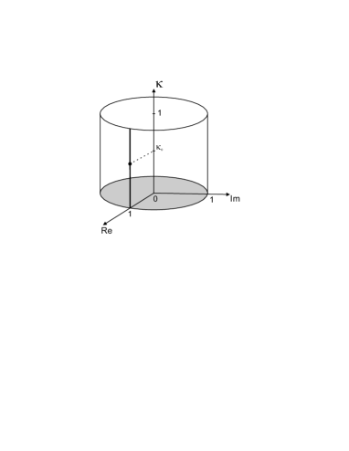
Figure 1. Parametric region $0\leq\kappa<1$, $0\leq\beta<\pi$

Theorem 14.

Let $V(z)$ belong to the generalized Donoghue class ${\mathfrak{M}}_{\kappa}$, $0\leq\kappa<1$. Then $V(z)$ can be realized as the impedance function $V_{\Theta_{\kappa}}(z)$ of an L-system $\Theta_{\kappa}$ of the form (44) with the triple $(\dot{A},T,\hat{A})$ that satisfies Hypothesis 5 with $A=\hat{A}$, the quasi-kernel of ${\rm Re\,}{\mathbb{A}}$. Moreover,

(82) $$V(z)=V_{\Theta_{\kappa}}(z)=\frac{1-\kappa}{1+\kappa}\,M({\dot{A}},\hat{A})(z),\quad z\in{\mathbb{C}}_{+},$$

where $M({\dot{A}},\hat{A})(z)$ is the Weyl-Titchmarsh function associated with the pair $({\dot{A}},\hat{A})$.

Proof.

Since $V(z)\in{\mathfrak{M}}_{\kappa}$, then it admits the integral representation (32) with normalization condition (63) on the measure $\mu$. Set

$$c=\frac{1+\kappa}{1-\kappa}.$$

It follows directly from definitions of classes ${\mathfrak{M}}$ and ${\mathfrak{M}}_{\kappa}$ that the function $cV\in{\mathfrak{M}}$ and thus has the integral representation (32) with the measure $\mu_{0}=c\mu$ and normalization condition (33) on the measure $\mu_{0}$. We use the measure $\mu_{0}$ to construct a model triple $(\dot{\mathcal{B}},T_{{\mathcal{B}}_{0}},{\mathcal{B}})$ described by (41)-(43) with $S(i)=0$. Note that the model triple $(\dot{\mathcal{B}},T_{{\mathcal{B}}_{0}},{\mathcal{B}})$ satisfies Hypothesis 5. Then we follow Step 1 of the proof of Theorem 7 to build an L-system $\Theta_{0}$ given by (47). According to (56) $V_{\Theta_{0}}(z)=M(\dot{\mathcal{B}},{\mathcal{B}})(z)$. On the other hand, since $M(\dot{\mathcal{B}},{\mathcal{B}})(z)$ is the Weyl-Titchmarsh function associated with the pair $(\dot{\mathcal{B}},{\mathcal{B}})$, then it also admits a representation

$$M(\dot{\mathcal{B}},{\mathcal{B}})(z)=\int_{\mathbb{R}}\left(\frac{1}{\lambda-z}-\frac{\lambda}{1+\lambda^{2}}\right)d\mu_{0},\quad z\in{\mathbb{C}}_{+},$$

with the same measure $\mu_{0}$ as in the representation for $cV$. Therefore,

$$cV(z)=M(\dot{\mathcal{B}},{\mathcal{B}})(z)=V_{\Theta_{0}}(z),\quad z\in{\mathbb{C}}_{+},$$

or $V(z)=(1/c)V_{\Theta_{0}}(z)$. Then we proceed with Step 2 of the proof of Theorem 7 to construct an L-system $\Theta^{\prime}$ given by (59). It is shown in (60) that

(83) $$V_{\Theta^{\prime}}(z)=\frac{1-\kappa}{1+\kappa}\,M(\dot{\mathcal{B}},{\mathcal{B}})(z),\quad z\in{\mathbb{C}}_{+},$$

and hence

$$V_{\Theta^{\prime}}(z)=\frac{1-\kappa}{1+\kappa}\,M(\dot{\mathcal{B}},{\mathcal{B}})(z)=\frac{1-\kappa}{1+\kappa}\,cV(z)=V(z).$$

Therefore, we have constructed an L-system $\Theta_{\kappa}=\Theta^{\prime}$ such that $V(z)=V_{\Theta_{\kappa}}(z)$. The remaining part of (82) follows from (83). ∎

7. Examples

Example 1

Following [1] we consider the prime symmetric operator

(84) $${\dot{A}}x =i\frac{dx}{dt},\;\text{\rm{Dom}}({\dot{A}})=\left\{x(t)\,\Big{|}\,x(t)-\text{abs. cont.},x^{\prime}(t)\in L^{2}_{[0,\ell]},\,x(0)=x(\ell)=0\right\}.$$

Its (normalized) deficiency vectors of ${\dot{A}}$ are

(85) $$g_{+}=\frac{\sqrt{2}}{\sqrt{e^{2\ell}-1}}e^{t}\in{\mathfrak{N}}_{i},\qquad g_{-}=\frac{\sqrt{2}}{\sqrt{1-e^{-2\ell}}}e^{-t}\in{\mathfrak{N}}_{-i}.$$

If we set $C=\frac{\sqrt{2}}{\sqrt{e^{2\ell}-1}}$, then (85) can be re-written as

$$g_{+}=Ce^{t},\quad g_{-}=Ce^{\ell}e^{-t}.$$

Let

(86) $$Ax =i\frac{dx}{dt},\;\text{\rm{Dom}}(A)=\left\{x(t)\,\Big{|}\,x(t)-\text{abs. cont.},x^{\prime}(t)\in L^{2}_{[0,\ell]},\,x(0)=-x(\ell)\right\}.$$

be a self-adjoint extension of ${\dot{A}}$. Clearly, $g_{+}(0)-g_{-}(0)=C-Ce^{\ell}$ and $g_{+}(\ell)-g_{-}(\ell)=Ce^{\ell}-C$ and hence (34) is satisfied, i.e., $g_{+}-g_{-}\in\text{\rm{Dom}}(A)$.

Then the Livšic characteristic function $s(z)$ for the pair $({\dot{A}},A)$ ha stye form (see [1])

(87) $$s(z)=\frac{e^{\ell}-e^{-i\ell z}}{1-e^{\ell}e^{-i\ell z}}.$$

We introduce the operator

(88) $$Tx =i\frac{dx}{dt},\;\text{\rm{Dom}}(T)=\left\{x(t)\,\Big{|}\,x(t)-\text{abs. cont.},x^{\prime}(t)\in L^{2}_{[0,\ell]},\,x(0)=0\right\}.$$

By construction, $T$ is a dissipative extension of ${\dot{A}}$ parameterized by a von Neumann parameter $\kappa$. To find $\kappa$ we use (85) with (30) to obtain

(89) $$x(t)=Ce^{t}-\kappa\,Ce^{\ell}e^{-t}\in\text{\rm{Dom}}(T),\quad x(0)=0,$$

yielding

(90) $$\kappa=e^{-\ell}.$$

Obviously, the triple of operators $(\dot{A},T,A)$ satisfy the conditions of Hypothesis 5 since $|\kappa|=e^{-\ell}<1$. Therefore, we can use (38) to write out the characteristic function $S(z)$ for the triple $({\dot{A}},T,A)$

(91) $$S(z)=\frac{s(z)-\kappa}{\bar{\kappa}s(z)-1}=\frac{e^{\ell}-\kappa+e^{-i\ell z}(\kappa e^{\ell}-1)}{\bar{\kappa}e^{\ell}-1+e^{-i\ell z}(e^{\ell}-\bar{\kappa})},$$

and apply the value of $\kappa=e^{-\ell}$ to get

(92) $$S(z)=e^{i\ell z}.$$

Now we shall use the triple $({\dot{A}},T,A)$ for an L-system $\Theta$ that we about to construct. First, we note that by the direct check one gets

(93) $$T^{*}x =i\frac{dx}{dt},\;\text{\rm{Dom}}(T)=\left\{x(t)\,\Big{|}\,x(t)-\text{abs. cont.},x^{\prime}(t)\in L^{2}_{[0,\ell]},\,x(\ell)=0\right\}.$$

Following the steps of Example 7.6 of [3] we have

(94) $${\dot{A}}^{\ast}x =i\frac{dx}{dt},\;\text{\rm{Dom}}({\dot{A}}^{\ast}) =\left\{x(t)\,\Big{|}\,x(t)-\text{ abs. cont.},x^{\prime}(t)\in L^{2}_{[0,\ell]}\right\}.$$

Then ${\mathcal{H}}_{+}=\text{\rm{Dom}}({\dot{A}}^{\ast})=W^{1}_{2}$ is the Sobolev space with scalar product

(95) $$(x,y)_{+}=\int_{0}^{\ell}x(t)\overline{y(t)}\,dt+\int_{0}^{\ell}x^{\prime}(t)\overline{y^{\prime}(t)}\,dt.$$

Construct rigged Hilbert space $W^{1}_{2}\subset L^{2}_{[0,\ell]}\subset(W_{2}^{1})_{-}$ and consider operators

(96) $${\mathbb{A}}x=i\frac{dx}{dt}+ix(0)\left[\delta(t)-\delta(t-\ell)\right],\quad{\mathbb{A}}^{\ast}x=i\frac{dx}{dt}+ix(l)\left[\delta(t)-\delta(t-\ell)\right],$$

where $x(t)\in W_{2}^{1}$, $\delta(t)$, $\delta(t-\ell)$ are delta-functions and elements of $(W^{1}_{2})_{-}$ that generate functionals by the formulas $(x,\delta(t))=x(0)$ and $(x,\delta(t-\ell))=x(\ell)$. It is easy to see that ${\mathbb{A}}\supset T\supset{\dot{A}}$, ${\mathbb{A}}^{\ast}\supset T^{\ast}\supset{\dot{A}},$ and that

$${\rm Re\,}{\mathbb{A}}x=i\frac{dx}{dt}+\frac{i}{2}(x(0)+x(\ell))\left[\delta(t)-\delta(t-\ell)\right].$$

Clearly, ${\rm Re\,}{\mathbb{A}}$ has its quasi-kernel equal to $A$ in (86). Moreover,

$$\operatorname{Im}{\mathbb{A}}x=\left(\cdot,\frac{1}{\sqrt{2}}[\delta(t)-\delta(t-\ell)]\right)\frac{1}{\sqrt{2}}[\delta(t)-\delta(t-\ell)]=(\cdot,\chi)\chi,$$

where $\chi=\frac{1}{\sqrt{2}}[\delta(t)-\delta(t-\ell)]$. Now we can build

(97) $$\Theta=\begin{pmatrix}{\mathbb{A}}&K&1\\ &&\\ W_{2}^{1}\subset L^{2}_{[0,\ell]}\subset(W^{1}_{2})_{-}&{}&{\mathbb{C}}\end{pmatrix},$$

that is a minimal L-system with

(98) $$Kc =c\cdot\chi=c\cdot\frac{1}{\sqrt{2}}[\delta(t)-\delta(t-l)],\quad(c\in{\mathbb{C}}),$$

$$K^{\ast}x =(x,\chi)=\left(x,\frac{1}{\sqrt{2}}[\delta(t)-\delta(t-l)]\right)=\frac{1}{\sqrt{2}}[x(0)-x(l)],$$

and $x(t)\in W^{1}_{2}$. In order to find the transfer function of $\Theta$ we begin by evaluating the resolvent of operator $T$ in (88). Solving the linear differential equation of the first order with the initial condition from (88) yields

(99) $$R_{z}(T)f=(T-zI)^{-1}f=-ie^{-izt}\int_{0}^{t}f(s)e^{izs}\,ds,\quad f\in L^{2}_{[0,\ell]}.$$

Similarly, one finds that

(100) $$R_{z}(T^{*})f=(T^{*}-zI)^{-1}f=ie^{-izt}\int_{t}^{\ell}f(s)e^{izs}\,ds,\quad f\in L^{2}_{[0,\ell]}.$$

We need to extend $R_{z}(T)$ to $(W^{1}_{2})_{-}$ to apply it to the vector $g$. We can accomplish this via finding the values of $\hat{R}_{z}(T)\delta(t)$ and $\hat{R}_{z}(T)\delta(t-l)$ (here $\hat{R}_{z}(T)$ is the extended resolvent). We have

$$(\hat{R}_{z}(T)\delta(t),f) =(\delta(t),R_{\bar{z}}(T^{*})f)=\overline{R_{\bar{z}}(T^{*})f\Big{|}_{t=0}}={-i}\int_{0}^{\ell}e^{-izs}\overline{f(s)}ds$$

$$=(-ie^{-izt},f),\quad f\in L^{2}_{[0,\ell]},$$

and hence $\hat{R}_{z}(T)\delta(t)=-ie^{-izt}$. Similarly, we determine that $\hat{R}_{z}(T)\delta(t-l)=0$. Consequently,

$$\hat{R}_{z}(T)g=-\frac{i}{\sqrt{2}}e^{-izt}.$$

Therefore,

(101) $$W_{\Theta}(z) =1-2i((T-zI)^{-1}\chi,\chi)=1-2i\left(-\frac{i}{\sqrt{2}}e^{-izt},\frac{1}{\sqrt{2}}[\delta(t)-\delta(t-\ell)]\right)$$

$$=1-(e^{-izt},\delta(t)-\delta(t-\ell))=1-1+e^{-i\ell z}=e^{-i\ell z}.$$

This confirms the result of Theorem 7 and formula (55) by showing that $W_{\Theta}(z)=1/S(z)$. The corresponding impedance function is found via (8) and is

$$V_{\Theta}(z)=i\frac{e^{-i\ell z}-1}{e^{-i\ell z}+1}.$$

Direct substitution yields

$$V_{\Theta}(i)=i\frac{e^{\ell}-1}{e^{\ell}+1}=i\frac{1-e^{-\ell}}{1+e^{-\ell}}=i\frac{1-\kappa}{1+\kappa},$$

and thus $V_{\Theta}(z)\in{\mathfrak{M}}_{\kappa}$ with $\kappa=e^{-\ell}$.

Example 2

In this Example we will rely on the main elements of the construction presented in Example 1 but with some changes. Let ${\dot{A}}$ and $A$ be still defined by formulas (84) and (86), respectively and let $s(z)$ be the Livšic characteristic function $s(z)$ for the pair $({\dot{A}},A)$ given by (87). We introduce the operator

(102) $$T_{0}x=i\frac{dx}{dt},\;$$

$$\text{\rm{Dom}}(T_{0})=\left\{x(t)\,\Big{|}\,x(t)-\text{abs. cont.},x^{\prime}(t)\in L^{2}_{[0,\ell]},\,x(\ell)=e^{\ell}x(0)\right\}.$$

It turns out that $T_{0}$ is a dissipative extension of ${\dot{A}}$ parameterized by a von Neumann parameter $\kappa=0$. Indeed, using (85) with (30) again we obtain

(103) $$x(t)=Ce^{t}-\kappa\,Ce^{\ell}e^{-t}\in\text{\rm{Dom}}(T),\quad x(\ell)=e^{\ell}x(0),$$

yielding $\kappa=0$. Clearly, the triple of operators $(\dot{A},T_{0},A)$ satisfy the conditions of Hypothesis 5 but this time, since $\kappa=0$, we have that $S(z)=-s(z)$.

Following the steps of Example 1 we are going to use the triple $({\dot{A}},T_{0},A)$ in the construction of an L-system $\Theta_{0}$. By the direct check one gets

(104) $$T_{0}^{*}x=i\frac{dx}{dt},$$

$$\text{\rm{Dom}}(T)=\left\{x(t)\,\Big{|}\,x(t)-\text{abs. cont.},x^{\prime}(t)\in L^{2}_{[0,\ell]},\,x(\ell)=e^{-\ell}x(0)\right\}.$$

Once again, we have ${\dot{A}}^{*}$ defined by (94) and ${\mathcal{H}}_{+}=\text{\rm{Dom}}({\dot{A}}^{\ast})=W^{1}_{2}$ is a space with scalar product (95). Consider the operators

(105) $${\mathbb{A}}_{0}x =i\frac{dx}{dt}+i\frac{x(\ell)-e^{\ell}x(0)}{e^{\ell}-1}\left[\delta(t-\ell)-\delta(t)\right],$$

$${\mathbb{A}}_{0}^{\ast} x=i\frac{dx}{dt}+i\frac{x(0)-e^{\ell}x(\ell)}{e^{\ell}-1}\left[\delta(t-\ell)-\delta(t)\right],$$

where $x(t)\in W_{2}^{1}$. It is easy to see that ${\mathbb{A}}\supset T_{0}\supset{\dot{A}}$, ${\mathbb{A}}^{\ast}\supset T_{0}^{\ast}\supset{\dot{A}},$ and

$${\rm Re\,}{\mathbb{A}}_{0}x=i\frac{dx}{dt}-\frac{i}{2}(x(0)+x(\ell))\left[\delta(t-\ell)-\delta(t)\right].$$

Thus ${\rm Re\,}{\mathbb{A}}_{0}$ has its quasi-kernel equal to $A$ in (86). Similarly,

$$\operatorname{Im}{\mathbb{A}}_{0}x=\left(\frac{1}{2}\right)\frac{e^{\ell}+1}{e^{\ell}-1}(x(\ell)-x(0))\left[\delta(t-\ell)-\delta(t)\right].$$

Therefore,

$$\operatorname{Im}{\mathbb{A}}_{0} =\left(\cdot,\sqrt{\frac{e^{\ell}+1}{2(e^{\ell}-1)}}\,\left[\delta(t-\ell)-\delta(t)\right]\right)\sqrt{\frac{e^{\ell}+1}{2(e^{\ell}-1)}}\,\left[\delta(t-\ell)-\delta(t)\right]$$

$$=(\cdot,\chi_{0})\chi_{0},$$

where $\chi_{0}=\sqrt{\frac{e^{\ell}+1}{2(e^{\ell}-1)}}\,[\delta(t-\ell)-\delta(t)]$. Now we can build

$$\Theta_{0}=\begin{pmatrix}{\mathbb{A}}_{0}&K_{0}&1\\ &&\\ W_{2}^{1}\subset L^{2}_{[0,l]}\subset(W^{1}_{2})_{-}&{}&{\mathbb{C}}\end{pmatrix},$$

which is a minimal L-system with $K_{0}c=c\cdot\chi_{0}$, $(c\in{\mathbb{C}})$, $K_{0}^{\ast}x=(x,\chi_{0})$ and $x(t)\in W^{1}_{2}$. Following Example 1 we derive

(106) $$R_{z}(T_{0}) =(T_{0}-zI)^{-1}f$$

$$=-ie^{-izt}\left(\int_{0}^{t}f(s)e^{izs}\,ds+\frac{e^{-i\ell z}}{e^{\ell}-e^{-i\ell z}}\int_{0}^{l}f(s)e^{izs}\,ds\right),$$

and

(107) $$R_{z}(T_{0}^{*}) =(T_{0}^{*}-zI)^{-1}f$$

$$=-ie^{-izt}\left(\int_{0}^{t}f(s)e^{izs}\,ds+\frac{e^{-i\ell z}}{e^{-\ell}-e^{-i\ell z}}\int_{0}^{l}f(s)e^{izs}\,ds\right),$$

for $f\in L^{2}_{[0,\ell]}$. Then again

$$(\hat{R}_{z}(T_{0})\delta(t),f) =(\delta(t),R_{\bar{z}}(T_{0}^{*})f)=\overline{R_{\bar{z}}(T_{0}^{*})f\Big{|}_{t=0}}=\frac{ie^{i\ell z}}{e^{-\ell}-e^{i\ell z}}\int_{0}^{\ell}e^{-izs}\overline{f(s)}ds$$

$$=\frac{ie^{\ell}}{e^{-i\ell z}-e^{\ell}}(e^{-izt},f),\quad f\in L^{2}_{[0,\ell]}.$$

Similarly,

$$(\hat{R}_{z}(T_{0}) \delta(t-\ell),f)=(\delta(t-\ell),R_{\bar{z}}(T_{0}^{*})f)=\overline{R_{\bar{z}}(T_{0}^{*})f\Big{|}_{t=\ell}}$$

$$=\frac{ie^{i\ell z}e^{-\ell}}{e^{-\ell}-e^{i\ell z}}\int_{0}^{\ell}e^{-izs}\overline{f(s)}ds=\frac{i}{e^{-i\ell z}-e^{\ell}}(e^{-izt},f),\quad f\in L^{2}_{[0,\ell]}.$$

Hence,

(108) $$\hat{R}_{z}(T_{0})\delta(t)=\frac{ie^{\ell}}{e^{-i\ell z}-e^{\ell}}\,e^{-izt},\quad\hat{R}_{z}(T_{0})\delta(t-\ell)=\frac{i}{e^{-i\ell z}-e^{\ell}}\,e^{-izt},$$

and

$$\hat{R}_{z}(T_{0})\chi_{0}=\hat{R}_{z}(T_{0})\sqrt{\frac{e^{\ell}+1}{2(e^{\ell}-1)}}\left[\delta(t-\ell)-\delta(t)\right]=\sqrt{\frac{e^{\ell}+1}{2(e^{\ell}-1)}}\frac{i-ie^{\ell}}{e^{-i\ell z}-e^{\ell}}\,e^{-izt}.$$

Using techniques of Example 1 one finds the transfer function of $\Theta_{0}$ to be

$$W_{\Theta_{0}}(z) =1-2i(\hat{R}_{z}(T_{0})\chi_{0},\chi_{0})$$

$$=1-2i\left(\sqrt{\frac{e^{\ell}+1}{2(e^{\ell}-1)}}\frac{i-ie^{\ell}}{e^{-i\ell z}-e^{\ell}}\,e^{-izt},\sqrt{\frac{e^{\ell}+1}{2(e^{\ell}-1)}}[\delta(t-\ell)-\delta(t)]\right)$$

$$=1+\frac{e^{\ell}+1}{e^{\ell}-1}\left(\frac{e^{\ell}-1}{e^{-i\ell z}-e^{\ell}}\,e^{-izt},\delta(t-\ell)-\delta(t)\right)$$

$$=1-\frac{e^{\ell}+1}{e^{\ell}-1}\left(\frac{e^{\ell}-1}{e^{-i\ell z}-e^{\ell}}-\frac{(e^{\ell}-1)e^{-iz\ell}}{e^{-i\ell z}-e^{\ell}}\right)$$

$$=1+(e^{\ell}+1)\left(\frac{1-e^{-iz\ell}}{e^{-i\ell z}-e^{\ell}}\right)$$

$$=\frac{e^{\ell}e^{-i\ell z}-1}{e^{\ell}-e^{-i\ell z}}.$$

This confirms the result of Corollary 8 and formula (55) by showing that $W_{\Theta_{0}}(z)=-1/s(z)$. The corresponding impedance function is

$$V_{\Theta_{0}}(z)=i\frac{e^{\ell}+1}{e^{\ell}-1}\cdot\frac{e^{-i\ell z}-1}{e^{-i\ell z}+1}.$$

A quick inspection confirms that $V_{\Theta_{0}}(i)=i$ and hence $V_{\Theta_{0}}(z)\in{\mathfrak{M}}$.

Remark

We can use Examples 1 and 2 to illustrate Lemma 10 and Theorem 12. As one can easily tell that the impedance function $V_{\Theta_{0}}(z)$ from Example 2 above and the impedance function $V_{\Theta}(z)$ from Example 1 are related via (64) with $\kappa=e^{-\ell}$, that is,

$$V_{\Theta}(z)=\frac{1-e^{-\ell}}{1+e^{-\ell}}\,V_{\Theta_{0}}(z).$$

Let $\Theta$ be the L-system of the form (97) described in Example 1 with the transfer function $W_{\Theta}(z)$ given by (101). It was shown in [3, Theorem 8.3.1] that if one takes a function $W(z)=-W_{\Theta}(z)$, then $W(z)$ can be realized as a transfer function of another L-system $\Theta_{1}$ that shares the same main operator $T$ with $\Theta$ and in this case

$$V_{\Theta_{1}}(z)=-1/V_{\Theta}(z)=i\frac{e^{-i\ell z}+1}{e^{-i\ell z}-1}.$$

Clearly, $V_{\Theta_{1}}(z)$ and $V_{\Theta_{0}}(z)$ are not related via (64) even though $\Theta_{1}$ has the same operator $T$ with the same parameter $\kappa=e^{-\ell}$ as in $\Theta$. The reason for that is the fact that the quasi-kernel of the real part of ${\mathbb{A}}_{1}$ of the L-system $\Theta_{1}$ does not satisfy the conditions of Hypothesis 5 as indicated by Theorem 12.

Example 3

In this Example we are going to extend the construction of Example 2 to obtain a family of L-systems $\Theta_{0}(\beta)$ described in (73). Let ${\dot{A}}$ be defined by formula (84) but the operator $A$ be an arbitrary self-adjoint extension of ${\dot{A}}$. It is known then [1] that all such operators $A$ are described with the help of a unimodular parameter $\mu$ as follows

(109) $$Ax =i\frac{dx}{dt},$$

$$\text{\rm{Dom}}(A) =\left\{x(t)\,\Big{|}\,x(t)\in\text{\rm{Dom}}({\dot{A}}^{*}),\,\mu x(\ell)+x(0)=0,\,|\mu|=1\right\}.$$

In order to establish the connection between the boundary value $\mu$ in (109) and the von Neumann parameter $U$ in (4) we follow the steps similar to Example 1 to guarantee that $g_{+}+Ug_{-}\in\text{\rm{Dom}}(A)$, where $g_{\pm}$ are given by (85). Quick set of calculations yields

(110) $$U=-\frac{1+\mu e^{\ell}}{\mu+e^{\ell}}.$$

For this value of $U$ we set the value of $\beta$ so that $U=e^{2i\beta}$, where $\beta\in[0,\pi)$ and thus establish the link between the parameters $\mu$ and $\beta$ that will be used to construct the family $\Theta_{0}(\beta)$. In particular, we note that $\beta=0$ if and only if $\mu=-1$.

Once again, having ${\dot{A}}^{*}$ defined by (94) and ${\mathcal{H}}_{+}=\text{\rm{Dom}}({\dot{A}}^{\ast})=W^{1}_{2}$ a space with scalar product (95), consider the following operators

(111) $${\mathbb{A}}_{0}(\beta)x =i\frac{dx}{dt}+i\frac{\bar{\mu}}{\bar{\mu}+e^{-\ell}}(x(0)-e^{-\ell}x(\ell))\left[\mu\delta(t-\ell)+\delta(t)\right],$$

$${\mathbb{A}}_{0}^{\ast}(\beta) x=i\frac{dx}{dt}+i\frac{1}{\mu+e^{-\ell}}(e^{-\ell}x(0)-x(\ell))\left[\mu\delta(t-\ell)+\delta(t)\right],$$

where $x(t)\in W_{2}^{1}$. It is immediate that ${\mathbb{A}}\supset T_{0}\supset{\dot{A}}$, ${\mathbb{A}}^{\ast}\supset T_{0}^{\ast}\supset{\dot{A}},$ where $T_{0}$ and $T_{0}^{*}$ are given by (102) and (104). Also, as one can easily see, when $\beta=0$ and consequently $\mu=-1$, the operators ${\mathbb{A}}_{0}(0)$ and ${\mathbb{A}}_{0}^{\ast}(0)$ in (111) match the corresponding pair ${\mathbb{A}}_{0}$ and ${\mathbb{A}}_{0}^{*}$ in (105). By performing direct calculations we obtain

$${\rm Re\,}{\mathbb{A}}_{0}(\beta)x=i\frac{dx}{dt}+\frac{i}{2}(\nu x(\ell)+x(0))\left[\mu\delta(t-\ell)+\delta(t)\right],$$

where

(112) $$\nu=\frac{2\mu e^{-\ell}+e^{-2\ell}+1}{\mu+2e^{-\ell}+\mu e^{-2\ell}},$$

and $|\nu|=1.$ Consequently, ${\rm Re\,}{\mathbb{A}}_{0}$ has its quasi-kernel

(113) $$\hat{A}_{0}(\beta)=i\frac{dx}{dt},\quad\text{\rm{Dom}}(A)=\left\{x(t)\,\Big{|}\,x(t)\in\text{\rm{Dom}}({\dot{A}}^{*}),\,\nu x(\ell)+x(0)=0\right\}.$$

Moreover,

$$\operatorname{Im}{\mathbb{A}}_{0}(\beta)x=\left(\frac{1}{2}\right)\left(\frac{1-e^{-2\ell}}{|\mu+e^{-2\ell}|}\right)(\bar{\mu}x(\ell)+x(0))\left[\mu\delta(t-\ell)+\delta(t)\right].$$

Therefore,

$$\operatorname{Im}{\mathbb{A}}_{0}(\beta) =\left(\cdot,\frac{\sqrt{1-e^{-2\ell}}}{\sqrt{2}|\mu+e^{-2\ell}|}\,\left[\mu\delta(t-\ell)+\delta(t)\right]\right)\frac{\sqrt{1-e^{-2\ell}}}{\sqrt{2}|\mu+e^{-2\ell}|}\,\left[\mu\delta(t-\ell)+\delta(t)\right]$$

$$=(\cdot,\chi_{0}(\beta))\chi_{0}(\beta),$$

where $\chi_{0}(\beta)=\sqrt{\frac{e^{\ell}+1}{2(e^{\ell}-1)}}\,[\delta(t-\ell)-\delta(t)]$. Now we can compose our one-parametric L-system family

$$\Theta_{0}(\beta)=\begin{pmatrix}{\mathbb{A}}_{0}(\beta)&K_{0}(\beta)&1\\ &&\\ W_{2}^{1}\subset L^{2}_{[0,l]}\subset(W^{1}_{2})_{-}&{}&{\mathbb{C}}\end{pmatrix},$$

where $K_{0}(\beta)c=c\cdot\chi_{0}(\beta)$, $(c\in{\mathbb{C}})$, $K_{0}^{\ast}(\beta)x=(x,\chi_{0}(\beta))$ and $x(t)\in W^{1}_{2}$. Using techniques of Example 2 one finds the transfer function of $\Theta_{0}(\beta)$ to be

$$W_{\Theta_{0}(\beta)}(z) =1-2i(\hat{R}_{z}(T_{0})\chi_{0}(\beta),\chi_{0}(\beta))=\left(\frac{e^{\ell}+\mu}{\mu e^{\ell}+1}\right)\frac{e^{\ell}e^{-i\ell z}-1}{e^{\ell}-e^{-i\ell z}}.$$

The corresponding impedance function is again found via (8)

$$V_{\Theta_{0}(\beta)}(z)=i\frac{(\bar{\mu}e^{-i\ell z}-1)(e^{2\ell}+1)+2e^{\ell}e^{-i\ell z}-2\bar{\mu}e^{\ell}}{(\bar{\mu}e^{-i\ell z}+1)(e^{2\ell}-1)}.$$

A quick inspection confirms that $V_{\Theta_{0}(\beta)}(i)=i$ and hence $V_{\Theta_{0}(\beta)}(z)$ belongs to the Donoghue class ${\mathfrak{M}}$ for all $\beta\in[0,\pi)$ (equivalently $|\mu|=1$). Also, one can see that if $\beta=0$ and consequently $\mu=-1$ the conditions of Hypothesis 5 are satisfied and the L-system $\Theta_{0}(0)$ coincides with the L-system $\Theta_{0}$ of Example 2 and so do its transfer and impedance functions.

Example 4

In this Example we will generalize the results obtained in Examples 1 and 2. Once again, let ${\dot{A}}$ and $A$ be defined by formulas (84) and (86), respectively and let $s(z)$ be the Livšic characteristic function $s(z)$ for the pair $({\dot{A}},A)$ given by (87). We introduce a one-parametric family of operators

(114) $$T_{\rho}x =i\frac{dx}{dt},\;\text{\rm{Dom}}(T_{\rho})=\left\{x(t)\,\Big{|}\,x(t)-\text{abs. cont.},x^{\prime}(t)\in L^{2}_{[0,\ell]},\,x(\ell)=\rho x(0)\right\}.$$

We are going to select the values of boundary parameter $\rho$ in a way that will make $T_{\rho}$ compliant with Hypothesis 5. By performing the direct check we conclude that $\operatorname{Im}(T_{\rho}f,f)\geq 0$ for $f\in\text{\rm{Dom}}(T_{\rho})$ if $|\rho|>1$. This will guarantee that $T_{\rho}$ is a dissipative extension of ${\dot{A}}$ parameterized by a von Neumann parameter $\kappa$. For further convenience we assume that $\rho\in{\mathbb{R}}$. To find the connection between $\kappa$ and $\rho$ we use (85) with (30) again to obtain

(115) $$x(t)=Ce^{t}-\kappa\,Ce^{\ell}e^{-t}\in\text{\rm{Dom}}(T),\quad x(\ell)=\rho x(0).$$

Solving (115) in two ways yields

(116) $$\kappa=\frac{\rho-e^{\ell}}{\rho e^{\ell}-1}\quad\textrm{ and }\quad\rho=\frac{\kappa-e^{\ell}}{\kappa e^{\ell}-1}.$$

Using the first of relations (116) to find which values of $\rho$ provide us with $0\leq\kappa<1$ we obtain

(117) $$\rho\in(-\infty,-1)\cup[e^{\ell},+\infty).$$

Now assuming (117) we can acknowledge that the triplet of operators $(\dot{A},T_{\rho},A)$ satisfy the conditions of Hypothesis 5. Following Examples 1 and 2, we are going to use the triplet $({\dot{A}},T_{\rho},A)$ in the construction of an L-system $\Theta_{\rho}$. By the direct check we have

(118) $$T_{\rho}^{*}x=i\frac{dx}{dt},$$

$$\text{\rm{Dom}}(T_{\rho})=\left\{x(t)\,\Big{|}\,x(t)-\text{abs. cont.},x^{\prime}(t)\in L^{2}_{[0,\ell]},\,\rho x(\ell)=x(0)\right\}.$$

Once again, we have ${\dot{A}}^{*}$ defined by (94) and ${\mathcal{H}}_{+}=\text{\rm{Dom}}({\dot{A}}^{\ast})=W^{1}_{2}$ is a space with scalar product (95). Consider the operators

(119) $${\mathbb{A}}_{\rho}x =i\frac{dx}{dt}+i\frac{x(\ell)-\rho x(0)}{\rho-1}\left[\delta(t-\ell)-\delta(t)\right],$$

$${\mathbb{A}}_{\rho}^{\ast} x=i\frac{dx}{dt}+i\frac{x(0)-\rho x(\ell)}{\rho-1}\left[\delta(t-\ell)-\delta(t)\right],$$

where $x(t)\in W_{2}^{1}$. One easily checks that since $\operatorname{Im}\rho=0$, then ${\mathbb{A}}_{\rho}^{*}$ is the adjoint to ${\mathbb{A}}_{\rho}$ operator. Evidently, that ${\mathbb{A}}\supset T_{\rho}\supset{\dot{A}}$, ${\mathbb{A}}^{\ast}\supset T_{\rho}^{\ast}\supset{\dot{A}},$ and

$${\rm Re\,}{\mathbb{A}}_{\rho}x=i\frac{dx}{dt}-\frac{i}{2}(x(0)+x(\ell))\left[\delta(t-\ell)-\delta(t)\right].$$

Thus ${\rm Re\,}{\mathbb{A}}_{\rho}$ has its quasi-kernel equal to $A$ defined in (86). Similarly,

$$\operatorname{Im}{\mathbb{A}}_{\rho}x=\left(\frac{1}{2}\right)\frac{\rho+1}{\rho-1}(x(\ell)-x(0))\left[\delta(t-\ell)-\delta(t)\right].$$

Therefore,

$$\operatorname{Im}{\mathbb{A}}_{\rho} =\left(\cdot,\sqrt{\frac{\rho+1}{2(\rho-1)}}\,\left[\delta(t-\ell)-\delta(t)\right]\right)\sqrt{\frac{\rho+1}{2(\rho-1)}}\,\left[\delta(t-\ell)-\delta(t)\right]$$

$$=(\cdot,\chi_{\rho})\chi_{\rho},$$

where $\chi_{\rho}=\sqrt{\frac{\rho+1}{2(\rho-1)}}\,[\delta(t-\ell)-\delta(t)]$. Now we can build

$$\Theta_{\rho}=\begin{pmatrix}{\mathbb{A}}_{\rho}&K_{\rho}&1\\ &&\\ W_{2}^{1}\subset L^{2}_{[0,l]}\subset(W^{1}_{2})_{-}&{}&{\mathbb{C}}\end{pmatrix},$$

which is a minimal L-system with $K_{\rho}c=c\cdot\chi_{\rho}$, $(c\in{\mathbb{C}})$, $K_{\rho}^{\ast}x=(x,\chi_{\rho})$ and $x(t)\in W^{1}_{2}$. Evaluating the transfer function $W_{\Theta_{\rho}}(z)$ resembles the steps performed in Example 2. We have

(120) $$R_{z}(T_{\rho}) =(T_{\rho}-zI)^{-1}f$$

$$=-ie^{-izt}\left(\int_{0}^{t}f(s)e^{izs}\,ds+\frac{e^{-i\ell z}}{\rho-e^{-i\ell z}}\int_{0}^{l}f(s)e^{izs}\,ds\right).$$

This leads to

$$\hat{R}_{z}(T_{\rho})\chi_{\rho}=\hat{R}_{z}(T_{\rho})\sqrt{\frac{\rho+1}{2(\rho-1)}}\left[\delta(t-\ell)-\delta(t)\right]=i\sqrt{\frac{\rho+1}{2(\rho-1)}}\left(\frac{1-\rho}{e^{-i\ell z}-\rho}\right)\,e^{-izt},$$

and eventually to

$$W_{\Theta_{\rho}}(z)=1-2i(\hat{R}_{z}(T_{\rho})\chi_{\rho},\chi_{\rho})=\frac{\rho e^{-i\ell z}-1}{\rho-e^{-i\ell z}}.$$

Evaluating the impedance function $V_{\Theta_{\rho}}(z)$ results in

$$V_{\Theta_{\rho}}(z)=i\frac{\rho+1}{\rho-1}\cdot\frac{1-e^{-i\ell z}}{1+e^{-i\ell z}}.$$

Using direct calculations and (116) gives us

$$\frac{\rho+1}{\rho-1}=\frac{1-\kappa}{1+\kappa}\cdot\frac{e^{\ell}+1}{e^{\ell}-1},$$

and thus

$$V_{\Theta_{\rho}}(z)=\frac{1-\kappa}{1+\kappa}\,V_{\Theta_{0}}(z),$$

which confirms the result of Lemma 10.

Appendix A Rigged Hilbert spaces

In this Appendix we are going to explain the construction and basic geometry of rigged Hilbert spaces.

We start with a Hilbert space $\mathcal{H}$ with inner product $(x,y)$ and norm $\|\cdot\|$. Let $\mathcal{H}_{+}$ be a dense in ${\mathcal{H}}$ linear set that is a Hilbert space itself with respect to another inner product $(x,y)_{+}$ generating the norm $\|\cdot\|_{+}$. We assume that $\|x\|\leq\|x\|_{+}$, ($x\in{\mathcal{H}}_{+}$), i.e., the norm $\|\cdot\|_{+}$ generates a stronger than $\|\cdot\|$ topology in ${\mathcal{H}}_{+}$. The space $\mathcal{H}_{+}$ is called the space with the positive norm.

Now let $\mathcal{H}_{-}$ be a space dual to $\mathcal{H}_{+}$. It means that $\mathcal{H}_{-}$ is a space of linear functionals defined on $\mathcal{H}_{+}$ and continuous with respect to $\|\cdot\|_{+}$. By the $\|\cdot\|_{-}$ we denote the norm in $\mathcal{H}_{-}$ that has a form

$$\|h\|_{-}=\sup\limits_{u\in{\mathcal{H}}_{+}}\frac{|(h,u)|}{\|u\|_{+}},\;h\in{\mathcal{H}}.$$

The value of a functional $f\in\mathcal{H}_{-}$ on a vector $u\in\mathcal{H}_{+}$ is denoted by $(u,f)$. The space $\mathcal{H}_{-}$ is called the space with the negative norm.

Consider an embedding operator $\sigma:{\mathcal{H}}_{+}\mapsto{\mathcal{H}}$ that embeds ${\mathcal{H}}_{+}$ into ${\mathcal{H}}$. Since $\|\sigma f\|\leq\|f\|_{+}$ for all $f\in{\mathcal{H}}_{+}$, then $\sigma\in[{\mathcal{H}}_{+},{\mathcal{H}}]$. The adjoint operator $\sigma^{*}$ maps ${\mathcal{H}}$ into ${\mathcal{H}}_{-}$ and satisfies the condition $\|\sigma^{*}f\|_{-}\leq\|f\|$ for all $f\in{\mathcal{H}}$. Since $\sigma$ is a monomorphism with a $(\cdot)$-dense range, then $\sigma^{*}$ is a monomorphism with $(-)$-dense range. By identifying $\sigma^{*}f$ with $f$ ($f\in{\mathcal{H}}$) we can consider ${\mathcal{H}}$ embedded in ${\mathcal{H}}_{-}$ as a $(-)$-dense set and $\|f\|_{-}\leq\|f\|$. Also, the relation

$$(\sigma f,h)=(f,\sigma^{*}h),\qquad f\in{\mathcal{H}}_{+},\,h\in{\mathcal{H}},$$

implies that the value of the functional $\sigma^{*}h\in{\mathcal{H}}$ calculated at a vector $f\in{\mathcal{H}}_{+}$ as $(f,\sigma^{*}h)$ corresponds to the value $(f,h)$ in the space ${\mathcal{H}}$.

It follows from the Riesz representation theorem that there exists an isometric operator ${\mathcal{R}}$ which maps $\mathcal{H}_{-}$ onto $\mathcal{H}_{+}$ such that $(f,g)=(f,{\mathcal{R}}g)_{+}$ ($\forall f\in{\mathcal{H}}_{+}$, $g\in{\mathcal{H}}_{-}$) and $\|{\mathcal{R}}g\|_{+}=\|g\|_{-}$. Now we can turn ${\mathcal{H}}_{-}$ into a Hilbert space by introducing $(f,g)_{-}=({\mathcal{R}}f,{\mathcal{R}}g)_{+}$. Thus,

(121) $$(f,g)_{-}=(f,{\mathcal{R}}g)=({\mathcal{R}}f,g)=({\mathcal{R}}f,{\mathcal{R}}g)_{+},\qquad(f,g\in\mathcal{H}_{-}),$$

$$(u,v)_{+}=(u,{\mathcal{R}}^{-1}v)=({\mathcal{R}}^{-1}u,v)=({\mathcal{R}}^{-1}u,{\mathcal{R}}^{-1}v)_{-},\qquad(u,v\in\mathcal{H}_{+}).$$

The operator ${\mathcal{R}}$ (or ${\mathcal{R}}^{-1}$) will be called the Riesz-Berezansky operator. We note that ${\mathcal{H}}_{+}$ is also dual to ${\mathcal{H}}_{-}$. Applying the above reasoning, we define a triplet $\mathcal{H}_{+}\subset\mathcal{H}\subset\mathcal{H}_{-}$ to be called the rigged Hilbert space [6], [7].

Now we explain how to construct a rigged Hilbert space using a symmetric operator. Let ${\dot{A}}$ be a closed symmetric operator whose domain $\text{\rm{Dom}}({\dot{A}})$ is not assumed to be dense in ${\mathcal{H}}$. Setting $\overline{\text{\rm{Dom}}({\dot{A}})}={\mathcal{H}}_{0}$, we can consider ${\dot{A}}$ as a densely defined operator from ${\mathcal{H}}_{0}$ into ${\mathcal{H}}$. Clearly, $\text{\rm{Dom}}({\dot{A}}^{*})$ is dense in ${\mathcal{H}}$ and $\text{\rm{Ran}}({\dot{A}}^{*})\subset{\mathcal{H}}_{0}$. We introduce a new Hilbert space $\mathcal{H}_{+}=\text{\rm{Dom}}(\dot{A}^{*})$ with inner product

(122) $$(f,g)_{+}=(f,g)+(\dot{A}^{*}f,\dot{A}^{*}g),\qquad(f,g\in\mathcal{H}_{+}),$$

and then construct the operator generated rigged Hilbert space $\mathcal{H}_{+}\subset\mathcal{H}\subset\mathcal{H}_{-}$.

References

• [1] N. I. Akhiezer, I. M. Glazman, Theory of linear operators. Pitman Advanced Publishing Program, 1981.
• [2] A.  Aleman, R. T. W. Martin, W. T.  Ross, On a theorem of Livšic, J. Funct. Anal., 264, 999–1048, (2013).
• [3] Yu. Arlinskiĭ, S. Belyi, E. Tsekanovskiĭ, Conservative Realizations of Herglotz-Nevanlinna functions. Operator Theory: Advances and Applications, Vol. 217, Birkhäuser, 2011.
• [4] Yu. Arlinskiĭ, E. Tsekanovskiĭ, Constant $J$-unitary factor and operator-valued transfer functions. In: Dynamical systems and differential equations, Discrete Contin. Dyn. Syst., Wilmington, NC, 48–56, (2003).
• [5] S. Belyi, E. Tsekanovskiĭ, Realization theorems for operator-valued $R$-functions, Oper. Theory Adv. Appl., 98, 55–91, (1997).
• [6] Yu. M. Berezansky, Spaces with negative norm, Uspehi Mat. Nauk, vol. 18, no. 1 (109) 63–96, (1963) (Russian).
• [7] Yu. M. Berezansky, Expansion in eigenfunctions of self-adjoint operators, vol. 17, Transl. Math. Monographs, AMS, Providence, 1968.
• [8] M. S. Brodskii, Triangular and Jordan representations of linear operators. Translations of Mathematical Monographs, Vol. 32. American Mathematical Society, Providence, R.I., 1971.
• [9] M. S. Brodskii, M. S. Livšic, Spectral analysis of non-self-adjoint operators and intermediate systems, Uspehi Mat. Nauk (N.S.) 13, no. 1 (79), 3–85, (1958) (Russian).
• [10] V. A. Derkach, M. M. Malamud, Generalized resolvents and the boundary value problems for Hermitian operators with gaps, J. Funct. Anal. 95, 1–95, (1991).
• [11] W. F. Donoghue, On perturbation of spectra, Commun. Pure and Appl. Math. 18, 559–579, (1965).
• [12] F. Gesztesy, K. A. Makarov, E. Tsekanovskii, An addendum to Krein’s formula, J. Math. Anal. Appl. 222, 594–606, (1998).
• [13] F. Gesztesy, E. Tsekanovskii, On Matrix-Valued Herglotz Functions, Math. Nachr. 218, 61–138, (2000).
• [14] A. N. Kochubei, Characteristic functions of symmetric operators and their extensions, Izv. Akad. Nauk Armyan. SSR Ser. Mat. 15, no. 3, 219–232, (1980) (Russian).
• [15] M. S. Livšic, On a class of linear operators in Hilbert space, Mat. Sbornik (2), 19, 239–262 (1946) (Russian); English transl.: Amer. Math. Soc. Transl., (2), 13, 61–83, (1960).
• [16] M. S. Livšic, On spectral decomposition of linear non-self-adjoint operators, Mat. Sbornik (76) 34, 145–198, (1954) (Russian); English transl.: Amer. Math. Soc. Transl. (2) 5, 67–114, (1957).
• [17] M. S. Livšic, Operators, oscillations, waves. Moscow, Nauka, 1966 (Russian); English transl.: Amer. Math. Soc. Transl., Vol. 34., Providence, R.I., (1973).
• [18] K. A.  Makarov, E. Tsekanovskiĭ, On the Weyl-Titchmarsh and Livšic functions, Proceedings of Symposia in Pure Mathematics, Vol. 87, 291–313, American Mathematical Society, (2013).
• [19] K. A.  Makarov, E. Tsekanovskiĭ, On the addition and multiplication theorems, Operator Theory: Advances and Applications, 244, 315–339, (2015).
• [20] M. A. Naimark, Linear Differential Operators II., F. Ungar Publ., New York, 1968.
• [21] A. V. Shtraus, On the extensions and the characteristic function of a symmetric operator, Izv. Akad. Nauk SSR, Ser. Mat., 32, 186–207, (1968).
• [22] E. Tsekanovskiĭ, The description and the uniqueness of generalized extensions of quasi-Hermitian operators. (Russian) Funkcional. Anal. i Prilozen., 3, No.1, 95–96, (1969).
• [23] E. Tsekanovskiĭ,  Yu.  S̆muljan, The theory of bi-extensions of operators on rigged Hilbert spaces. Unbounded operator colligations and characteristic functions, Russ. Math. Surv., 32, 73–131, (1977).