Manipulation of gap nodes by uniaxial strain in iron-based superconductors

Abstract

In the iron pnictides and chalcogenides, multiple orbitals participate in the superconducting state, enabling different gap structures to be realized in distinct materials. Here we argue that the spectral weights of these orbitals can in principle be controlled by a tetragonal symmetry-breaking uniaxial strain, due to the enhanced nematic susceptibility of many iron-based superconductors. By investigating multi-orbital microscopic models in the presence of orbital order, we show that not only $T_{c}$ can be enhanced, but pairs of accidental gap nodes can be annihilated and created in the Fermi surface by an increasing external strain. We explain our results as a mixture of nearly-degenerate superconducting states promoted by strain, and show that the annihilation and creation of nodes can be detected experimentally via anisotropic penetration depth measurements. Our results provide a promising framework to externally control the superconducting properties of iron-based materials.

A distinguishing feature of iron pnictides and chalcogenides LaOFeAs ; BaFe2As2 is the non-universality of their gap structures. Experimentally, nodeless superconducting (SC) gaps are observed in optimally doped $\mathrm{Ba_{1-x}K_{x}Fe_{2}As_{2}}$ DingARPES122K ; Shimojima_Kdoped and $\mathrm{Ba(Fe_{1-x}Co_{x})_{2}As_{2}}$ Prozorov122CoGap , as well as in the undoped material $\mathrm{LiFeAs}$ BorisenkoLi111Gap ; AllanLiFeAs , while gap nodes are reported in optimally doped $\mathrm{BaFe_{2}(As_{1-x}P_{x})_{2}}$ Matsuda122PNode ; FengPnode ; Pdoped_nodes , $\mathrm{Ba(Fe_{1-x}Ru_{x})_{2}As_{2}}$ Ru_doped_nodes , and in the parent compounds $\mathrm{FeSe}$ Xue11Node and $\mathrm{KFe_{2}As_{2}}$ MatsudaK122Node ; ShinK122Node ; TailleferK122Pairing . This diversity of behaviors opens up the interesting possibility of manipulating the superconducting ground state by tuning the appropriate external parameters. While this can be achieved empirically by mixing different types of doping, such as $\mathrm{Ba(Fe_{1-x}Co_{x})_{2}(As_{1-y}P_{y})_{2}}$ Johrendta122CoP , control of the SC state requires understanding the mechanisms responsible for this non-universality of the gap structure.

Theoretically, spin fluctuations have been widely proposed to cause pairing in iron pnictides and chalcogenides magnetic . In this model, the non-universal behavior of the gap structure stems from the multi-orbital character of these materials that arises due to the $3d^{6}$ configuration of Fe reviews_pairing . In fact, first-principle calculations GraserSDDeg and ARPES experiments DingARPESOrbital ; Shen122CoOO reveal that the disconnected pockets that form the Fermi surface of most pnictides contain significant spectral weight from the $d_{xz}$, $d_{yz}$, and $d_{xy}$ orbitals (see Fig. 1(a)). While a sign-changing $s^{+-}$ state is favored by pairing within the $d_{xz}$ and $d_{yz}$ orbitals of different pockets, a $d$-wave state is preferred by the $d_{xy}$ orbitals. Thus, not only the leading SC instability, but also the presence or absence of nodes, depends on the orbital content of the Fermi pockets Kuroki09 ; GraserSDDeg ; Chubukov09 . Such a near-degeneracy between different SC ground states, supported by theoretical CWu09 ; KemperNJP ; Graser10 ; Ikeda10 ; Wang10 ; Maiti11 ; Thomale11 ; Fernandes13 ; Kotliar13 and experimental results raman_mode1 ; raman_mode2 , is a distinguishing feature of the iron-based materials, since in most superconductors one SC state usually has a much lower energy than all the other ones.

Therefore, in this framework, the properties of the SC state of the iron pnictides could be manipulated if the orbital content of their Fermi surface could be tuned. In this paper, we propose that this can be achieved via application of uniaxial strain $\partial_{i}u_{i}$, where $\mathbf{u}$ denotes the displacement vector. Experimentally, many optimally-doped iron-based superconductors display a large nematic susceptibility $\chi_{\mathrm{nem}}$ FisherXnemDivergent ; Kuo13 ; shear_modulus ; Yoshizawa12 ; Matsuda12 ; Meingast122Xnem ; GallaisRamanNem ; Jigang14 ; PasupathyNa111NemAFM , implying that even a small uniaxial strain Fisher10 ; Tanatar10 ; Degiorgi12 ; Dhital12 can trigger a nematic state with sizable anisotropies in the lattice and, more interestingly, in the magnetic and orbital degrees of freedom RMFRevNem . While previous works investigated how superconductivity is affected by the nematic-induced anisotropy in the magnetic spectrum RMFSDMix , little is known about the impact of the induced anisotropy in the electronic spectrum. Indeed, in the nematic state, the onsite energies of the $d_{xz}$ and $d_{yz}$ orbitals become unequal, $\Delta_{oo}=\left\langle\varepsilon_{xz}\right\rangle-\left\langle\varepsilon_{yz}\right\rangle\neq 0$ Shen122CoOO ; Yi12 ; Zhang12 , affecting the orbital content of the Fermi surface w_ku10 ; Devereaux10 ; Phillips12 ; Kontani12 ; Dagotto13 ; Fernandes12 . Due to the large nematic susceptibility $\chi_{\mathrm{nem}}$, a sizeable orbital splitting $\Delta_{oo}\sim 50$ meV can be triggered even by a small uniaxial strain of the order of $10$ MPa Shen122CoOO ; Yi12 . Therefore, because of the sensitivity of the pairing state to the orbital content of the Fermi surface, strain can be a viable tuning parameter to manipulate the SC ground state.

Here, using a multi-orbital microscopic model, we show that by changing the $d_{xz}/d_{yz}$ orbital splitting via uniaxial strain $\Delta_{oo}\propto\left(\partial_{x}u_{x}-\partial_{y}u_{y}\right)\chi_{\mathrm{nem}}$, gap nodes can be created on a nodeless SC state or manipulated in a nodal SC state. Focusing on the latter case, we find that, as $\Delta_{oo}$ is enhanced, while pairs of accidental nodes are annihilated in the electron-like Fermi pockets, merging along the direction of the applied strain, pairs of nodes are created in the hole-like Fermi pockets, emerging along both $x$ and $y$ directions. Interestingly, an enhancement of $T_{c}$ accompanies the motion of the nodes. We argue that these behaviors are consistent with a sizable mixture between $s^{+-}$ and $d$-wave states promoted by orbital order, which is only meaningful because of the near-degeneracy between the two states. We also show that the annihilation and the creation of nodes can be detected experimentally by sharp features that arise in the penetration depth.

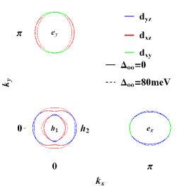
(a)

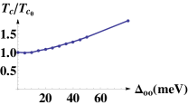
(b)

Figure 1: (a) Change of the FS by orbital order. The solid (dashed) lines describe the FS for $\Delta_{oo}=0$ ($\Delta_{oo}=80$ meV). Different colors represent the dominant $3d$ orbital component on the FS. (b) Enhancement of $T_{c}\propto\mathrm{e}^{-1/\lambda_{\alpha}}$ (in units of its value in the tetragonal phase $T_{c_{0}}$) as function of the orbital order parameter $\Delta_{oo}$.

Our starting point is the five-orbital Hubbard model with all possible on-site interactions KemperNJP ; reviews_pairing :

$$H= \sum_{ii^{\prime},ll^{\prime}}\sum_{\sigma}t_{il,i^{\prime}l^{\prime}}c_{il\sigma}^{\dagger}c_{i^{\prime}l^{\prime}\sigma}+U\sum_{i,l}n_{il\uparrow}n_{il\downarrow}$$ (1)

$$+U^{\prime}\sum_{i,l<l^{\prime}}n_{il}n_{il^{\prime}}+J\sum_{i,l<l^{\prime}}\sum_{\sigma,\sigma^{\prime}}c_{il\sigma}^{{\dagger}}c_{il^{\prime}\sigma^{\prime}}^{{\dagger}}c_{il\sigma^{\prime}}c_{il^{\prime}\sigma}$$

$$+J^{\prime}\sum_{il^{\prime}\neq l}c_{il\uparrow}^{{\dagger}}c_{il\downarrow}^{{\dagger}}c_{il^{\prime}\downarrow}c_{il^{\prime}\uparrow}+\frac{\Delta_{oo}}{2}\sum_{i}(n_{i,yz}-n_{i,xz})\ .$$

Here, $c_{il\sigma}^{\dagger}$ creates an electron at orbital $l$ and site $i$, and $n_{il\sigma}=c_{il\sigma}^{\dagger}c_{il\sigma}^{\phantom{\dagger}}$. The first term describes the band structure, with tight-binding parameters fitted to first-principle calculations (see Ref. KemperNJP for the hopping parameters). $U=1.3$ eV is the intra-orbital repulsion, $J=0.2$ eV is the Hund’s rule coupling, $J^{\prime}=J$ is the pair-hopping coupling, and $U^{\prime}=U-2J$ is the inter-orbital repulsion. The orbital order parameter $\Delta_{oo}$ gives the splitting between the $d_{xz}$ and $d_{yz}$ onsite energies. In the following, we consider that it is generated by uniaxial strain applied parallel to the $x$ direction, $\partial_{x}u_{x}>\partial_{y}u_{y}$, implying $\Delta_{oo}>0$ Shen122CoOO . Although strain also affects the onsite energies and hopping parameters of other orbitals, their impact on the electronic structure is small compared to the contribution arising from the $d_{xz}$-$d_{yz}$ orbital splitting Shen122CoOO .

The Fermi surface (FS) of this model for an occupation number $n\approx 6$ is displayed in Fig 1(a). In the tetragonal phase ($\Delta_{oo}=0$) the FS is composed of two $C_{4}$-symmetric central hole pockets ($h_{1}$, $h_{2}$) and two $C_{2}$-symmetric electron pockets ($e_{x}$, $e_{y}$) centered at $\left(\pi,0\right)$ and $\left(0,\pi\right)$. While $h_{1}$ and $h_{2}$ have only $d_{xz}$/$d_{yz}$ orbital character, $e_{x}$ has $d_{yz}/d_{xy}$ character and $e_{y}$, $d_{xz}/d_{xy}$ GraserSDDeg ; KemperNJP . Consequently, for a non-zero orbital order parameter $\Delta_{oo}$, the sizes of the two electron pockets become slightly different, and the two hole pockets are distorted into $C_{2}$-symmetric shapes Fernandes12 ; Lv11 . To investigate the effect of orbital order on SC, we solve numerically the linearized spin-fluctuation RPA gap equations KemperNJP ; reviews_pairing

$$-\sum_{j}\oint_{C_{j}}\frac{\mathrm{d}{\bf k}^{\prime}}{2\pi}\frac{1}{v_{F}({\bf k}^{\prime})}\Gamma^{ij}({\bf k},{\bf k}^{\prime})g_{\alpha j}({\bf k}^{\prime})=\lambda_{\alpha}g_{\alpha i}({\bf k})\ ,$$ (2)

where $v_{F}({\bf k})$ is the Fermi velocity, $C_{j}$ denotes one of the four Fermi pockets, and $\Gamma^{ij}({\bf k},{\bf k}^{\prime})$ is the effective pairing interaction which scatters a Cooper pair $({\bf k},-{\bf k})$ on the FS $C_{i}$ to $({\bf k}^{\prime},-{\bf k}^{\prime})$ on the FS $C_{j}$. The structure factor of the SC gap at pocket $C_{i}$ is given by $g_{\alpha i}\left(\mathbf{k}\right)$, and the largest eigenvalue $\lambda_{\alpha}$ gives the leading pairing instability, with $T_{c}\propto\mathrm{e}^{-1/\lambda_{\alpha}}$. For $\Delta_{oo}=0$, as shown previously GraserSDDeg ; KemperNJP , the leading pairing instability is the $s^{+-}$ state with accidental nodes on the two electron pockets (see red lines in Fig. 2), followed closely by a $d$-wave state with symmetry-constrained nodes along the diagonals of the Brillouin zone.

Solving the linearized gap equations in the presence of a non-zero orbital order $\Delta_{oo}\neq 0$ for a fixed occupation number, we find a steady enhancement of $T_{c}\propto\mathrm{e}^{-1/\lambda_{\alpha}}$ for increasing $\Delta_{oo}$, as shown in Fig. 1(b). The gap structure is also strongly affected by orbital order: in Fig. 2(a), we contrast the angular dependence of the gap around each of the Fermi pockets in the tetragonal phase ($\Delta_{oo}=0$) and in the presence of orbital order ($\Delta_{oo}=80$ meV, motivated by the experimentally measured values Shen122CoOO ; Yi12 ). Clearly, while in the $h_{1}$ and $h_{2}$ hole pockets the gaps become more anisotropic, in the $e_{x}$ and $e_{y}$ electron pockets they become more isotropic. Consequently, for increasing $\Delta_{oo}$, pairs of accidental gap nodes tend to be created in the hole pockets, emerging parallel (perpendicular) to the strain direction in $h_{1}$ ($h_{2}$), while the pairs of accidental nodes initially present in the electron pockets tend to be annihilated, merging along the strain direction for both $e_{x}$ and $e_{y}$. An schematic illustration of this nodal behavior is shown in Fig. 2(b).

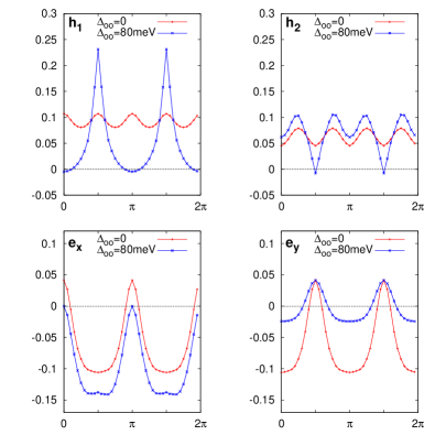
(a)

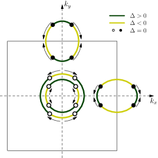
(b)

Figure 2: Evolution of gap structure at $T_{c}$ for increasing orbital order parameter $\Delta_{oo}$. The four panels in (a) show the angular dependencies of the gaps of each pocket in the presence (blue lines) and in the absence (red lines) of orbital order. The angles are measured relatively to the $x$ axis. (b) Schematic illustration of the motion of nodes as function of increasing $\Delta_{oo}$. While nodes are created in the hole pockets, emerging along both $x$ and $y$ directions (white dots), the electron pockets’ nodes are annihilated, merging along the $x$ direction (black dots). Green (yellow) lines denote positive (negative) gap values.

To show that these results are general and do not depend on details of the tight-binding model, we interpret them as a consequence of the mixing between the $s^{+-}$ and $d$-wave gap functions of the tetragonal state promoted by orbital order RMFSDMix :

$$\Delta\approx\Delta_{s}+\gamma\Delta_{d}\ ,$$ (3)

where $\gamma\propto\Delta_{oo}$ is the mixing parameter, which is sensitive to the applied strain and to the nematic susceptibility, since $\Delta_{\mathrm{oo}}\propto\left(\partial_{x}u_{x}-\partial_{y}u_{y}\right)\chi_{\mathrm{nem}}$. Of course, by symmetry, the gap function of any orthorhombic system is a mixture of $s$-wave and $d$-wave states. What makes the pnictides’ case interesting, and somehow unique, is the near-degeneracy between the $s^{+-}$ and $d$-wave states, which enforces the mixing parameter $\gamma$ to be sizable. This is to be contrasted to the case of orthorhombic cuprates, where the $s$-wave component arising from the orthorhombic symmetry is, for most purposes, irrelevant.

One of the consequences of the near-degeneracy between the competing $s^{+-}$ and $d$-wave states is the suppression of the value of $T_{c}$ in the tetragonal phase Fernandes13 ; RMFSDMix . The mixing between the two states promoted by orbital order, Eq. (3), lifts this degeneracy, which leads to an effective enhancement of $T_{c}$ Fernandes13 ; RMFSDMix , as found in Fig. 1(b). Interestingly, our RPA calculation suggests an enhancement that can be as large as $50\%$ for realistic values of $\Delta_{oo}$. Furthermore, Eq. (3) also explains qualitatively the motion of the gap nodes displayed in Fig. 2 as the natural evolution from a nodal $s^{+-}$ to a $d$-wave state. To illustrate this, consider simple harmonic expressions for the gaps in the tetragonal nodal $s^{+-}$ state, $\Delta_{h_{1/2}}^{(s)}=\Delta_{0}$ and $\Delta_{e_{x/y}}^{(s)}=-\Delta_{1}\pm\Delta_{2}\cos 2\phi_{x/y}$. Here, $\Delta_{j}>0$ and $\Delta_{2}>\Delta_{1}$; $\phi_{x/y}$ and $\theta$ denote the polar angles along the electron and hole pockets, respectively, measured with respect to the $x$ axis. The presence of orbital order gives rise to additional $d$-wave components $\Delta_{h_{1/2}}^{(d)}=\mp\tilde{\Delta}_{0}\cos 2\theta$ and $\Delta_{e_{x/y}}^{(d)}=\mp\tilde{\Delta}_{1}$ (with $\tilde{\Delta}_{j}>0$) in the gap functions. Thus, according to Eq. (3), as the mixing parameter $\gamma$ increases, the pairs of nodes initially present in the electron pockets eventually merge along the $x$ direction and disappear, while pairs of nodes appear in the hole pocket $h_{1}$ ($h_{2}$) along the $x$ ($y$) direction.

Whereas the above argument successfully accounts for the RPA calculations, a natural limitation of the latter is their validity only near $T_{c}$. An important question is whether the gap structure obtained at $T_{c}$ is robust down to $T=0$. To address this question, we developed an effective three-orbital model, inspired by the RPA analysis at $T_{c}$. In this model, only the $d_{xz}$, $d_{yz}$, and $d_{xy}$ orbitals are included, since their spectral weights dominate the FS (see Fig. 1). Furthermore, since the RPA-derived pairing interaction $\Gamma^{ij}({\bf k},{\bf k}^{\prime})$ is dominated by $i=h_{1}$ and $j=e_{x/y}$ KemperNJP , we consider these three pockets only. We also focus on the anisotropies introduced by the orbital contents of the FS pockets, rather than on their shapes. Consequently, we assume circular pockets and expand their wave-functions in terms of harmonic functions of their polar angles $\theta$ and $\phi_{x/y}$ (see also Refs. Maiti11 ; Vafek13 ):

$$\left|h\right\rangle=\cos\theta\left(1+\beta_{h}\sin^{2}\theta\right)\left|d_{xz}\right\rangle+\sin\theta\left(1-\beta_{h}\cos^{2}\theta\right)\left|d_{yz}\right\rangle$$

$$\left|e_{x/y}\right\rangle=\alpha\left|d_{xy}\right\rangle+\left(1\pm\beta_{e}\right)\left\{\begin{array}[]{c}\sin\phi_{x}\\ \cos\phi_{y}\end{array}\right\}\left|d_{yz/xz}\right\rangle$$ (6)

Here, the parameter $\alpha=0.52$ is obtained by fitting the angular dependence of $\left\langle\left.d_{a}\right|e_{x/y}\right\rangle$ to the corresponding tight-binding matrix elements for $\Delta_{oo}=0$ and the parameters $\beta_{h}$, $\beta_{e}=2\beta_{h}$ describe how the orbital weight around each pocket is changed by orbital order (see the supplementary material).

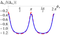
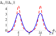
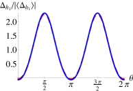
Figure 3: Angular dependence of the gaps on the hole ($h_{1}$) and electron ($e_{x/y}$) pockets at $T_{c}$ (dashed red line) and at $T=0$ (solid blue line) within our effective three-band model. The gaps are normalized by their absolute average values. The parameters used are: $v=0.30$, $w=0.25$, $\beta_{e}=2\beta_{h}=0.40$.

For the pairing interaction, motivated once again by the RPA results KemperNJP , we consider only the intra-orbital pairing interactions $v$ and $w$ connecting, respectively, the $d_{xz/yz}$ and $d_{xy}$ orbitals from different pockets. It is then straightforward to write down the BCS-like gap equations and solve them at any temperature (details in the supplementary material). For $\Delta_{oo}=0$ and at $T=T_{c}$, an $s^{+-}$ state with accidental nodes on the electron pockets is found for $v\gtrsim w$, whereas a $d$-wave state is found for $v\lesssim w$. To capture the near degeneracy between these two states, we focus on the regime $v\approx w$ – similar to the RPA case – and solve the gap equations for $T=0$ and $\Delta_{oo}\neq 0$. Fig. 3 contrasts the angular dependency of the gaps at $T=T_{c}$ and $T=0$, evidencing the robustness of the gap structure obtained at $T_{c}$. Furthermore, we also find that $T_{c}$ increases with increasing $\Delta_{oo}$, demonstrating that our effective model captures the RPA-derived results. An important issue is whether the $s$-$d$ mixing parameter $\gamma$ in Eq. 3 is always real, or whether imaginary solutions may arise, resulting in time-reversal symmetry-breaking states Valentin ; Maiti . Phenomenologically, the coupling between orbital order and SC gives rise to the quadratic free energy term $F\propto\Delta_{\mathrm{oo}}\left|\Delta_{s}\right|\left|\Delta_{d}\right|\cos\theta$, where $\theta$ is the relative phase between the SC order parameters, which is minimized by $\theta=0$ or $\theta=\pi$, i.e. by a real admixture of the $s^{+-}$ and d-wave states. In the supplementary material, we show explicitly that in our microscopic model $\Delta_{\mathrm{oo}}\neq 0$ favors a real $\gamma$ for all temperatures.

Having established that accidental nodes can be manipulated by uniaxial strain via the induced orbital order at all temperatures, we now discuss their experimental manifestations. As shown in Fig. 2, when pairs of nodes are annihilated (created) in the electron (hole) pockets, they merge into (emerge from) a single node with quadratic quasi-particle dispersion. These quadratic nodes give rise to a density of states $N\left(\omega\right)$ that scales as $\sqrt{\omega}$ at low energies quadratic_nodes1 ; quadratic_nodes2 ; quadratic_nodes3 – in contrast to the usual behavior for linear nodes $N\left(\omega\right)\sim\omega$ – strongly affecting the low-temperature behavior of thermodynamic quantities in the superconducting state.

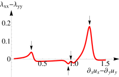
Figure 4: Anisotropic penetration depth, $\lambda_{xx}-\lambda_{yy}$, as a function of the mixing parameter $\gamma\propto\partial_{x}u_{x}-\partial_{y}u_{y}$ in Eq. (3), for $T/\Delta_{0}=0.01$. Arrows denote the peaks and troughs reflecting the annihilation and creation of nodes in the Fermi pockets.

This behavior is more clearly manifested in anisotropic quantities, such as the anisotropic penetration depth, $\lambda_{xx}-\lambda_{yy}$, which can be measured by tunnel diode resonators/oscillators and microwave cavities Matsuda_penetration_depth . Formally, it is given in terms of $\Delta\lambda_{\mu\mu}\propto-\int\mathrm{d}\omega\ \tilde{N}_{\mu\mu}(\omega)\frac{\partial f(\omega)}{\partial\omega}$, where $f(\omega)$ is the Fermi-Dirac distribution function,$\tilde{N}_{\mu\mu}(\omega)=\sum_{j}\int d^{2}k\ \delta(\omega-E_{j}({\bf k}))v_{j,\mu}^{F}v_{j,\mu}^{F}$ is the sum of the Fermi-velocity weighted density of states of all $j$ pockets, and $E_{j}({\bf k})$ is the corresponding quasi-particle dispersion. Analysis of this quantity reveals that, at low temperatures, the quadratic nodes only affect the component of the penetration depth parallel to the direction in which they appear or disappear, i.e. $\Delta\lambda_{\parallel}\propto\sqrt{T}$ whereas $\Delta\lambda_{\perp}\propto T$. As a result, $\lambda_{\parallel}\gg\lambda_{\perp}$ when a quadratic node appear or disappear from the Fermi surface, resulting in a peak or a trough in $\lambda_{xx}-\lambda_{yy}$. To illustrate this behavior, we plot in Fig. 4 $\lambda_{xx}-\lambda_{yy}$ as function of uniaxial strain, using Eq. (3) with $\gamma\propto\partial_{x}u_{x}-\partial_{y}u_{y}$, and $\Delta_{s}$ and $\Delta_{d}$ obtained from the solution of our effective model in Eq. (6) extended for four bands (see supplementary material). Two large peaks, corresponding to the annihilation of nodes in the electron pockets $e_{x}$ and $e_{y}$, are observed at small and large strain values, respectively. The peak resulting from the creation of nodes in the $h_{1}$ hole pocket nearly cancels the trough associated with the creation of nodes in $h_{2}$, as reflected by the weaker features in the intermediate strain region. Thus, $\lambda_{xx}-\lambda_{yy}$ is a viable quantity to probe the motion of nodes induced by uniaxial strain.

In summary, we showed that the multi-orbital character of the superconducting state of the iron pnictides, allied to the presence of a large nematic susceptibility, opens up the interesting possibility of enhancing $T_{c}$ and manipulating gap nodes by uniaxial strain. Our results rely on the proximity between the $s^{+-}$ and $d$-wave instabilities, as predicted by several theoretical models Kuroki09 ; KemperNJP ; Graser10 ; Ikeda10 ; Maiti11 ; Thomale11 and recently reported by Raman experiments in certain compounds raman_mode1 ; raman_mode2 . Our focus here was in systems that display accidental nodes already in the tetragonal phase, which is the case for $\mathrm{BaFe_{2}(As_{1-x}P_{x})_{2}}$ and possibly for $\mathrm{FeSe}$, $\mathrm{Ba(Fe_{1-x}Ru_{x})_{2}As_{2}}$ and $\mathrm{KFe_{2}As_{2}}$. Similar arguments imply that nodeless superconductors can be driven nodal by the application of uniaxial strain – in this case, however, nodes appear and disappear only in one of the electron pockets. Interestingly, quantum criticality has only been unambiguously detected in the nodal superconductor $\mathrm{BaFe_{2}(As_{1-x}P_{x})_{2}}$ Kasahara10 ; Matsuda_penetration_depth , which begs the question of whether nodal quasi-particles play a fundamental role in promoting this behavior. The possible manipulation of nodes by external strain may help shedding light on this important issue.

We thank C. Chen, A. Chubukov, H. Fu, S. Graser, P. Hirschfeld, T. Maier, S. Maiti, A. Millis, R. Prozorov, M. Tanatar, X. Wang, and V. Vakaryuk for helpful discussions.

Supplementary for “Manipulation of gap nodes by uniaxial strain in iron-based superconductors”

I Effective three band model

Our effective three band model contains the inner hole pocket $h_{1}$ and the two electron pockets $e_{x}$ and $e_{y}$. The outer hole pocket is ignored since the RPA-derived pairing interaction connecting $h_{2}$ to $e_{x/y}$ is weaker KemperNJP . As discussed in the main text, the (normalized) wave-function of the three Fermi surface pockets is expanded in harmonic functions of the angles around the pockets (measured with respect to the $x$ axis):

$$|h_{1}\rangle =\dfrac{\cos\theta(1+\beta_{h}\sin^{2}\theta)|d_{xz}\rangle+\sin\theta(1-\beta_{h}\cos^{2}\theta)|d_{yz}\rangle}{\left(1+\beta_{h}^{2}\sin^{2}\theta\cos^{2}\theta\right)^{1/2}}$$ (S1)

$$|e_{x}\rangle =\dfrac{\alpha|d_{xy}\rangle+(1+\beta_{e})\sin\phi_{x}|d_{yz}\rangle}{\left(\alpha^{2}+(1+\beta_{e})^{2}\sin^{2}\phi_{x}\right)^{1/2}}$$

$$|e_{y}\rangle =\dfrac{\alpha|d_{xy}\rangle+(1-\beta_{e})\cos\phi_{y}|d_{yz}\rangle}{\left(\alpha^{2}+(1-\beta_{e})^{2}\cos^{2}\phi_{y}\right)^{1/2}}\ ,$$

Here, $\alpha$ controls the angular dependence of the orbital weights on the electron pockets in the tetragonal phase, and $\beta_{h,e}$ describe the change in the orbital weights promoted by orbital order. To focus on the effects caused by the changes in orbital weight, and since the modification in the shapes of the Fermi pockets are small, we consider for simplicity three equal circular pockets. To obtain $\alpha$, we fit the matrix elements $\left\langle\left.d_{j}\right|e_{x}\right\rangle$ obtained from the equation above to those obtained from the tight-binding model. We find that $\alpha\approx 0.52$ yields a satisfactory description, as shown in Fig. S1.

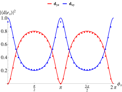
(a)

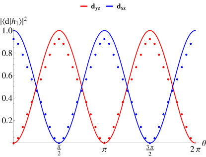
(b)

Figure S1: Orbital weight derived from the five orbital tight binding model (dots) and from the effective model, Eq. (S1), for $\alpha=0.52$. (a) $d_{xy}$ (blue) and $d_{yz}$ (red) orbital weights on the $e_{x}$ pocket. (b) $d_{yz}$ (red) and $d_{xz}$ (blue) orbital weights on the inner hole pocket $h_{1}$.

To obtain the pairing interaction in the band basis, we consider only the intra-orbital contributions:

$$\Gamma_{ij}\left(\mathbf{k},\mathbf{k}^{\prime}\right) =\sum_{i}\langle i|m\rangle_{\mathbf{k}}\langle i|m\rangle_{-\mathbf{k}}\ \Gamma_{mm}^{mm}\ \langle m|j\rangle_{\mathbf{k}^{\prime}}\langle m|j\rangle_{-\mathbf{k}^{\prime}}\ ,$$ (S2)

where $i$ and $j$ are band indices and $m$ is the orbital index. $\Gamma_{mm}^{mm}$ is the momentum independent pairing interaction in the orbital basis. Based on the RPA-derived pairing interaction, we consider only the intra-orbital pairing interactions connecting the same orbital on different pockets, $\Gamma_{mm}^{mm}=V$ for $m=d_{xz/yz}$ and $\Gamma_{mm}^{mm}=W$ for $m=d_{xy}$. Therefore:

$$\Gamma_{xy} =\dfrac{\alpha^{4}V}{\left(\alpha^{2}+(1+\beta_{e})^{2}\cos^{2}\phi_{x}\right)\left(\alpha^{2}+(1-\beta_{e})^{2}\cos^{2}\phi_{y}\right)}$$ (S3)

$$\Gamma_{hx} =\dfrac{\sin^{2}\theta(1-\beta_{h}\cos^{2}\theta)^{2}}{1+\beta_{h}^{2}\sin^{2}\theta\cos^{2}\theta}\dfrac{(1+\beta_{e})^{2}\sin^{2}\phi_{x}}{\alpha^{2}+(1+\beta_{e})^{2}\sin^{2}\phi_{x}}V$$ (S4)

$$\Gamma_{hy} =\dfrac{\cos^{2}\theta(1+\beta_{h}\sin^{2}\theta)^{2}}{1+\beta_{h}^{2}\sin^{2}\theta\cos^{2}\theta}\dfrac{(1-\beta_{e})^{2}\cos^{2}\phi_{y}}{\alpha^{2}+(1-\beta_{e})^{2}\cos^{2}\phi_{y}}W$$ (S5)

It is then straightforward to write down the BCS-like gap equations at an arbitrary temperature $T$. Denoting $v=N_{0}V$ and $w=N_{0}W$, where $N_{0}$ is the density of states at the Fermi level, we obtain:

$$-\Delta_{h}(\theta) =v\,\dfrac{\sin^{2}\theta(1-\beta_{h}\cos^{2}\theta)^{2}}{1+\beta_{h}^{2}\sin^{2}\theta\cos^{2}\theta}\int\frac{\mathrm{d}\phi_{x}}{2\pi}\dfrac{\Delta_{x}(\phi_{x})\,(1+\beta_{e})^{2}\sin^{2}\phi_{x}}{\alpha^{2}+(1+\beta_{e})^{2}\sin^{2}\phi_{x}}\int_{0}^{\Lambda}d\varepsilon\frac{\tanh\left(\frac{\sqrt{\varepsilon^{2}+\Delta_{x}^{2}(\phi_{x})}}{2T}\right)}{\sqrt{\varepsilon^{2}+\Delta_{x}^{2}(\phi_{x})}}$$

$$+v\,\dfrac{\cos^{2}\theta(1+\beta_{h}\sin^{2}\theta)^{2}}{1+\beta_{h}^{2}\sin^{2}\theta\cos^{2}\theta}\int\frac{\mathrm{d}\phi_{y}}{2\pi}\dfrac{\Delta_{y}(\phi_{y})\,(1-\beta_{e})^{2}\sin^{2}\phi_{y}}{\alpha^{2}+(1-\beta_{e})^{2}\sin^{2}\phi_{y}}\int_{0}^{\Lambda}d\varepsilon\frac{\tanh\left(\frac{\sqrt{\varepsilon^{2}+\Delta_{y}^{2}(\phi_{y})}}{2T}\right)}{\sqrt{\varepsilon^{2}+\Delta_{y}^{2}(\phi_{y})}}$$ (S6)

$$-\Delta_{x}(\phi_{x}) =\dfrac{v\,(1+\beta_{e})^{2}\sin^{2}\phi_{x}}{\alpha^{2}+(1+\beta_{e})^{2}\sin^{2}\phi_{x}}\int\frac{\mathrm{d}\theta}{2\pi}\dfrac{\Delta_{h}(\theta)\,\sin^{2}\theta(1-\beta_{h}\cos^{2}\theta)^{2}}{1+\beta_{h}\sin^{2}\theta\cos^{2}\theta}\int_{0}^{\Lambda}d\varepsilon\frac{\tanh\left(\frac{\sqrt{\varepsilon^{2}+\Delta_{h}^{2}(\theta)}}{2T}\right)}{\sqrt{\varepsilon^{2}+\Delta_{h}^{2}(\theta)}}$$

$$+\dfrac{w\,\alpha^{4}}{\alpha^{2}+(1+\beta_{e})^{2}\sin^{2}\phi_{x}}\int\frac{\mathrm{d}\phi_{y}}{2\pi}\dfrac{\Delta_{y}(\phi_{y})}{\alpha^{2}+(1-\beta_{e})^{2}\sin^{2}\phi_{y}}\int_{0}^{\Lambda}d\varepsilon\frac{\tanh\left(\frac{\sqrt{\varepsilon^{2}+\Delta_{y}^{2}(\phi_{y})}}{2T}\right)}{\sqrt{\varepsilon^{2}+\Delta_{y}^{2}(\phi_{y})}}$$ (S7)

$$-\Delta_{y}(\phi_{y}) =\dfrac{v\,(1-\beta_{e})^{2}\sin^{2}\phi_{y}}{\alpha^{2}+(1-\beta_{e})^{2}\sin^{2}\phi_{y}}\int\frac{\mathrm{d}\theta}{2\pi}\dfrac{\Delta_{h}(\theta)\,\cos^{2}\theta(1+\beta_{h}\sin^{2}\theta)^{2}}{1+\beta_{h}^{2}\sin^{2}\theta\cos^{2}\theta}\int_{0}^{\Lambda}d\varepsilon\frac{\tanh\left(\frac{\sqrt{\varepsilon^{2}+\Delta_{h}^{2}(\theta)}}{2T}\right)}{\sqrt{\varepsilon^{2}+\Delta_{h}^{2}(\theta)}}$$

$$+\dfrac{w\,\alpha^{4}}{\alpha^{2}+(1-\beta_{e})^{2}\sin^{2}\phi_{y}}\int\frac{\mathrm{d}\phi_{y}}{2\pi}\dfrac{\Delta_{x}(\phi_{x})}{\alpha^{2}+(1+\beta_{e})^{2}\sin^{2}\phi_{x}}\int_{0}^{\Lambda}d\varepsilon\frac{\tanh\left(\frac{\sqrt{\varepsilon^{2}+\Delta_{x}^{2}(\phi_{x})}}{2T}\right)}{\sqrt{\varepsilon^{2}+\Delta_{x}^{2}(\phi_{x})}}$$ (S8)

where $\Lambda$ is the upper cutoff. To solve them at $T=T_{c}$ and at $T=0$, it is convenient to also expand the gaps in harmonic functions:

$$\Delta_{h}(\theta) =\dfrac{c_{0}+c_{2}\cos 2\theta+c_{4}\cos 4\theta+c_{6}\cos 6\theta}{1+\beta_{h}^{2}\sin^{2}\theta\cos^{2}\theta}$$

$$\Delta_{x}(\phi_{x}) =\frac{a_{x}+b_{x}\sin^{2}\phi_{x}}{\alpha^{2}+(1+\beta_{e})^{2}\sin^{2}\phi_{x}}\qquad\Delta_{y}(\phi_{y})=\frac{a_{y}+b_{y}\cos^{2}\phi_{y}}{\alpha^{2}+(1-\beta_{e})^{2}\cos^{2}\phi_{y}}\ .$$ (S9)

At $T=T_{c}$, the gap equations are then reduced to an $8\times 8$ linear system of equations in the coefficients $c_{i}$, $a_{i}$, and $b_{i}$, and the leading instability is the one with the largest eigenvalue $\lambda=\ln\left(\frac{1.13\Lambda}{T_{c}}\right)$. In the absence of orbital order, $\beta_{h}=\beta_{e}=0$, the leading solutions are the $s^{+-}$ state (for $v\gtrsim w$) and the $d$-wave state (for $v\lesssim w$), as shown in Fig. S2. In the $s^{+-}$ state, $a_{y}=a_{x}$, $b_{y}=b_{x}$, $c_{2}=c_{4}=c_{6}=0$, and $\mathrm{sign}\>c_{0}=-\mathrm{sign\left[a+b\left(-\alpha^{2}+\alpha\sqrt{1+\alpha^{2}}\right)\right]}$. We find $-1<a_{x}/b_{x}<0$, implying that accidental nodes appear in the electron pockets. Because $c_{2}=c_{4}=c_{6}=0$, accidental nodes do not appear in the hole pocket. In the $d$-wave state, $a_{y}=-a_{x}$, $b_{y}=-b_{x}$, and $c_{0}=c_{4}=c_{6}=0$. Our solution gives $a_{x}/b_{x}>0$, which precludes nodes from appearing in the electron pockets. As expected by symmetry, nodes appear in the hole pocket at $\theta=\pm\pi/4$ and $\theta=\pm 3\pi/4$.

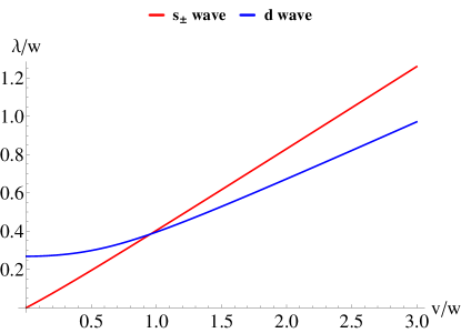
(a)

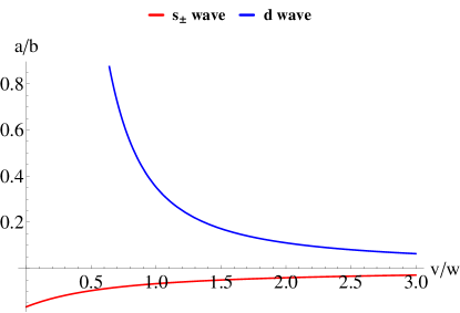
(b)

Figure S2: (a) Eigenvalue $\lambda$ of different superconducting states as a function of the ratio $v/w$ between intra-orbital pairing involving $d_{xz/yz}$ orbitals and $d_{xy}$ orbitals, respectively. (b) Ratio of the coefficients $a_{x}$ and $b_{x}$ of the gap in the electron pocket $e_{x}$, given in Eq. (S9), as function of $v/w$.

In the presence of orbital order, both $\beta_{e}$ and $\beta_{h}$ become non-zero. To reflect the fact that the RPA-derived pairing interaction between the hole pocket and the $e_{x}$ pocket is strongly enhanced by orbital order, we must set $\beta_{e}>\beta_{h}$. For concreteness, here we consider $\beta_{e}=2\beta_{h}$. Solving the linearized gap equations as function of $\beta_{e}$ we find an increase in the leading eigenvalue $\lambda$ when $w$ and $v$ are comparable, $v=1.2w$, (i.e. nearly-degenerate $s^{+-}$ and $d$-wave states), as shown in Fig. S3. Since $T_{c}\propto\mathrm{e}^{-1/\lambda}$, $T_{c}$ is enhanced by orbital order, in agreement with the RPA calculations.

As for the gap structure, we find that nodes are introduced in the hole pocket along the $x$ direction for $\beta_{e}\gtrsim 0.36$, when $c_{2}/c_{0}<-1$. In both electron pockets, nodes are expelled along the $x$ axis – in particular, they are expelled from $e_{x}$ for $\beta_{e}\gtrsim 0.16$ (when $a_{x}/b_{x}>0$) and from the $e_{y}$ pocket for $\beta_{e}\gtrsim 0.45$ (when $a_{y}/b_{y}<-1$). The fact that the nodes are expelled from the $e_{x}$ pocket before they leave the $e_{y}$ pocket also agrees with the RPA calculations.

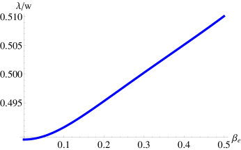
(a)

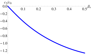
(b)

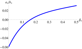
(c)

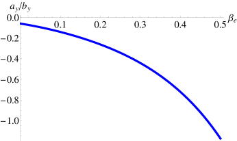
(d)

Figure S3: In the plots above, we set $\beta_{h}=\beta_{e}/2$ and $v/w=1.2$, placing the system near the degeneracy between $s^{+-}$ and $d$-wave. (a) Leading superconducting eigenvalue as a function of $\beta_{e}$. (b) Ratio of the leading coefficients $c_{0}$ and $c_{2}$ of the gap in the hole pocket $h_{1}$, given in Eq. (S9), as function of $\beta_{e}$. (c) Ratio of the coefficients $a_{x}$ and $b_{x}$ of the gap in the electron pocket $e_{x}$, given in Eq. (S9), as function of $\beta_{e}$. (d) Ratio of the coefficients $a_{y}$ and $b_{y}$ of the gap in the electron pocket $e_{y}$, given in Eq. (S9), as function of $\beta_{e}$.

Having established a model that captures the main features of the RPA calculation at $T_{c}$, we calculated the gap structure also for $T=0$ to check whether the nodal structure is robust with changes in temperature. We find that, independent of the value of the cutoff $\Lambda$, the gap structure at $T=0$ is very similar to the one at $T_{c}$, as shown in Fig. 3 of the manuscript.

II Anisotropic penetration depth

II.1 Scaling behavior of quadratic nodes

The penetration depth measured along the $\mu$ direction for a field applied in the $\mu$ direction is given by:

$$\Delta\lambda_{\mu\mu}\equiv\lambda_{\mu\mu}-\lambda_{0}=\alpha\int\mathrm{d}\omega\ \tilde{N}_{\mu\mu}(\omega)\left(-\frac{\partial f(\omega)}{\partial\omega}\right)$$ (S10)

where $\lambda_{0}$ is the $T=0$ value of the penetration depth, $\alpha$ is an overall pre-factor, $f\left(\omega\right)$ is the Fermi-Dirac distribution function, and $\tilde{N}\left(\omega\right)$ is the Fermi-velocity weighted density of states:

$$\tilde{N}_{\mu\mu}(\omega)=\sum_{j}\int d^{2}k\ \delta\left(\omega-E_{j}(\mathbf{k})\right)\left(v_{j,\mu}^{F}\right)^{2}$$ (S11)

Here, $E_{j}\left(\mathbf{k}\right)=\sqrt{\Delta_{j}^{2}\left(\mathbf{k}\right)+\varepsilon^{2}\left(\mathbf{k}\right)}$ is the quasi-particle dispersion of pocket $j$, with $\varepsilon\left(\mathbf{k}\right)=\frac{k^{2}}{2m}-\varepsilon_{F}$ assumed to be a parabolic dispersion. Note that, to focus on the effect caused by the changes in the gap function due to orbital order, we assume the four pockets to be the same – this simplification does not affect the main results below.

Let us consider the effect of a quadratic node on a single pocket. The quadratic node appears when the node is on the verge of being introduced in or expelled from the pocket. For concreteness, we consider the gap function on the electron pocket $j$:

$$\Delta_{j}\left(\phi_{j}\right)=\Delta_{0,j}\left(1-r\cos 2\phi_{j}\right)$$ (S12)

For the hole pockets, one only needs to change $\cos 2\phi_{j}$ to $\cos 4\phi_{j}$, and the results are similar. To avoid cumbersome expressions, we drop the subscript $j$ hereafter. Note that for $\left|r\right|>1$, accidental nodes are present, whereas for $\left|r\right|<1$, nodes are absent. Thus $r=\pm 1$ corresponds to the point where nodes disappear from (or appear in) the pocket. For $r=1$, the nodes are expelled along the $x$ direction ($\phi_{0}=0,\pi$), whereas for $r=-1$, they are expelled along the $y$ direction ($\phi_{0}=\pm\pi/2$). Expansion around either of these points gives $\Delta\left(\phi\right)\propto\left(\phi-\phi_{0}\right)^{2}$, hence the name quadratic nodes.

To illustrate the low-temperature scaling behavior of the anisotropic penetration depth, we consider the case $r=1$. Substituting in Eq. (S11) we obtain:

$$\tilde{N}_{xx}(\omega)= N_{0}v_{F}^{2}\omega\int\frac{d\phi}{2\pi}\ \frac{\cos^{2}\phi}{\sqrt{\omega^{2}-\Delta_{0}^{2}\left(1-\cos 2\phi\right)^{2}}}\theta\left(\omega-\Delta_{0}\left(1-\cos 2\phi\right)\right)$$

$$\tilde{N}_{yy}(\omega)= N_{0}v_{F}^{2}\omega\int\frac{d\phi}{2\pi}\ \frac{\sin^{2}\phi}{\sqrt{\omega^{2}-\Delta_{0}^{2}\left(1-\cos 2\phi\right)^{2}}}\theta\left(\omega-\Delta_{0}\left(1-\cos 2\phi\right)\right)$$ (S13)

where $\theta\left(x\right)$ is the step function. For $\omega\ll\Delta_{0}$, we can expand around the quadratic node $\phi_{0}=0$ to obtain:

$$\tilde{N}_{xx}(\omega)= N_{0}v_{F}^{2}\sqrt{\frac{\omega}{2\Delta_{0}}}\int_{-1}^{1}\frac{dz}{2\pi}\ \frac{1}{\sqrt{1-z^{4}}}\sim\sqrt{\omega}$$

$$\tilde{N}_{yy}(\omega)= N_{0}v_{F}^{2}\left(\frac{\omega}{2\Delta_{0}}\right)^{3/2}\int_{-1}^{1}\frac{dz}{2\pi}\ \frac{z^{2}}{\sqrt{1-z^{4}}}\sim\omega^{3/2}$$ (S14)

Substitution in Eq. (S10) then gives the low-temperature behavior $\Delta\lambda_{xx}\sim\sqrt{T}$ and $\Delta\lambda_{yy}\sim T^{3/2}$. Note that, if accidental linear nodes are present in other pockets, they will give a linear-in-$T$ contribution $\Delta\lambda_{\mu\mu}\sim T$ for both directions. Thus, while the quadratic nodes dominate the low-temperature behavior of the penetration depth along the $x$ direction, accidental linear nodes dominate the behavior of the penetration depth along the $y$ direction. Note also that for $r=-1$, when nodes are expelled from the pocket along the $y$ direction, one obtains the opposite behavior $\Delta\lambda_{xx}\sim T^{3/2}$ and $\Delta\lambda_{yy}\sim\sqrt{T}$.

II.2 Four-band model

To calculate how the anisotropic penetration depth changes as orbital order increases, we start with the expression that relates the gap structure in the presence of orbital order to a mixture of the $s^{+-}$ and $d$-wave gap structures of the tetragonal phase:

$$\Delta_{i}=\Delta_{i,s}+\gamma\Delta_{i,d}$$ (S15)

where $i$ denotes one of the four Fermi pockets. As discussed in the main text, increasing orbital order implies increasing the mixing coupling $\gamma$. Since the nodal structure at $T_{c}$ is very similar to the nodal structure at $T=0$ (Fig. 3 of the main paper), we write the gaps as the product of an overall temperature-dependent (but pocket-independent) amplitude $\Delta_{0}$ and a temperature-independent structure factor $g_{i,s/d}$, i.e. $\Delta_{i,s/d}=\Delta_{0}\,g_{i,s/d}$. Thus, we can obtain $g_{i,s/d}$ directly from the linearized gap equations in the tetragonal phase.

To capture the effects of the nodes that emerge in the outer hole pocket $h_{2}$, we expand our effective three-band model by including the normalized wave-function:

$$|h_{2}\rangle=\sin\theta\left|d_{xz}\right\rangle-\cos\theta\left|d_{yz}\right\rangle\ .$$ (S16)

such that $\left\langle\left.h_{2}\right|h_{1}\right\rangle=0$. Note that, in accord to the tight-binding model, the angular variation of the orbital content of $h_{2}$ is $\pi/2$ out of phase with respect to the angular variation of the orbital content of $h_{1}$. Since we will solve the linearized gap equations in the tetragonal phase, i.e. $\beta_{h}=\beta_{e}=0$, the pairing interactions in the band basis acquire the simplified form:

$$\Gamma_{xy} =\frac{\alpha^{4}W}{(\alpha^{2}+\sin^{2}\phi_{x})(\alpha^{2}+\cos^{2}\phi_{y})}$$ (S17)

$$\Gamma_{h_{1}x} =\frac{V\sin^{2}\phi_{x}\sin^{2}\theta}{\alpha^{2}+\sin^{2}\phi_{x}} \Gamma_{h_{1}y} =\frac{V\cos^{2}\phi_{y}\cos^{2}\theta}{\alpha^{2}+\cos^{2}\phi_{y}}$$ (S18)

$$\Gamma_{h_{2}x} =t\frac{V\sin^{2}\phi_{x}\cos^{2}\theta}{\alpha^{2}+\sin^{2}\phi_{x}} \Gamma_{h_{2}y} =t\frac{V\cos^{2}\phi_{y}\sin^{2}\theta}{\alpha^{2}+\cos^{2}\phi_{y}}\ .$$ (S19)

The RPA calculation reveals that the pairing interaction is greatly enhanced by the nesting between $h_{1}$ and the electron pockets KemperNJP . To account for the worse nesting conditions between $h_{2}$ and the electron pockets, we add a factor $t<1$ to the pairing interactions $\Gamma_{h_{2}x/y}$. For concreteness, here we set $t=2/3$.

The linearized gap equation can be conveniently expressed as an algebraic system of equations after writing the gap functions in terms of harmonic functions of the angle around the pockets, Eq. (S9). Note that, because we are in the tetragonal state, $c_{4}=c_{6}=0$ always. Solution of the gap equations reveals that the phase diagram is very similar to the three-band model, with the $s^{+-}$ and $d$-wave states becoming degenerate at $v/w\approx 0.8$.

To calculate the anisotropic penetration depth, we place the system near this degeneracy point – in particular, we set $v=w$. At $T=T_{c}$, the structure factors are then calculated in a straightforward way, yielding:

$$g_{s,h_{1}} =0.602\ , g_{s,h_{2}} =\dfrac{2}{3}g_{h_{1}}\ , g_{s,x} =\dfrac{0.061-0.897\sin^{2}\phi_{x}}{\alpha^{2}+\sin^{2}\phi_{x}}\ , g_{s,y} =\dfrac{0.061-0.897\cos^{2}\phi_{y}}{\alpha^{2}+\cos^{2}\phi_{y}}$$ (S20)

$$g_{d,h_{1}} =-0.640\cos 2\theta\ , g_{d,h_{2}} =-\dfrac{2}{3}g_{h_{1}}\ , g_{d,x} =-\dfrac{0.182+0.479\sin^{2}\phi_{x}}{\alpha^{2}+\sin^{2}\phi_{x}}\ , g_{d,y} =\dfrac{0.182+0.479\cos^{2}\phi_{y}}{\alpha^{2}+\cos^{2}\phi_{y}}$$

Substitution in Eq. (S15) and in the definition of the anisotropic penetration depth (S10) gives the result shown in Fig. 4 of the main text.

III Time-reversal symmetry breaking and orbital order

In this section we discuss under what conditions the mixing parameter $\gamma$ in Eq. (S15) is real or complex. Note that a comlex $\gamma$ effectively lifts the nodes that appear for a real $\gamma$. To analytically address this question, we simplify our three-band model further and ignore the angular dependence of the pairing interaction. Thus, the effect of orbital order is included only in the inter-pocket pairing interaction

$$\Gamma_{hx}=V(1+\varphi)\ ,\quad\Gamma_{hy}=V(1-\varphi)\ ,\mbox{ and}\quad\Gamma_{xy}=W\ ,$$ (S21)

where $\varphi$, the nematic order parameter, is proportional to the orbital order parameter (see also Ref. RMFSDMix ). For concreteness, we set $\Delta_{h}$ to be real and positive, and write $\Delta_{x}=\Delta_{1}\exp(i\theta_{1})$ and $\Delta_{y}=\Delta_{2}\exp(i\theta_{2})$, with $\Delta_{1,2}\geq 0$. In the absence of orbital order ($\varphi=0$), the $s^{+-}$ state takes place for $V>W$ and is characterized by $\theta_{1}=\theta_{2}=\pi$, whereas the $d$-wave state, taking place for $V<W$, has $\theta_{1}=0$, $\theta_{2}=\pi$. Thus, any solution in the presence of orbital order ($\varphi\neq 0$) with $\theta_{i}\neq 0,\pi$ necessarily implies that the mixing coefficient $\gamma$ in Eq. (S15) is complex. Note that $\theta_{i}\neq 0,\pi$ also implies that the superconducting state is time-reversal symmetry-breaking (TRSB), since $\Delta_{i}^{*}\neq\Delta_{i}$.

To proceed, we solve the $T=0$ BCS-like equations of this model. By denoting $v=VN_{0}$ and $w=WN_{0}$, where $N_{0}$ is the density of states at the Fermi energy, we have:

$$\left\{\begin{aligned} \Delta_{h}&=-v(1+\varphi)\Delta_{1}\ln\frac{2\Lambda}{\Delta_{1}}\cos\theta_{1}-v(1-\varphi)\Delta_{2}\ln\frac{2\Lambda}{\Delta_{2}}\cos\theta_{2}\\ 0&=-v(1+\varphi)\Delta_{1}\ln\frac{2\Lambda}{\Delta_{1}}\sin\theta_{1}-v(1-\varphi)\Delta_{2}\ln\frac{2\Lambda}{\Delta_{2}}\sin\theta_{2}\\ \Delta_{1}\cos\theta_{1}&=-v(1+\varphi)\Delta_{h}\ln\frac{2\Lambda}{\Delta_{h}}-w\Delta_{2}\ln\frac{2\Lambda}{\Delta_{2}}\cos\theta_{2}\\ \Delta_{1}\sin\theta_{1}&=-w\Delta_{2}\ln\frac{2\Lambda}{\Delta_{2}}\sin\theta_{2}\\ \Delta_{2}\cos\theta_{2}&=-v(1-\varphi)\Delta_{h}\ln\frac{2\Lambda}{\Delta_{h}}-w\Delta_{1}\ln\frac{2\Lambda}{\Delta_{1}}\cos\theta_{1}\\ \Delta_{2}\sin\theta_{2}&=-w\Delta_{1}\ln\frac{2\Lambda}{\Delta_{1}}\sin\theta_{1}\ .\end{aligned}\right.$$ (S22)

Solving Eq. S22, we find that the TRSB solution exists only when the following condition is satisfied

$$\left|\left(1+\varphi\right)-\frac{w}{v}\exp\left(\frac{1+\varphi}{w(1-\varphi)}-\frac{w}{v^{2}(1-\varphi^{2})}\right)\right|<(1-\varphi)\exp\left(\frac{4\varphi}{w(1-\varphi^{2})}\right)<$$

$$< \ \left(1+\varphi\right)+\frac{w}{v}\exp\left(\frac{1+\varphi}{w(1-\varphi)}-\frac{w}{v^{2}(1-\varphi^{2})}\right)$$ (S23)

In the tetragonal phase ($\varphi=0$), and in the weak-coupling limit $w,v\ll 1$, this condition reduces to

$$v-w<\frac{\ln 2}{2}w^{2}\ ,$$ (S24)

in agreement with Valentin ; Maiti . It is instructive to compare the TRS and TRSB solutions in this regime:

$$\mbox{TRS: }\left\{\begin{aligned} \Delta_{h}&=0\\ \Delta_{x}&=2\Lambda\exp(-1/w)\\ \Delta_{y}&=-2\Lambda\exp(-1/w)\end{aligned}\right.\qquad\mbox{TRSB: }\left\{\begin{aligned} \Delta_{h}&=2\Lambda\exp(-w/v^{2})\\ \left|\Delta_{x}\right|&=\left|\Delta_{y}\right|=2\Lambda\exp(-1/w)\\ \theta_{x}&=-\theta_{y}=\arccos\left(-\frac{w}{2v}\exp\left(\frac{1}{w}-\frac{w}{v^{2}}\right)\right)\end{aligned}\right.\ .$$ (S25)

From Eq. S25, it is clear that the TRSB state has a larger condensation energy $\sum_{i}\left|\Delta_{i}\right|^{2}$ than the TRS state, and is therefore the global energy minimum. Note however that in the regime $\frac{w}{v}-1\gg v$, $|\Delta_{h}|\ll|\Delta_{x/y}|$ and $\theta_{x}-\theta_{y}\approx\pi$. Therefore, as the system moves farther from the $s^{+-}$/$d$-wave degeneracy point $w=v$, the energy of the TRSB state asymptoticaly approaches the energy of the TRS state.

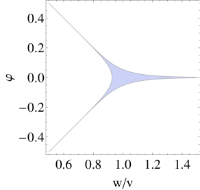
Figure S4: The shaded blue region, given by condition (S23), corresponds to the regime in which the superconducting ground state breaks time-reversal symmetry. Here, $\varphi$ is proportional to the orbital order parameter, and $w/v$ is the ratio between electron pocket-electron pocket and hole pocket-electron pocket pairing interactions. In this plot, $v=0.2$.

For non-zero orbital order, $\varphi\neq 0$, we solve Eq. (S23) numerically to find the region in the $\left(\frac{w}{v},\varphi\right)$ phase diagram for which the superconducting state is TRSB. As shown in Fig. S4, we find that orbital order in general suppresses the TRSB phase, which is restricted to the vicinity of the degeneracy point $w=v$. Note that, along the three very thin long branches in the plot, the condensation energy of the TRSB solution is lower but very close to the energy of the TRS solution (with $\theta_{1,2}=0,\pi$). The very long extension of these branches is an artifact of our simplified model, which can be eliminated if one includes angular-dependent terms in the pairing interaction (S21).

References

(1) Y. Kamihara, T. Watanabe, M. Hirano, and H. Hosono,
J. Am. Chem. Soc. 130, 3296 (2008).
(2) M. Rotter, M. Tegel, D. Johrendt, Phys. Rev. Lett.
101, 107006 (2008).
(3) H. Ding, P. Richard, K. Nakayama, K. Sugawara,
T. Arakane, Y. Sekiba, A. Takayama, S. Souma, T. Sato, T. Takahashi,
Z. Wang, X. Dai, Z. Fang, G. F. Chen, J. L. Luo, and N. L. Wang, Europhys.
Lett. 83, 47001 (2008).
(4) T. Shimojima, F. Sakaguchi, K. Ishizaka,
Y. Ishida, T. Kiss, M. Okawa, T. Togashi, C.T. Chen, S. Watanabe,
M. Arita, K. Shimada, H. Namatame, M. Taniguchi, K. Ohgushi, S. Kasahara,
T. Terashima, T. Shibauchi, Y. Matsuda, A. Chainani, and S. Shin,
Science 332, 564 (2011).
(5) M. A. Tanatar, J.-Ph. Reid, H. Shakeripour,
X. G. Luo, N. Doiron-Leyraud, N. Ni, S. L. Bud’ko, P. C. Canfield,
R. Prozorov, and L. Taillefer, Phys. Rev. Lett. 104, 067002
(2010).
(6) S.V. Borisenko, V. B. Zabolotnyy, A.A.
Kordyuk, D.V. Evtushinsky, T.K. Kim, I.V. Morozov, R. Follath, and
B. Büchner, Symmetry 4, 251 (2012).
(7) M. P. Allan, A. W. Rost, A. P. Mackenzie, Yang
Xie, J. C. Davis, K. Kihou, C. H. Lee, A. Iyo, H. Eisaki, T.-M. Chuang,
Science 336, 563 (2012).
(8) K. Hashimoto, M. Yamashita, S. Kasahara,
Y. Senshu, N. Nakata, S. Tonegawa, K. Ikada, A. Serafin, A. Carrington,
T. Terashima, H. Ikeda, T. Shibauchi, and Y. Matsuda, Phys. Rev. B
81, 220501(R) (2010).
(9) Y. Zhang, Z. R. Ye, Q. Q. Ge, F. Chen, Juan Jiang,
M. Xu, B. P. Xie, and D. L. Feng, Nature Phys. 8, 371 (2012).
(10) T. Yoshida, S. Ideta, T. Shimojima, W. Malaeb,
K. Shinada, H. Suzuki, I. Nishi, A. Fujimori, K. Ishizaka, S. Shin,
Y. Nakashima, H. Anzai, M. Arita, A. Ino, H. Namatame, M. Taniguchi,
H. Kumigashira, K. Ono, S. Kasahara, T. Shibauchi, T. Terashima, Y.
Matsuda, M. Nakajima, S. Uchida, Y. Tomioka, T. Ito, K. Kihou, C.
H. Lee, A. Iyo, H. Eisaki, H. Ikeda, R. Arita, T. Saito, S. Onari,
and H. Kontani, arXiv:1301.4818.
(11) X. Qiu, S. Y. Zhou, H. Zhang, B. Y. Pan,
X. C. Hong, Y. F. Dai, Man Jin Eom, Jun Sung Kim, Z. R. Ye, Y. Zhang,
D. L. Feng, and S. Y. Li, Phys. Rev. X 2, 011010 (2012).
(12) C.-L. Song, Y.-L. Wang, Y.-P. Jiang, W. Li, T.
Zhang, Z. Li, K. He, L. Wang, J.-F. Jia, H.-H. Hung, C. Wu, X. Ma,
X. Chen, and Q.-K. Xue, Science 332, 1410 (2011).
(13) K. Hashimoto, A. Serafin, S. Tonegawa,
R. Katsumata, R. Okazaki, T. Saito, H. Fukazawa, Y. Kohori, K. Kihou,
C. H. Lee, A. Iyo, H. Eisaki, H. Ikeda, Y. Matsuda, A. Carrington,
and T. Shibauchi, Phys. Rev. B 82, 014526 (2010).
(14) K. Okazaki, Y. Ota, Y. Kotani, W. Malaeb,
Y. Ishida, T. Shimojima, T. Kiss, S. Watanabe, C.-T. Chen, K. Kihou,
C. H. Lee, A. Iyo, H. Eisaki, T. Saito, H. Fukazawa, Y. Kohori, K.
Hashimoto, T. Shibauchi, Y. Matsuda, H. Ikeda, H. Miyahara, R. Arita,
A. Chainani, and S. Shin, Science 337, 1314 (2012).
(15) F. F. Tafti, A. Juneau-Fecteau, M.-E.
Delage, S. Rene de Cotret, J.-Ph. Reid, A. F. Wang, X.-G. Luo, X.
H. Chen, N. Doiron-Leyraud, and L. Taillefer, Nature Physics 9,
349 (2013).
(16) V. Zinth and D. Johrendt, Europhys. Lett.
98, 57010 (2012).
(17) I. I. Mazin, D. J. Singh, M. D. Johannes, and
M. H. Du, Phys. Rev. Lett. 101, 057003 (2008); A. V. Chubukov,
D. V. Efremov and I Eremin, Phys. Rev. B 78, 134512 (2008);
K. Kuroki, S. Onari, R. Arita, H. Usui, Y. Tanaka, H. Kontani, and
H. Aoki, Phys. Rev. Lett. 101, 087004 (2008); V. Cvetković
and Z. Tešanović, Phys. Rev. B 80, 024512 (2009); J.
Zhang, R. Sknepnek, R. M. Fernandes, and J. Schmalian, Phys. Rev.
B 79, 220502(R) (2009).
(18) A. V. Chubukov, Annu. Rev. Cond. Mat. Phys.
3, 57 (2012); P. J. Hirschfeld, M. M. Korshunov, and I. I.
Mazin, Rep. Prog. Phys. 74, 124508 (2011).
(19) X.-P. Wang, P. Richard, Y.-B. Huang, H.
Miao, L. Cevey, N. Xu, Y.-J. Sun, T. Qian, Y.-M. Xu, M. Shi, J.-P.
Hu, X. Dai, and H. Ding, Phys. Rev. B 85, 214518 (2012).
(20) M. Yi, D. Lu, J.-H. Chu, J. G. Analytis, A.
P. Sorini, A. F. Kemper, B. Moritz, S.-K. Mo, R. G. Moore, M. Hashimoto,
W.-S. Lee, Z. Hussain, T. P. Devereaux, I. R. Fisher, and Z.-X. Shen,
PNAS, 108, 6878 (2011).
(21) K. Kuroki, H. Usui, S. Onari, R. Arita, and H.
Aoki, Phys. Rev. B 79, 224511 (2009).
(22) S. Graser, T. A. Maier, P. J. Hirschfeld, and
D. J. Scalapino, New J. Phys. 11, 025016 (2009).
(23) A. V. Chubukov, M. G. Vavilov, and A. B. Vorontsov,
Phys. Rev. B 80, 140515(R) (2009).
(24) W.-C. Lee, S.-C. Zhang, and C. Wu, Phys. Rev. Lett.
102, 217002 (2009).
(25) A. F. Kemper, T. A. Maier, S. Graser, H.-P. Cheng,
P. J. Hirschfeld, D. J. Scalapino, New J. Phys. 12, 073030
(2010).
(26) S. Graser, A. F. Kemper, T. A. Maier, H.-P. Cheng,
P. J. Hirschfeld, and D. J. Scalapino, Phys. Rev. B 81, 214503
(2010).
(27) H. Ikeda, R. Arita, and J. Kunes, Phys. Rev. B
81, 054502 (2010).
(28) F. Wang, H. Zhai, and D.-H. Lee, Phys. Rev. B 81,
184512 (2010).
(29) S. Maiti, M. M. Korshunov, T. A. Maier, P. J. Hirschfeld,
and A. V. Chubukov, Phys. Rev. B 84, 224505 (2011); ibid
Phys. Rev. Lett. 107, 147002 (2011).
(30) R. Thomale, C. Platt, W. Hanke, J. Hu, and B.
A. Bernevig, Phys. Rev. Lett. 107, 117001 (2011).
(31) R. M. Fernandes and A. J. Millis, Phys. Rev.
Lett. 110, 117004 (2013).
(32) Z. P. Yin, K. Haule, and G. Kotliar, arxiv:1311.1188.
(33) F. Kretzschmar, B. Muschler, T. Böhm, A. Baum,
R. Hackl, H.-H. Wen, V. Tsurkan, J. Deisenhofer, and A. Loidl, Phys.
Rev. Lett. 110, 187002 (2013).
(34) M. Khodas, A. V. Chubukov, and G. Blumberg,
arXiv:1405.6246.
(35) J.-H. Chu, H.-H. Kuo, J. G. Analytis,
and I. R. Fisher, Science 337, 710 (2012).
(36) H.-H. Kuo, M. C. Shapiro, S. C. Riggs, and I. R.
Fisher, Phys. Rev. B 88, 085113 (2013).
(37) R. M. Fernandes, L. H. VanBebber, S. Bhattacharya,
P. Chandra, V. Keppens, D. Mandrus, M. A. McGuire, B. C. Sales, A.
S. Sefat, and J. Schmalian, Phys. Rev. Lett. 105, 157003
(2010).
(38) M. Yoshizawa, D. Kimura, T. Chiba, A. Ismayil,
Y. Nakanishi, K. Kihou, C.-H. Lee, A. Iyo, H. Eisaki, M. Nakajima,
and S. Uchida, J. Phys. Soc. Jpn. 81, 024604 (2012).
(39) S. Kasahara, H. J. Shi, K. Hashimoto, S. Tonegawa,
Y. Mizukami, T. Shibauchi, K. Sugimoto, T. Fukuda, T. Terashima, A.
H. Nevidomskyy, and Y. Matsuda, Nature 486, 382 (2012).
(40) A. E. Böhmer, P. Burger, F. Hardy, T. Wolf,
P. Schweiss, R. Fromknecht, M. Reinecker, W. Schranz, and C. Meingast,
Phys. Rev. Lett. 112, 047001 (2014).
(41) Y. Gallais, R. M. Fernandes, I. Paul, L.
Chauviere, Y.-X. Yang, M.-A. Measson, M. Cazayous, A. Sacuto, D. Colson,
and A. Forget, Phys. Rev. Lett. 111, 267001 (2013).
(42) A. Patz et al., Nature Comm. 5,
3229 (2014).
(43) E. P. Rosenthal, E. F. Andrade, C.
J. Arguello, R. M. Fernandes, L. Y. Xing, X. C. Wang, C. Q. Jin, A.
J. Millis, and A. N. Pasupathy, Nature Phys. 10, 225 (2014).
(44) J.-H. Chu, J. G. Analytis, K. De Greve, P. L.
McMahon, Z. Islam, Y. Yamamoto, and I. R. Fisher, Science 329,
824 (2010).
(45) M. A. Tanatar, E. C. Blomberg, A. Kreyssig, M.
G. Kim, N. Ni, A. Thaler, S. L. Bud’ko, P. C. Canfield, A. I. Goldman,
I. I. Mazin, and R. Prozorov, Phys. Rev. B 81, 184508 (2010).
(46) A. Lucarelli, A. Dusza, A. Sanna, S. Massidda,
J.-H. Chu, I.R. Fisher, and L. Degiorgi, New J. Phys. 14,
023020 (2012).
(47) C. Dhital et al., Phys. Rev. Lett. 108,
087001 (2012).
(48) R. M. Fernandes, A. V. Chubukov, and J. Schmalian,
Nature Phys. 10, 97 (2014).
(49) R. M. Fernandes, and A. J. Millis, Phys. Rev.
Lett. 111, 127001 (2013); F. Yang, F. Wang, and D.-H. Lee,
Phys. Rev. B 88, 100504 (2013).
(50) M. Yi et al., New J. Phys. 14, 073019
(2012).
(51) Y. Zhang et al., Phys Rev B 85,
085121 (2012).
(52) C. C. Lee, W. G. Yin, and W. Ku, Phys. Rev. Lett.
103, 267001 (2009).
(53) C.-C. Chen, J. Maciejko, A. P. Sorini, B. Moritz,
R. R. P. Singh, and T. P. Devereaux, Phys. Rev. B 82, 100504
(2010).
(54) W.-C. Lee and P. W. Phillips, Phys. Rev. B 86,
245113 (2012).
(55) S. Onari H. and Kontani, Phys. Rev. Lett. 109,
137001 (2012).
(56) S. Liang, A. Moreo, and E. Dagotto, Phys. Rev.
Lett. 111, 047004 (2013).
(57) R. M. Fernandes, A. V. Chubukov, J. Knolle,
I. Eremin, and J. Schmalian, Phys. Rev. B 85, 024534 (2012).
(58) W. Lv and P. Phillips, Phys. Rev. B 84, 174512
(2011).
(59) V. Cvetkovic and O. Vafek, Phys. Rev. B 88,
134510 (2013)
(60) V. Stanev and Z. Tesanovic, Phys. Rev. B 81,
134522 (2010).
(61) S. Maiti and A. V. Chubukov, Phys. Rev. B 87,
144511 (2013).
(62) R. M. Fernandes and J. Schmalian, Phys.
Rev. B 84, 012505 (2011).
(63) V. Stanev, B. S. Alexandrov, P. Nikolic,
and Z. Tesanovic, Phys. Rev. B 84, 014505 (2011).
(64) B. Mazidian, J. Quintanilla, A. D. Hillier,
and J. F. Annett, Phys. Rev. B 88, 224504 (2013).
(65) K. Hashimoto, K. Cho, T. Shibauchi,
S. Kasahara, Y. Mizukami, R. Katsumata, Y. Tsuruhara, T. Terashima,
H. Ikeda, M. A. Tanatar, H. Kitano, N. Salovich, R. W. Giannetta,
P. Walmsley, A. Carrington, R. Prozorov, and Y. Matsuda, Science 336,
1554 (2012).
(66) S. Kasahara et al., Phys. Rev. B 81,
184519 (2010).