Magnetic and orbital instabilities in a lattice of SU(4) organometallic Kondo complexes

Abstract

Motivated by experiments of scanning tunneling spectroscopy (STS) on self-assembled networks of iron(II)-phtalocyanine (FePc) molecules deposited on a clean Au(111) surface [FePc/Au(111)] and its explanation in terms of the extension of the impurity SU(4) Anderson model to the lattice in the Kondo regime, we study the competition between the Kondo effect and the magneto-orbital interactions occurring in FePc/Au(111). We explore the quantum phases and critical points of the model using a large-$N$ slave-boson method in the mean-field approximation. The SU(4) symmetry in the impurity appears as a combination of the usual spin and an orbital pseudospin arising from the degenerate $3d_{xz}$ and $3d_{yz}$ orbitals in the Fe atom. In the case of the lattice, our results show that the additional orbital degrees of freedom crucially modify the low-temperature phase diagram, and induce new types of orbital interactions among the Fe atoms, which can potentially stabilize exotic quantum phases with magnetic and orbital order. The dominant instability corresponds to spin ferromagnetic and orbital antiferromagnetic order.

1 Introduction

Organometallic complexes containing magnetic centers are currently under intense investigation for their potential uses as building blocks for nanotechnologies. Low-dimensional magnetic nanostructures have a high potential for applications in spintronics, magnetic recording and sensing devices [1, 2] These systems also offer a unique platform to study exotic phases of matter. In particular, Minamitani et al. [3] have shown that the Kondo effect observed in isolated iron(II) phtalocyanine (FePc) molecules deposited on top of clean Au(111) [FePc/Au(111)] (in the most usual on-top configuration) is a new realization of the SU(4) Kondo model, in which not only the spin degeneracy but also the orbital degeneracy between $3d_{xz}$ and $3d_{yz}$ orbitals of Fe play a role ($z$ is the direction normal to the surface). The SU(4) Kondo effect manifests itself as a dip at the Fermi energy in the differential conductance observed in scanning tunneling spectroscopy (STS). The half width at half maximum of the dip is about $T_{K}\sim$ 0.4 meV, with $T_{K}$ the Kondo temperature.

In another set of experiments, a self-organized square lattice of FePc/Au(111) as well as small clusters were studied by STS [4]. It was found that as for the isolated molecule, a single dip in the differential conductance remains for the molecules that lie at the corners of the clusters. However, increasing the coordination, the peak tends to split and for the lattice, a clear splitting of approximately 2 meV becomes apparent. Romero and the present authors were able to explain these experimental results, using a natural generalization of the single-impurity SU(4) Anderson model to the lattice, including hoppings between effective orbitals of nearest-neighbor molecules respecting the symmetry of these orbitals [5]. The relevant effective orbitals (i.e., the closest to the Fermi level), are essentially the $3d_{xz}$ and $3d_{yz}$ of Fe, with some admixture of other orbitals of the molecule. The splitting of the Kondo dip is a consequence of the anisotropy in the hopping for a given effective orbital.

Preliminary results suggests that the square lattice of FePc/Au(111)FePc is not far from a magnetic instability [5]. Ferromagnetic order was observed in a two-dimensional layer of organic molecules absorbed on graphene [6] and in metal-organic networks on Au surfaces [7, 8]. In addition, magnetic and orbital ordering are intertwined [9, 10].

In this work, starting from the orbitally degenerate Hubbard-Anderson model that describes the observed STS in different arrays of FePc molecules [5], we perform a Schrieffer-Wolff transformation to obtain an effective model which includes spin and orbital interactions. Solving this model in a slave-boson mean-field approximation (SBMFA), we obtain the critical values of the interactions leading to different symmetry-breaking magnetic and orbital instabilities. The dominant one turns out to be a spin ferromagnetic and orbital antiferromagnetic order. We show that the effect of the Ruderman-Kittel-Kasuya-Yosida (RKKY) interactions is small and can be neglected.

2 The Hubbard-Anderson model

Our starting model was derived Ref. [5] and discussed in detail in the supplemental material of that paper. The Hamiltonian $H=H_{1}+H_{2}$ can be separated into one-body ($H_{1}$) and two-body ($H_{2}$) parts. The first one can be written as

$$H_{1} = \sum_{ij}^{N}[E_{h}n_{\mathbf{r}_{ij}}-\sum_{\sigma\nu}\left(t_{2}h_{\mathbf{r}_{ij},\sigma}^{\nu\dagger}h_{\mathbf{r}_{ij}\pm\mathbf{a}_{\nu},\sigma}^{\nu}+t_{1}h_{\mathbf{r}_{ij},\sigma}^{\bar{\nu}\dagger}h_{\mathbf{r}_{ij}\pm\mathbf{a}_{\nu},\sigma}^{\bar{\nu}}\right)+\sum_{\xi\sigma\nu}\epsilon_{\xi}c_{\mathbf{r}_{ij},\xi,\sigma}^{\nu\dagger}c_{\mathbf{r}_{ij},\xi,\sigma}^{\nu}$$ (1)

$$+ V\sum_{\xi\sigma\nu}\left(h_{\mathbf{r}_{ij},\sigma}^{\nu\dagger}c_{\mathbf{r}_{ij},\xi,\sigma}^{\nu}+\rm{H.c.}\right)].$$

Here the operators $h_{\mathbf{r}_{ij},\sigma}^{\nu}$ annihilate a hole (create an electron) in the state $|\nu_{\mathbf{r}_{ij},\sigma}\rangle$, where $\nu=\left(x,y\right)$ denotes one of the two orbitally degenerate molecular states with spin $\sigma$ at site with position $\mathbf{r}_{ij}$ of the square lattice. $n_{\mathbf{r}_{ij}}=\sum_{\sigma\nu}n_{\mathbf{r}_{ij},\sigma}^{\nu}$, with $n_{\mathbf{r}_{ij},\sigma}^{\nu}=h_{\mathbf{r}_{ij},\sigma}^{\nu\dagger}h_{\mathbf{r}_{ij},\sigma}^{\nu}$ is the total number of holes at the molecule lying at site $ij$. The lattice vectors $\mathbf{a}_{\nu}$ connect nearest-neighbor sites, $\bar{x}=y$, and$\ \bar{y}=x$. The operator $c_{\mathbf{r}_{ij},\xi,\sigma}$ annihilates a conduction hole with spin $\sigma$ and quantum number $\xi$ at position $\mathbf{r}_{ij}$. The first and second terms of  $H_{1}$ describe the molecular states and the hopping between them. The hopping $t_{2}$ between $x$ ($y$) orbitals in the $x$ ($y$) direction is larger than the hopping $t_{1}$ between $x$ ($y$) orbitals in the $y$ ($x$) direction. The third term of  $H_{1}$ corresponds to a band of bulk and surface conduction electrons of the substrate and the last term is the hybridization between molecular and conduction states.

The interaction term can be written as [10, 11]

$$H_{2} = \sum_{ij}^{N}\left[U\sum_{\nu}n_{\mathbf{r}_{ij},\uparrow}^{\nu}n_{\mathbf{r}_{ij},\downarrow}^{\nu}+\sum_{\sigma\sigma^{\prime}}[(U-2J_{H})n_{\mathbf{r}_{ij},\sigma}^{x}n_{\mathbf{r}_{ij},\sigma^{\prime}}^{y}+J_{H}h_{\mathbf{r}_{ij},\sigma}^{x\dagger}h_{\mathbf{r}_{ij},\sigma^{\prime}}^{y\dagger}h_{\mathbf{r}_{ij},\sigma^{\prime}}^{x}h_{\mathbf{r}_{ij},\sigma}^{y}]\right.$$ (2)

$$+ \left.J_{H}\sum_{\nu}h_{\mathbf{r}_{ij},\uparrow}^{\nu\dagger}h_{\mathbf{r}_{ij},\downarrow}^{\nu\dagger}h_{\mathbf{r}_{ij},\downarrow}^{\bar{\nu}}h_{\mathbf{r}_{ij},\uparrow}^{\bar{\nu}}\right].$$

For the system we are considering, the occupation of the molecular states is nearly one-hole per site ($\left\langle n_{\mathbf{r}_{ij}}\right\rangle\sim 1$) and the main effect of $H_{2}$ is to inhibit double occupancy. Therefore as a first approximation one can take $U\longrightarrow+\infty$ and therefore neglect the Hund rules exchange $J_{H}$ in comparison with $U$. In this case, the interaction takes the simpler form $H_{2}^{s}=\frac{U}{2}\sum_{ij}^{N}n_{\mathbf{r}_{ij}}\left(n_{\mathbf{r}_{ij}}-1\right)$.

3 Symmetry of $H_{i}$

For the case of one molecule only, the resulting impurity Anderson Hamiltonian has SU(4) symmetry, which in simple terms means that permutations of the four states $\left|\nu_{\sigma}\right\rangle$ leave the Hamiltonian invariant. The fifteen generators of the SU(4) symmetry are three trivial diagonal matrices, six permutations of two states and other six permutations with a change of phases for the permuted states [12]. The twelve non trivial generators can also be written as a generalization of the raising and lowering operators for SU(2) [13]. Specifically, for the impurity Anderson model they are $S_{\nu\sigma}^{\nu^{\prime}\sigma^{\prime}}=\left(h_{\sigma}^{\nu\dagger}h_{\sigma^{\prime}}^{\nu^{\prime}}+\sum_{\xi}c_{\xi,\sigma}^{\nu\dagger}c_{\xi,\sigma^{\prime}}^{\nu^{\prime}}\right)$ for $\nu\sigma\neq\nu^{\prime}\sigma^{\prime}$ (note that the conduction electron degrees of freedom must be taken into account to keep the SU(4) symmetry of the total system.)

For the lattice, the simplest generalization of these generators leads to $S_{\nu\sigma}^{\nu^{\prime}\sigma^{\prime}}=\sum_{ij}^{N}\left(h_{\mathbf{r}_{ij},\sigma}^{\nu\dagger}h_{\mathbf{r}_{ij},\sigma^{\prime}}^{\nu^{\prime}}+\sum_{\xi}c_{\mathbf{r}_{ij},\xi,\sigma}^{\nu\dagger}c_{\mathbf{r}_{ij},\xi,\sigma^{\prime}}^{\nu^{\prime}}\right)$. All these generators commute with $H_{2}^{s}$, but those with $\nu\neq\nu^{\prime}$ commute with $H_{1}$ only in the particular case $t_{2}=t_{1}$, which seems incompatible with the observed STS in the square lattice of FePc/Au(111) [5]. In the general case, $t_{2}\neq t_{1}$, $H_{1}$ has however SU(4) symmetry with the following non-trivial generators $S_{\nu\sigma}^{\nu\bar{\sigma}}=\sum_{ij}^{N}\left(h_{\mathbf{r}_{ij},\sigma}^{\nu\dagger}h_{\mathbf{r}_{ij},\bar{\sigma}}^{\nu}+\sum_{\xi}c_{\mathbf{r}_{ij},\xi,\sigma}^{\nu\dagger}c_{\mathbf{r}_{ij},\xi,\bar{\sigma}}^{\nu}\right)$ and $S_{\nu\sigma}^{\bar{\nu}\sigma^{\prime}}=\sum_{ij}^{N}\left(h_{\mathbf{r}_{ij},\sigma}^{\nu\dagger}h_{R\mathbf{r}_{ij},\sigma^{\prime}}^{\bar{\nu}}+\sum_{\xi}c_{\mathbf{r}_{ij},\xi,\sigma}^{\nu\dagger}c_{R\mathbf{r}_{ij},\xi,\sigma^{\prime}}^{\bar{\nu}}\right)$, where $R$ is the reflection that permutes $x$ and $y$ (it is an element of the point group $C_{4v}$ of the system). It can be verified easily that these generators commute with $H_{1}$. However, inclusion of $H_{2}$ reduces the symmetry to spin SU(2) times orbital Z${}_{2}\times$U(1). Only the term of $H_{2}^{s}$ with $\mathbf{r}_{ij}=0$ commutes with the $S_{\nu\sigma}^{\bar{\nu}\sigma^{\prime}}$ generators which contain $R$. Nevertheless, in a Fermi liquid, the interaction becomes irrelevant at the Fermi energy and we expect that SU(4) is an emergent symmetry at low energies [14] if there is not a symmetry breaking (a magnetic or orbital instability). In fact, in the SBMFA, where the action is reduced to an effective non-interacting one near the Fermi energy [5] or in a dynamical-mean field approximation in which the interaction is treated exactly at one site in an effective medium, the effective model has SU(4) symmetry if the symmetric form $H_{2}^{s}$ is taken.

4 Effective generalized Heisenberg interactions

When two nearest-neighbor sites are singly occupied and if $U\gg t_{i}$ (as it seems to be the case for FePc/Au(111) [5], the hopping terms connecting these sites can be eliminated by means of a canonical transformation, in a similar fashion as the $t-J$ model is derived from the Hubbard model. This leads to an effective exchange model for spins and orbitals, as in the Kugel-Khomskii model [9, 10]. For simplicity we write first the result using the SU(4) symmetric form of the interaction $H_{2}^{s}$. After a lengthy but straightforward algebra we obtain

$$H_{H} =\sum_{i}\sum_{\nu}\left[\frac{4t_{2}^{2}}{U}\mathbf{S}_{i}^{\nu}\cdot\mathbf{S}_{i+\nu}^{\nu}+\frac{4t_{1}^{2}}{U}\mathbf{S}_{i}^{\bar{\nu}}.\mathbf{S}_{i+\nu}^{\bar{\nu}}\right]+\sum_{i}\sum_{\nu}\left[\frac{t_{2}^{2}+t_{1}^{2}}{4U}\left(4T_{i}^{z}T_{i+\nu}^{z}-3\right)\right]$$ (3)

$$+\sum_{i}\sum_{\nu}\frac{2t_{1}t_{2}}{U}\left(T_{i}^{-}T_{i+\nu}^{+}+T_{i}^{+}T_{i+\nu}^{-}\right)\left(\frac{1}{2}+2\mathbf{S}_{i}\cdot\mathbf{S}_{i+\nu}\right),$$

where $\mathbf{S}_{i}^{\nu}=\sum_{\alpha\beta}h_{i\alpha}^{\nu\dagger}{\mathbf{\sigma}}_{\alpha\beta}h_{i\beta}^{\nu}/2$ is the spin of the orbital $\nu$ at site $i$, and $\mathbf{S}_{i}=\sum_{\nu}\mathbf{S}_{i}^{\nu}$. The operator $\mathbf{T}_{i}$ denotes the orbital SU(2) pseudospin (with the identification of $x$ for pseudospin up). The subscript $i+\nu$ denotes the nearest neighbor of $i$ in the $+\nu$ direction. Note that in the case $t_{1}=t_{2}=t$, this Hamiltonian reduces to

$$H_{H}^{SU(4)}=\frac{2t^{2}}{U}\sum_{i}\sum_{\nu}\left(2\mathbf{S}_{i}\cdot\mathbf{S}_{i+\nu}+\frac{1}{2}\right)\left(2\mathbf{T}_{i}\cdot\mathbf{T}_{i+\nu}+\frac{1}{2}\right)+\rm{cte}.$$ (4)

where we have used that $\mathbf{S}_{i}^{\nu}\cdot\mathbf{S}_{i+\nu}^{\nu}+\mathbf{S}_{i}^{\bar{\nu}}\cdot\mathbf{S}_{i+\nu}^{\bar{\nu}}=\mathbf{S}_{i}\cdot\mathbf{S}_{i+\nu}\left(2T_{i}^{z}T_{i+\nu}^{z}+1/2\right)$. This Hamiltonian is a sum of products of a spin SU(2) invariant form (first factor) times a pseudospin SU(2) invariant (last factor). Thus, it is explicitly SU(2)$\times$SU(2) invariant. However, it has been shown [13] that the symmetry of $H_{H}^{SU(4)}$ is actually SU(4), which is larger than SU(2)$\times$SU(2).

When $t_{1}$ and $t_{2}$ are very different, as in the realistic case for for FePc/Au(111) [5], the first two terms of $H_{H}$ Eq. (3) are the most important ones. The first one is optimized for orbital ferromagnetic and spin antiferromagnetic order, while the second one favors orbital antiferromagnetic order. In a classical picture, the energy of both orders would be the same, $-(t_{1}^{2}+t_{2}^{2})/U$ per site. However when Hund rules are included [the form $H_{2}$, Eq. (2) is used for the interaction] the spin ferromagnetic order is favored. Projecting over intermediate double occupied triplet states, the dominant term of $H_{H}$ takes the form

$$H_{H}^{d}=\frac{J}{2}\sum_{\mathbf{r}_{ij},\mathbf{a}}\left(-1+4T_{\mathbf{r}_{ij}}^{z}T_{\mathbf{r}_{ij}+\mathbf{a}}^{z}\right)\left(\frac{3}{4}+\mathbf{S}_{\mathbf{r}_{ij}}.\mathbf{S}_{\mathbf{r}_{ij}+\mathbf{a}}\right),\hskip 28.45274pt{\rm}J=\frac{t_{1}^{2}+t_{2}^{2}}{2(U-3J_{H})}$$ (5)

5 Instabilities due to $H_{H}$

The simplest SBMFA of $H$ [5] is not enough to treat the magnetic and orbital instabilities. As it is usually done in mean-field treatments of the Kondo lattice, in which the RKKY interaction should be included explicitly [15], in this section we consider $H+H_{H}^{d}$ within the SBMFA to study the instabilities induced by $H_{H}^{d}$. In this approximation, the limit $U\rightarrow+\infty$ is taken with a constraint of forbidden double occupancy. However, the effects of a finite $U$ are considered explicitly in $H_{H}$.

As before [5], the hole operators are written in terms of auxiliary particles as $h_{\mathbf{r}_{ij},\sigma}^{\nu}=b_{\mathbf{r}_{ij}}^{\dagger}f_{\mathbf{r}_{ij},\sigma}^{\nu}$. The spin and pseudospin operators take the form

$$\mathbf{S}_{\mathbf{r}_{ij}}\equiv-\frac{1}{2}\sum_{\sigma,\nu}f_{\mathbf{r}_{ij},\sigma}^{\nu\dagger}\hat{\mathbf{\sigma}}_{\sigma,\sigma^{\prime}}f_{\mathbf{r}_{ij},\sigma^{\prime}}^{\nu},\hskip 14.22636pt\mathbf{T}_{\mathbf{r}_{ij}}\equiv-\frac{1}{2}\sum_{\sigma,\nu}f_{\mathbf{r}_{ij},\sigma}^{\nu\dagger}\hat{\tau}_{\nu,\nu^{\prime}}f_{\mathbf{r}_{ij},\sigma}^{\nu^{\prime}},$$ (6)

We also define the mixed operator $U_{\mathbf{r}_{ij}}^{z}\equiv S_{\mathbf{r}_{ij}}^{z}T_{\mathbf{r}_{ij}}^{z}=\frac{1}{4}\sum_{\sigma,\nu}\eta\left(\sigma\right)\eta\left(\nu\right)f_{\mathbf{r}_{ij},\sigma}^{\nu\dagger}f_{\mathbf{r}_{ij},\sigma}^{\nu}$, where $\eta\left(\uparrow\right)=\eta\left(x\right)=+1$ and $\eta\left(\downarrow\right)=\eta\left(y\right)=-1$, and where the constraint of no double occupation has been used.

Without loss of generality, we can assume that the ferromagnetic spin order occurs along the $\hat{z}$ axis. Then $H_{H}^{d}$ can be written as

$$H_{H}^{d}=\frac{J}{2}\sum_{\mathbf{r}_{ij},\mathbf{a}}\left[-S_{\mathbf{r}_{ij}}^{z}S_{\mathbf{r}_{ij}+\mathbf{a}}^{z}+3T_{\mathbf{r}_{ij}}^{z}T_{\mathbf{r}_{ij}+\mathbf{a}}^{z}+4U_{\mathbf{r}_{ij}}^{z}U_{\mathbf{r}_{ij}+\mathbf{a}}^{z}\right]+\rm{cst},$$ (7)

We now introduce the following Hubbard-Stratonovich (HS) decouplings

$$-\frac{J}{2}\sum_{\mathbf{r}_{ij},\mathbf{a}}S_{\mathbf{r}_{ij}}^{z}.S_{\mathbf{r}_{ij}+\mathbf{a}}^{z} \rightarrow\sum_{\mathbf{r}_{ij},\mathbf{a}}\left[\frac{1}{2J}m_{\mathbf{r}_{ij}}m_{\mathbf{r}_{ij}+\mathbf{a}}+\frac{1}{2}m_{\mathbf{r}_{ij}+\mathbf{a}}S_{\mathbf{r}_{ij}}^{z}+\frac{1}{2}m_{\mathbf{r}_{ij}}S_{\mathbf{r}_{ij}+\mathbf{a}}^{z}\right],$$ (8)

$$\frac{3J}{2}\sum_{\mathbf{r}_{ij},\mathbf{a}}T_{\mathbf{r}_{ij}}^{z}T_{\mathbf{r}_{ij}+\mathbf{a}}^{z} \rightarrow\sum_{\mathbf{r}_{ij},\mathbf{a}}\left[-\frac{1}{6J}n_{\mathbf{r}_{ij}}n_{\mathbf{r}_{ij}+\mathbf{a}}+\frac{1}{2}n_{\mathbf{r}_{ij}+\mathbf{a}}T_{\mathbf{r}_{ij}}^{z}+\frac{1}{2}n_{\mathbf{r}_{ij}}T_{\mathbf{r}_{ij}+\mathbf{a}}^{z}\right],$$ (9)

$$2J\sum_{\mathbf{r}_{ij},\mathbf{a}}U_{\mathbf{r}_{ij}}^{z}U_{\mathbf{r}_{ij}+\mathbf{a}}^{z} \rightarrow\sum_{\mathbf{r}_{ij},\mathbf{a}}\left[-\frac{8}{J}p_{\mathbf{r}_{ij}}p_{\mathbf{r}_{ij}+\mathbf{a}}+4p_{\mathbf{r}_{ij}}U_{\mathbf{r}_{ij}+\mathbf{a}}^{z}+4p_{\mathbf{r}_{ij}+\mathbf{a}}U_{\mathbf{r}_{ij}}^{z}\right],$$ (10)

where $m_{\mathbf{r}_{ij}}$ is related to the usual magnetization order parameter, $n_{\mathbf{r}_{ij}}$ is the orbital order parameter and $p_{\mathbf{r}_{ij}}$ is a magneto-orbital order parameter. In order for Eqs. (9) and (10) to be well-defined HS decouplings, the fields $n_{\mathbf{r}_{ij}}$ and $p_{\mathbf{r}_{ij}}$ should have antiferromagnetic order. Introducing the Fourier decompositions

$$m_{\mathbf{r}_{ij}}=\sum_{\mathbf{q}}\frac{e^{i\left(\mathbf{Q}_{m}+\mathbf{q}\right)\mathbf{r}_{ij}}}{\sqrt{N}}m_{\mathbf{q}},\ \ n_{\mathbf{r}_{ij}}=\sum_{\mathbf{q}}\frac{e^{i\left(\mathbf{Q}_{n}+\mathbf{q}\right)\mathbf{r}_{ij}}}{\sqrt{N}}n_{\mathbf{q}},\ \ p_{\mathbf{r}_{ij}}=\sum_{\mathbf{q}}\frac{e^{i\left(\mathbf{Q}_{p}+\mathbf{q}\right)\mathbf{r}_{ij}}}{\sqrt{N}}p_{\mathbf{q}},$$ (11)

where $\mathbf{Q}_{m}=\left(0,0\right)$ and $\mathbf{Q}_{n}=\mathbf{Q}_{p}=\mathbf{Q}=\left(\frac{\pi}{a_{0}},\frac{\pi}{a_{0}}\right)$, $H_{H}^{d}$ becomes

$$H_{H}^{d} = \sum_{\mathbf{q},\mathbf{a}}e^{-i\mathbf{q}\mathbf{a}}\left[\frac{\beta}{2J}m_{\mathbf{q}}m_{-\mathbf{q}}-m_{\mathbf{q}}\sum_{\nu}\frac{1}{\sqrt{N}}\sum_{\mathbf{k},\omega_{n}}\frac{1}{2}\left(\bar{f}_{\mathbf{k},\uparrow}^{\nu}f_{\mathbf{k}-\mathbf{q},\uparrow}^{\nu}-\bar{f}_{\mathbf{k},\downarrow}^{\nu}f_{\mathbf{k}-\mathbf{q},\downarrow}^{\nu}\right)_{\omega_{n}}\right]$$ (12)

$$+ \sum_{\mathbf{q},\mathbf{a}}e^{-i\mathbf{q}\mathbf{a}}\left[\frac{\beta}{6J}n_{\mathbf{q}}n_{-\mathbf{q}}-n_{\mathbf{q}}\sum_{\sigma}\frac{1}{\sqrt{N}}\sum_{\mathbf{k},\omega_{n}}\frac{1}{2}\left(\bar{f}_{\mathbf{k},\sigma}^{x}f_{\mathbf{k}-\left(\mathbf{Q}+\mathbf{q}\right),\sigma}^{x}-\bar{f}_{\mathbf{k},\sigma}^{y}f_{\mathbf{k}-\left(\mathbf{Q}+\mathbf{q}\right),\sigma}^{y}\right)_{\omega_{n}}\right]$$

$$+ \sum_{\mathbf{q},\mathbf{a}}e^{-i\mathbf{q}\mathbf{a}}\left[\frac{\beta 8}{J}p_{\mathbf{q}}p_{-\mathbf{q}}-p_{\mathbf{q}}\sum_{\sigma\nu}\frac{1}{\sqrt{N}}\sum_{\mathbf{k},\omega_{n}}2\eta\left(\sigma\right)\eta\left(\nu\right)\left(\bar{f}_{\mathbf{k},\sigma}^{\nu}f_{\mathbf{k}-\left(\mathbf{Q}+\mathbf{q}\right),\sigma}^{\nu}\right)_{\omega_{n}}\right],$$

The minimum of the free energy with respect to the order parameters defines the saddle-point equations

$$m_{\mathbf{q}} = J\sum_{\nu}\frac{1}{\beta N}\sum_{\mathbf{k},\omega_{n}}\frac{1}{2}\left\langle\bar{f}_{\mathbf{k},\uparrow}^{\nu}\left(i\omega_{n}\right)f_{\mathbf{k}+\mathbf{q},\uparrow}^{\nu}\left(i\omega_{n}\right)-\bar{f}_{\mathbf{k},\downarrow}^{\nu}\left(i\omega_{n}\right)f_{\mathbf{k}+\mathbf{q},\downarrow}^{\nu}\left(i\omega_{n}\right)\right\rangle,$$ (13)

$$n_{\mathbf{q}} = 3J\sum_{\sigma}\frac{1}{\beta N}\sum_{\mathbf{k},\omega_{n}}\frac{1}{2}\left\langle\bar{f}_{\mathbf{k},\sigma}^{x}\left(i\omega_{n}\right)f_{\mathbf{k}-\left(\mathbf{Q}-\mathbf{q}\right),\sigma}^{x}\left(i\omega_{n}\right)-\bar{f}_{\mathbf{k},\sigma}^{y}\left(i\omega_{n}\right)f_{\mathbf{k}-\left(\mathbf{Q}-\mathbf{q}\right),\sigma}^{y}\left(i\omega_{n}\right)\right\rangle,$$ (14)

$$p_{\mathbf{q}} = \frac{J}{4}\sum_{\sigma\nu}\frac{1}{\beta N}\sum_{\mathbf{k},\omega_{n}}2\eta\left(\sigma\right)\eta\left(\nu\right)\left\langle\bar{f}_{\mathbf{k},\sigma}^{\nu}\left(i\omega_{n}\right)f_{\mathbf{k}-\left(\mathbf{Q}-\mathbf{q}\right),\sigma}^{\nu}\left(i\omega_{n}\right)\right\rangle.$$ (15)

In order to determine which of these order parameters is the first to develop, we compute the change of sign in the second derivative of the free energy in the symmetric phase. This leads to the following conditions for the critical value of $J$ for each instability (similar to Stoner criteria)

$$\frac{1}{J_{c,m}}=\chi\left(\mathbf{0},0\right),\ \ \frac{1}{J_{c,n}}=3\chi\left(\mathbf{Q},0\right),\ \ \frac{1}{J_{c,p}}=4\chi\left(\mathbf{Q},0\right),\rm{}$$ (16)

where we have defined the static susceptibility of the electronic system,

$$\chi\left(\mathbf{q},0\right)\equiv\chi\left(\mathbf{q},\omega=0\right)=-\frac{4}{\beta N}\sum_{\mathbf{k},\omega_{n}}\frac{G_{\nu,\sigma}^{ff}\left(\mathbf{k},i\omega_{n}\right)-G_{\nu,\sigma}^{ff}\left(\mathbf{k}+\mathbf{q},i\omega_{n}\right)}{\epsilon_{\mathbf{k}}-\epsilon_{\mathbf{k}+\mathbf{q}}},$$ (17)

and the pseudofermion Green function is given in [5]

The problem now reduces to computing Eq. (17) for a generic $\mathbf{q}$. Performing the Matsubara sum at $T=0$ we obtain

$$\chi\left(\mathbf{q},0\right)=\frac{4}{N}\sum_{\mathbf{k}}\frac{1}{\pi}\frac{\arctan\left(\frac{E_{h}+\lambda+\epsilon_{\mathbf{k}}}{z^{2}\Gamma}\right)-\arctan\left(\frac{E_{h}+\lambda+\epsilon_{\mathbf{k}+\mathbf{q}}}{z^{2}\Gamma}\right)}{\epsilon_{\mathbf{k}}-\epsilon_{\mathbf{k}+\mathbf{q}}},$$ (18)

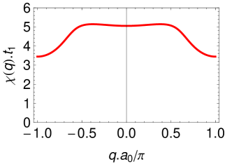
where $z=\left\langle b_{\mathbf{r}_{ij}}^{\dagger}\right\rangle$, $\lambda$ is a Lagrange multiplier used to impose the constraint $z^{2}+\sum_{\sigma,\nu=x,y}f_{\mathbf{r}_{ij},\sigma}^{\nu\dagger}f_{\mathbf{r}_{ij},\sigma}^{\nu}=1$, $W$ is half the band width and $\Gamma$ the resonant level width of the isolated impurity. This function is represented in Fig. 1

Figure 1: Susceptibility $\chi\left(\mathbf{q},0\right)$ vs $\mathbf{q}$ in the (1,1) direction.

For $\mathbf{q}\rightarrow 0$ we recover the usual expression $\chi\left(\mathbf{0},0\right)=\rho_{f}^{t}\left(0\right)$, where $\rho_{f}^{t}\left(0\right)$ is the total spectral density (summing over spin and orbital) at the Fermi level. For the parameters $\lambda,z$ that minimize the SBMFA action, we obtain $\chi\left(0,0\right)=5.05/t_{1}$, $\chi\left(\mathbf{Q},0\right)=3.45/t_{1}$ which replaced in Eq. (16) lead to the following critical values ($t_{1}=0.007$ eV)

$$J_{c,m}\approx 16.1{\rm K},\ \ J_{c,n}\approx 7.9{\rm K},\ \ J_{c,p}\approx 5.9\ {\rm K}.$$ (19)

We conclude that the first instability occurs in the magneto-orbital channel.

For FePc/Au(111) one can estimate $t_{1}=0.007$ eV, $t_{2}=3t_{1}$ and $U=1.6$ eV [5]. The exchange constant $J_{H}$ is difficult to estimate for effective molecular orbitals. For pure Fe orbitals it is of the order of 0.7 eV. From these estimates and the second Eq. (5), one expects $J\geq 1.8$ K. Thus, one might infer that the system is not too far from an instability against spin ferro- and orbital antiferro-magnetic order.

6 RKKY interactions

Another possible source of magnetic instabilities is the RKKY interaction, which consists in the indirect interaction $I$ between spins mediated by conduction electrons generated by the effective Kondo coupling between spins and conduction electrons $J_{K}\mathbf{S}_{i}\cdot\mathbf{s}_{i}$ at second order in $J_{K}$, where $\mathbf{s}_{i}$ is the spin of the conduction electrons at site $i.$

An advantage of Au and its (111) surface is that both the bulk sates and the surface Shockley states near the Fermi energy can be described as free electrons and therefore the calculations in Ref. [16] for three dimensions (3D) and Ref. [17] for the 2D case are valid. Following these works one can write for dimension N=2 or 3 for two spins $\mathbf{S}_{1}$ and $\mathbf{S}_{2}$ at a distance $R$ (we will consider nearest neighbors only)

$$H_{RKKY}\left(R\right)=I_{\rm{ND}}\left(R\right)\mathbf{S}_{1}.\mathbf{S}_{2},\ \ \ \ I_{\rm{ND}}\left(R\right)=-\frac{1}{4}\tilde{J}_{\rm{ND}}^{2}\chi_{\rm{ND}}\left(R\right),$$ (20)

where $\tilde{J}_{\rm{3D}}=J_{K}V_{\rm{at}}$ , $\tilde{J}_{\rm{2D}}=JS_{\rm{at}}$, $V_{\rm{at}}$ ($S_{\rm{at}}$) is the volume (surface) per Au atom in the bulk (surface) and $\chi_{\rm{ND}}\left(R\right)$ is the spin susceptibility, given by Eqs. (14) and (15) of Ref. [17]:

$$\chi_{\rm{3D}}\left(R\right)=-\rho_{\rm{3D}}\left(\epsilon_{F}\right)\frac{4k_{F}^{3}}{\pi}F_{\rm{3D}}\left(2k_{F}R\right),\chi_{\rm{2D}}\left(R\right)=-\rho_{\rm{2D}}\left(\epsilon_{F}\right)k_{F}^{2}F_{\rm{2D}}\left(k_{F}R\right),$$ (21)

where $\rho_{\rm{3D}}\left(\epsilon_{F}\right)=mk_{F}/2\pi^{2}\hbar^{2}$ ($\rho_{\rm{2D}}\left(\epsilon_{F}\right)=m^{\ast}/2\pi\hbar^{2}$) is the density of states per spin and per unit volume (surface), and

$$F_{\rm 3D}\left(x\right)\equiv\frac{x\cos-\sin x}{x^{4}},\ \ F_{\rm 2D}\left(x\right)\equiv J_{0}\left(x\right)Y_{0}\left(x\right)+J_{1}\left(x\right)Y_{1}\left(x\right)\xrightarrow[x\rightarrow\infty]{}-\frac{\sin\left(2x\right)}{\pi x^{2}},$$ (22)

with $J_{\nu}\left(x\right)$($Y_{\nu}\left(x\right)$) the Bessel function of the first (second) kind.

For the more realistic 3D case, using the value $k_{F}=1.21$ Å^-1 for Au [18], one obtains $\rho_{\rm{3D}}\left(\epsilon_{F}\right)=0.00805/$ (eV ų). The density per atom and spin projection is $\rho=\rho_{\rm{3D}}\left(\epsilon_{F}\right)V_{\rm{at}}=0.137/$eV, where we have used $V_{\rm{at}}=17.0$ ų (the lattice parameter of f.c.c. Au is $a=4.08$ Åand $V_{\rm{at}}=a^{3}/4$). Keeping the product $\tilde{J}_{\rm{3D}}\rho_{\rm{3D}}\left(\epsilon_{F}\right)=J_{K}\rho$ that leads to the observed $T_{K}\simeq W\exp[-1/(2J_{K}\rho)]$ = 4.5 K, with $W=1/(2\rho)$ for the SU(4) impurity Kondo model, one obtains $J_{K}\simeq 0.4$ eV.

Using the above equations with $|F_{\rm{3D}}\left(x\right)|\leq 1/x^{3}$ for large $x$ and $R=14.7$ Åfor the intermolecular distance [4] we obtain

$$|I_{\rm{3D}}|\leq\left(JV_{\rm{at}}\right)^{2}\rho_{\rm{3D}}\left(\epsilon_{F}\right)\frac{1}{\pi(2R)^{3}}=0.05\rm{K.}$$ (23)

For 2D, the effective mass of the surface Shockley states is $m^{\ast}=0.28m$ [18]. This leads to $\rho_{\rm{2D}}\left(\epsilon_{F}\right)=0.00589/\left(\rm{eV}\mathring{A}^{2}\right)$. Using $S_{\rm{at}}=\sqrt{3}a^{2}/4=7.21$ Ų one obtains $\rho=\rho_{\rm{2D}}\left(\epsilon_{F}\right)S_{\rm{at}}=0.0425/\rm{eV}$. Knorr et al. have shown that the bulk states dominate the hybridization with the impurity [19]. Assuming (as an overestimation) that half of the contribution to $J_{K}\rho$ is due to surface states leads to $J_{K}\simeq 0.65$ eV. From Eq. (22) for large $x$, $|F_{\rm{2D}}\left(x\right)|\leq 1/\left(\pi x^{2}\right)$, and using Eqs. (20) and (21) for $R=14.7$ Åwe obtain

$$|I_{\rm{2D}}|\leq\left(JS_{\rm{at}}\right)^{2}\rho_{\rm{2D}}\left(\epsilon_{F}\right)\frac{1}{4\pi R^{2}}=0.54\rm{K.}$$ (24)

A calculation that follows the same steps as done in the previous section shows that to have a ferromagnetic instability in the system $I_{\rm{ND}}<0$, with $|I_{\rm{ND}}|>I_{c}=J_{cm}\approx 16.1$ K. Therefore, magnetic instabilities driven by the RKKY interaction are unlikely for FePc/Au(111).

7 Summary and discussion

We have studied the magnetic and orbital instabilities of a model used before to explain the scanning tunneling spectroscopy (STS) of a system of FePc molecules on Au(111). The model generalizes to the lattice the SU(4) Anderson model and is expected to have emergent SU(4) symmetry at low energies.

We find that due to effective generalized exchange interactions originated by the hopping terms, the system is close to a combined instability of spin ferromagnetic and orbital antiferromagnetic character. Due to this combined character it is possible that the application of a magnetic field induces not only a finite magnetization but also a checkerboard orbital ordering, which might be observed by STS if the tip is not radially symmetric.

References

• [1] Bogani L and Wernsdorfer W, 2008 Nat. Mater. 7, 179
• [2] Bader S D, 2006 Rev. Mod. Phys. 78, 1
• [3] Minamitani E et al 2012 Phys. Rev. Lett. 109, 086602
• [4] Tsukahara N, et al 2011 Phys. Rev. Lett. 106, 187201
• [5] Lobos A M, Romero M A, and Aligia A A 2014 Phys. Rev. B 89, 121406(R)
• [6] Garnica M et al 2013 Nat. Phys. 9, 368
• [7] Umbach T R et al 2012 Phys. Rev. Lett. 109, 267207
• [8] Abdurakhmanova N et al 2013 Phys. Rev. Lett. 110, 027202
• [9] Khomskii D I and Kugel K I 1973 Solid State Commun. 13, 763
• [10] Aligia A A and Gusmão M A, 2004 Phys. Rev. B 70, 054403
• [11] Aligia A A and Kroll T, 2010 Phys. Rev. B 81, 195113
• [12] Sbaih M A A et al 2013 EJTP 10, 9
• [13] Li Y Q et al 1998 Phys. Rev. Lett. 80, 3527
• [14] Batista C D and Ortiz G 2004 Adv. in Phys. 53, 1
• [15] Coqblin B, et al 2003 Phys. Rev. B 67, 064417
• [16] Kittel C, Quantum Theory of Solids (Wiley, New York, 1987).
• [17] Béal-Monod M T, 1987 Phys. Rev. B 36, 064417
• [18] Kevan S D and Gaylord R H, 1987 Phys. Rev. B 36, 5809
• [19] Knorr N et al 2002 Phys. Rev. Lett. 88, 096804