A Computational Study of Residual KPP Front Speeds in Time-Periodic Cellular Flows in the Small Diffusion Limit
Abstract
The minimal speeds () of the Kolmogorov-Petrovsky-Piskunov (KPP) fronts at small diffusion () in a class of time-periodic cellular flows with chaotic streamlines is investigated in this paper. The variational principle of reduces the computation to that of a principal eigenvalue problem on a periodic domain of a linear advection-diffusion operator with space-time periodic coefficients and small diffusion. To solve the advection dominated time-dependent eigenvalue problem efficiently over large time, a combination of finite element and spectral methods, as well as the associated fast solvers, are utilized to accelerate computation. In contrast to the scaling in steady cellular flows, a new relation as is revealed in the time-periodic cellular flows due to the presence of chaotic streamlines. Residual propagation speed emerges from the Lagrangian chaos which is quantified as a sub-diffusion process.
Keywords: KPP front speeds, time periodic cellular flows, chaotic streamlines, sub-diffusion, residual front speeds.
PACS: 42.25.Dd, 02.50.Fz, 05.10.-a, 02.60.Cb
1 Introduction
Front propagation in complex fluid flows arises in many scientific areas such as combustion [22, 27], population growth of ecological communities (plankton) in the ocean [1], and reactive chemical front in liquids [21, 28]. An interesting problem is the front speed enhancement in time dependent fluid flows with chaotic streamlines and random media [21, 28].
In this paper, we shall consider a two dimensional time dependent cellular flow:
| (1.1) |
whose steady part is subject to time periodic perturbation that causes transition to Lagrangian chaos. Chaotic behavior of a similar flow field is qualitatively analyzed by formal dynamical system methods in [8]. The enhanced residual diffusion in (1.1) is observed numerically in [6]. The enhanced diffusion and propagation speeds in steady cellular flows with ordered streamlines and their extensions have been extensively studied [2, 3, 9, 12, 14, 15, 20, 23, 25, 16, 29, 30] among others. We shall take a statistical look at the chaotic streamlines of (1.1) in terms of the scaling of the mean square displacements from random initial data, and quantify the Lagrangian chaos of (1.1) as a sub-diffusion process.
Consider then the advection-reaction-diffusion equation:
| (1.2) |
where is the Kolmogorov-Petrovsky-Piskunov (KPP) nonlinearity, is the molecular diffusion parameter, is the reaction rate and is a space-time periodic, mean zero, and incompressible flow field such as (1.1). If the initial data for is nonnegative and compactly supported, the large time behavior of is an outward propagating front, with speed in the direction . The variational principle of is [18]:
| (1.3) |
where is the principal eigenvalue of the periodic-parabolic operator:
| (1.4) |
on the space-time periodic cell . The principal eigenvalue can be computed by solving the evolution problem:
| (1.5) |
Here the constant , so that remains positive and bounded by one. The is then given by:
| (1.6) |
The number is also the principle Lyapunov exponent of the parabolic equation (1.5), and the formula (1.6) extends to the more general case when is a stationary ergodic field[17]. The limit then holds almost surely and is deterministic[17]. KPP fronts are examples of the so called “pulled fronts” [24] because their speed is determined by the behavior of the solution far beyond the front interface, in the region where the solution is close to zero (the unstable equilibrium). The minimal speed of the planar wave solution of the linearized equation near the unstable equilibrium gives (1.3), also known as the marginal stability criterion[24, 28].
Equation (1.5) and formula (1.6) will be discretized for approximating at sufficiently large time for a range of values. The minimal point of is searched by the golden section algorithm. At each new search of , the large time solution of (1.5) is computed. Because is small, (1.5) is advection dominated. To this end, upwinding type finite element methods (EAFE [31]) and spectral method (SM) are utilized. Spectral method has high accuracy but the computation is slower because it takes small time step due to the restriction of stability. On the other hand, EAFE can be solved faster using relative larger time step with implicit discretization. Without the compromise of accuracy, our strategy to obtain the minimal point is to narrow down the search interval by EAFE first, and solve more accurately in a smaller interval by SM.
The rest of the paper is organized as follows. In section 2, we illustrate the difference of streamline geometry and dynamical properties of steady and unsteady cellular flows. We find that the chaotic streamlines of the time periodic cellular flow (1.1) can be quantified as a sub-diffusive process with distinct -dependent scaling exponents. The resulting motion appears ergodic inside the invariant infinite channel domains. In section 3, we discuss numerical methods for advection-dominated problems such as EAFE, and semi-implicit SM, as well as the stability of these methods and time step constraints. In section 4, we show numerical results of KPP front speeds by a combination of these methods and the existence of residual front speed in the sense that as . In contrast, in steady cellular flows [20]. The streamlines of the steady cellular flows are ordered with closed orbits leading to a much slower rate of enhancement for the transport. We also observe the presence of layer and circular structures in the generalized eigenfunction at large time, a reflection of the advection-dominated transport in time periodic cellular flow (1.1). The corresponding energy spectrum of shows decay towards high frequencies with an intermediate scaling range. In section 5, we give concluding remarks about our findings.
2 Properties of Cellular Flows
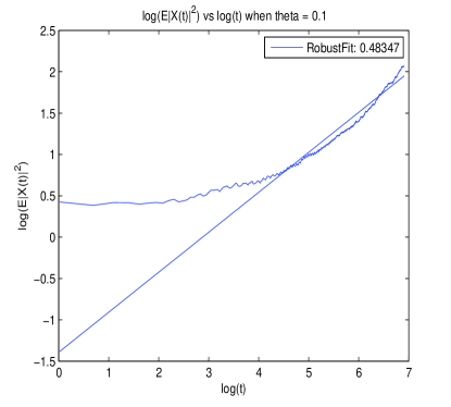
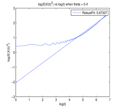
In this section, we illustrate the difference of streamline geometry and dynamical properties of steady and unsteady cellular flows. In particular, we quantify the chaotic behavior of the motion along streamlines of (1.1) using the empirical mean square distance inside infinite invariant channels in the direction , or , where denotes the particle trajectories in the flow. We show computationally that it scales with time as , , for sampled values of .
2.1 Steady Cellular Flow
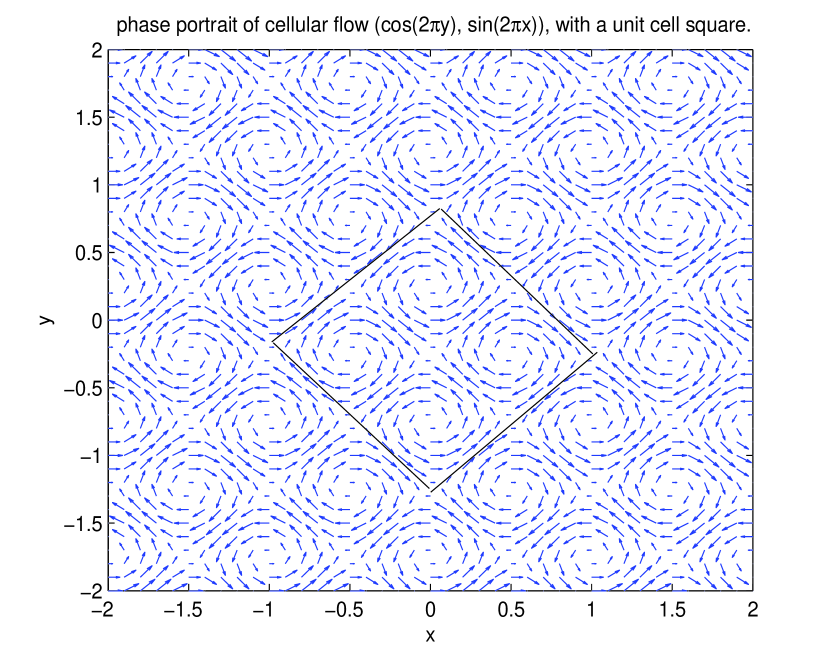
A phase portrait of the steady cellular flow
| (2.1) |
with a cell square is presented in Fig. 1. The phase portrait away from the square simply repeats. The streamlines are ordered. The closed orbits form elliptic part of the phase space. The saddles are located at half-integer points , , with connecting separatrices forming hyperbolic part of the phase space. Any particle trajectory is either a closed orbit or a separatrix, hence the motion is bounded inside the square.
2.2 Unsteady Cellular Flow
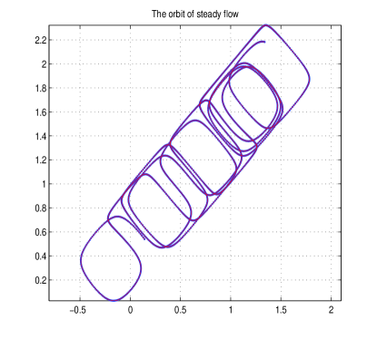
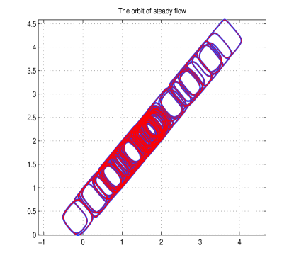
For the unsteady flow
| (2.2) |
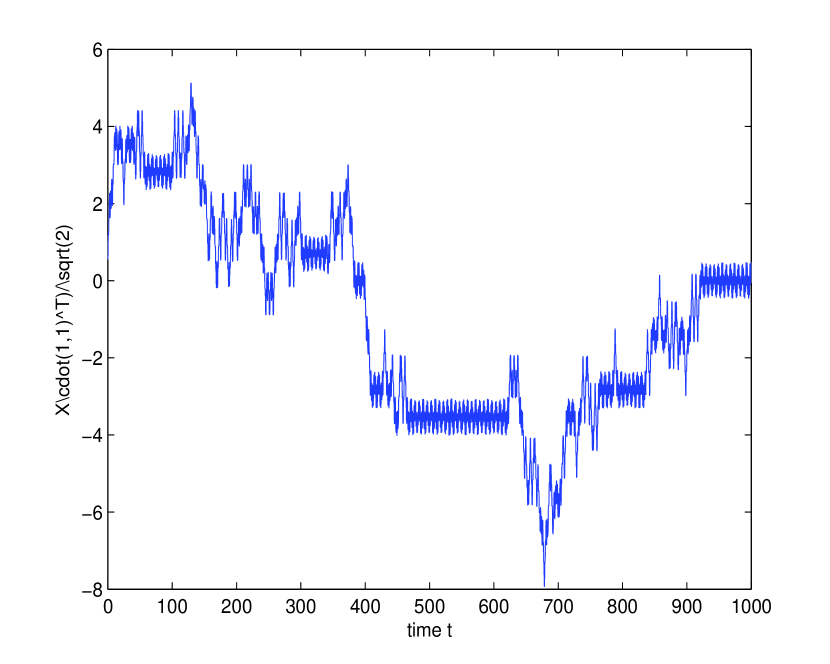
the invariant manifold consists of lines , . The flow trajectories are restricted in the channels bounded by two neighboring lines and . At , the flow trajectory extends itself from one cell square to another. The Lagrangian particle undergoes chaotic motion, see Fig. 2 for an illustration. The computation is done by a fourth order symplectic scheme. The local flow direction is colored red. The intensified red region in the middle indicates that the particle spends a lot of time wandering in and out of the cells there. Fig. 3 plots a projected trajectory in the direction vs. time. The stochastic feature is visible.
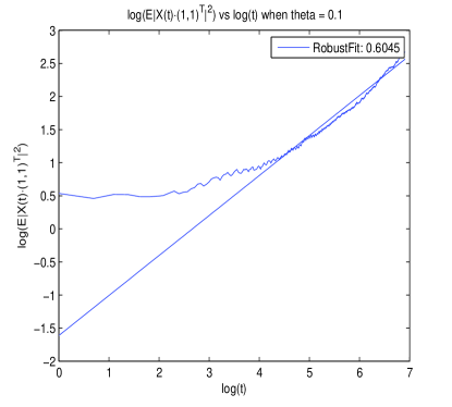
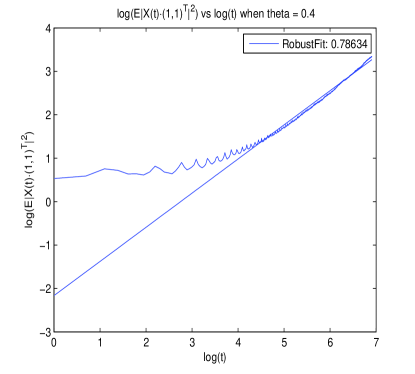
To quantify the disorder and draw a connection with diffusion process, we compute trajectories over time interval with uniformly distributed initial points on a base cell square, where denotes the random samples. We calculate the empirical mean square distance () and the projected mean square distance , and plot them as a function of time on the logarithmic scale to recover scaling laws. For efficiency, the samples are obtained by a 500 node parallel implementation of the standard 4th order Runge-Kutta method. Fig. 4 shows that the mean square distances , at respectively, hence belonging to the sub-diffusive regime. Similar sub-diffusive behavior can be observed in Fig. 5 where the projected mean square distance scales like , at .
3 Numerical Methods
Numerical approximation of advection-dominated problems is a topic of independent interest. We shall use the Edge-Averaged Finite Element (EAFE) method [31] due to the nice discrete maximum principle obeyed by EAFE and the corresponding fast multigrid solvers. On the other hand, pseudo-spectral methods are a class of highly accurate numerical methods for solving partial differential equations. In practice, pseudo-spectral method has excellent error reduction properties with the so-called “exponential convergence” being the fastest possible as long as the solution is smooth. In this section, we briefly review these two methods used in our simulation.
Recall that we are solving the following evolution problem over the unit square domain with periodic boundary condition and a constant initial condition:
| (3.1) |
3.1 EAFE Method
We first decompose the domain into a triangulation which is a set of triangles such that
| (3.2) |
For the unit square, we simply use the uniform mesh obtained by setting length of each triangle .
We describe the EAFE method using a simple advection-diffusion equation
| (3.3) |
Associated with each , let be the piecewise linear finite element space. The space is defined as the subspace of with zero trace on .
Given any edge in the triangulation, we introduce a function defined locally on (up to an arbitrary constant) by the relation:
| (3.4) |
where is the edge connecting two vertices and , and is the vector such that .
The EAFE formulation of the problem (3.3) is: Find such that
| (3.5) |
where
and
where is the angle between the edges that share the common edge and is related to the tangential derivative along .
The authors of [31] show that if the triangulation is a so-called Delaunay triangulation, i.e., the summation of two angles of an interior edge is less than or equal to , the matrix of the linear system generated by EAFE would be an M-matrix with nonnegative row sum. The detail of the scheme can be found in [31].
When applied to equation (3.1), notice that is divergence free, the operator can be written in the form of (3.3) and the reaction term is always positive. We apply the mass lumping method [26] so that the discretization of the reaction term makes positive contribution to the diagonal. Therefore the M-matrix property and consequently the discrete maximum principle still holds.
Remark 1
We have tested the Box method [5], EAFE method [31] and streamline diffusion method [11] on the advection-dominated problem. The accuracy of EAFE scheme is better than Box method, but lower than the streamline diffusion method. We chose EAFE instead of streamline diffusion scheme because the matrix of linear system generated by EAFE is M-matrix. The M-matrix not only preserves the discrete maximum principle (so that the numerical solution stays between 0 and 1) but also benefits from the fast solvers.
To accelerate the speed of computation, Algebraic Multi-Grid (AMG) solver is used to solve the linear algebraic equation arising from each time step. When the matrix is an M-matrix, the corresponding AMG solver is proven to be efficient. Specifically for the advection-diffusion equations, a multigrid method preserving the M-matrix property in coarse level is developed in [13]. Among many AMG software packages, we use AGMG (aggregation-based algebraic multigrid method) package [19]. The numerical test shows that AMG solver is times faster than the direct solver.
3.2 Pseudo-Spectral Method with Semi-Explicit Scheme
To describe the pseudo-spectral method, we consider the problem:
| (3.6) | |||
| (3.7) |
The derivatives of solutions are and . Here is the discrete Fourier transformation and represents the wave numbers.
The pseudo-spectral scheme with semi-explicit scheme is that diffusion term uses implicit scheme and advection term uses half step lagged explicit scheme:
| (3.8) |
Here the discretization on the spatial domain is and is the frequency of at time step . Pseudo-spectral method has higher order accuracy than the finite element methods. However, its time step size depends on the small diffusion parameter . Therefore it is more costly to reach the large time solution.
3.3 Stability Analysis
The pseudo-spectral method is not so efficient when diffusion parameter goes to zero. Here we compare the upwinding finite element method and pseudo-spectral method. The analysis suggests a hybrid algorithm combining finite element method and pseudo-spectral method.
3.3.1 Upwinding Finite element method
The stability condition of EAFE method is equivalent to that of an upwinding scheme. To simplify analysis, the advection term is taken as one-dimensional and the reaction term is ignored. The proto-type equation is
| (3.9) |
The upwinding semi-explicit scheme is
| (3.10) |
Denoting
we carry out the von Neumann analysis to obtain the stability condition. Upon substitution , (3.10) becomes:
| (3.11) |
Let and CFL number . The Peclet number
Equation (3.11) simplifies to:
| (3.12) |
The stable condition is:
| (3.13) |
It suffices to impose:
The stability condition of the upwinding scheme in the limit of is:
| (3.14) |
a CFL condition independent of .
3.3.2 Pseudo-Spectral Method
Consider pseudo-spectral method on the proto-type equation (3.9) again: we have shown before:
| (3.15) |
To prove the stability of pseudo-spectral method with Semi-Explicit scheme, we assume:
| (3.16) |
and we denote the projection operator:
| (3.17) |
If we plug (3.16) and (3.17) into (3.15), we have that the k-th component of the vector, which should be the corresponding coefficient of :
| (3.18) |
From (3.18), we obtain
| (3.19) |
So in (3.15) is stable if and only if:
| (3.20) |
which is equivalent to
| (3.21) |
So if the equation is advection dominant, then at least satisfies
| (3.22) |
and the stable condition would be . When , the time step is in the order of which is very restrictive.
4 Numerical Results on Residual Speeds
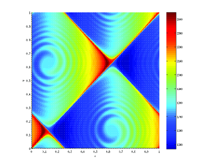
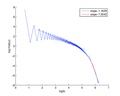
For each given , we compute the Lyapunov exponent of (1.4) by finding the long time quasi-stationary solution and applying formula (1.6). A quasi-stationary solution with is shown in the left plot of Fig. 6. The layer structure of the numerical solution moves along the direction and oscillates between the two neighboring invariant manifolds (lines of unit slope). The right plot of Fig. 6 shows the power spectrum of the auxiliary field (a genearalized eigenfunction) (right) for the unsteady flow (2.2). We observe that the energy decreases towards high frequency, with a linear decay (scaling range) in the intermediate region of wave numbers.
After calculating by the algorithm discussed in (1.6), the minimization problem (1.3) is solved by the golden-section method[4]. Golden-section method is a method to find the minimal point of a particular function called unimodal function. The idea of Golden-section method is by successively narrowing down the range of searching interval. A common definition of unimodal function is for some value , it is monotonically decreasing when and monotonically increasing when . In [18], the authors show that the function is indeed a unimodal function which is strictly convex with respect to , decreasing over interval and strictly increasing over interval , with the unique minimal point of . Notice that Newton’s method is not applicable since is not known.
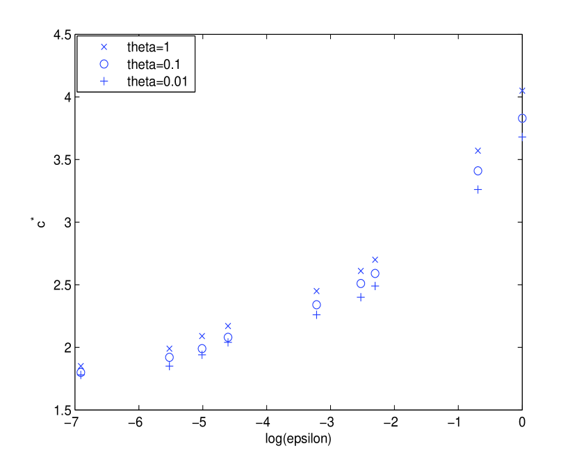
For time periodic cellular flow (1.1), EAFE method and spectral method are combined together to obtain the result in Fig. 7. The initial searching interval is . EAFE is used first to narrow down the searching interval to an neighborhood of with length 2. The space size and time step is and , respectively. Since the minimal diffusion parameter and amplitude of advection term is , the choice of leads to numerical method stable. The spectral method with space node in each direction and time step is used to obtain the minimal point when the length of searching interval is less than . The stopping criterion of searching algorithm is that the difference of two consecutive value of is less than . The benefit of using two methods together is that we can find the minimal point faster without the sacrifice of the accuracy.
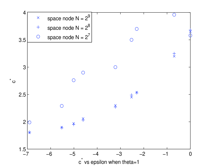
In Fig. 7, we plot as a function of for three values of parameter . Recall that is the perturbation parameter which determines how close the flow is to the steady cellular flow; see (1.1). From Fig. 7, we observe that for all three positive values of , as . In contrast, it is well known that in steady cellular flows[20]. The presence of chaotic trajectories in time periodic cellular flows contributed to this phenomenon. They are much more mobile and far reaching than their counterparts of steady cellular flows. Fig. 8 shows the persistence of residual front speeds under grid refinement at and the close proximity of the data points between those at grid sizes of and validates the convergence of the results numerically.
5 Concluding Remarks
We have studied the KPP front speed asymptotics computationally in time periodic cellular flows with chaotic streamlines in the small molecular diffusivity limit. The chaotic streamlines statistically resemble a sub-diffusion process and enhance the KPP front speed significantly in the sense that has a positive limit as molecular diffusivity tends to zero. Such residual transport phenomenon is absent in steady cellular flows with ordered streamlines. To facilitate effective computation in the advection dominated regime, we combined an upwinding finite element methods with the spectral method for computing the principal eigenvalue of a time periodic parabolic operator with small diffusion and for a subsequent minimization. In future work, we plan to study residual KPP front speeds in three space dimensional chaotic flows.
6 Acknowledgements
The work was partially supported by NSF grant DMS-1211179. We thank Tyler McMillen for helpful conversations and visualization of chaotic dynamical systems. L.C was also supported by NSF grant DMS-1115961 and DOE prime award # DE-SC0006903.
References
- [1] E. Abraham, et al., Importance of stirring in the development of an ironfertilized phytoplanton bloom, Nature 407 (2000), pp. 727–730.
- [2] M. Abel, M. Cencini, D. Vergni, A. Vulpiani, Front speed enhancement in cellular flows, Chaos 12 (2002), pp. 481–488.
- [3] B. Audoly, H. Berestycki, Y. Pomeau, Réaction diffusion en écoulement stationnaire rapide, C.R. Acad. Sci. Paris, Série IIb, 328 (2000), pp. 255–262.
- [4] R. Brent, “Algorithms for Minimization Without Derivatives”, Prentice Hall, 1973, DFMIN module http://gams.nist.gov/serve.cgi/Module/NMS/DFMIN/5671/.
- [5] R. Bank, J. Burger, W. Fichtner, R. Smith, Some upwinding techniques for finite element approximations of convection diffusion equations, Numer. Math., 58 (1990), pp. 185–202.
- [6] L. Biferale, A. Cristini, M. Vergassola, A. Vulpiani, Eddy diffusivities in scalar transport, Physics Fluids 7(11), 1995, pp. 2725–2734.
- [7] A. Brooks, T. Hughes, Streamline upwind/Petrov-Galerkin formulations for convection dominated flows with particular emphasis on the incompressible Navier-Stokes equations. Computer methods in applied mechanics and engineering 32(1), 1982, pp. 199-259.
- [8] R. Camassa, S. Wiggins, Chaotic advection in a Rayleigh-Bénard flow, Physical Review A, 43(2), 1990, pp. 774–797.
- [9] S. Childress, A. Soward, Scalar transport and alpha-effect for a family of cat’s eye flows, J. Fluid Mech. 205 (1989), pp. 99–133.
- [10] J. Cooper, J. Butcher, An Iterative Scheme for Implicit Runge-Kutta Methods, IMA J. Numer. Anal. 3, pp. 127–140, 1983.
- [11] H. Elman, D. Silvester, A. Wathen, “Finite Elements and Fast Iterative Solvers with Applications in Incompressible Fluid Dynamics”, Oxford University Press, 2005.
- [12] A. Fannjiang, G. Papanicolaou, Convection enhanced diffusion for periodic flows, SIAM J. Applied Math, 54(2), 1994, pp. 333-408.
- [13] H. Kim, J. Xu, and L. Zikatanov, A multigrid method based on graph matching for convection-diffusion equations, Numer. Linear Algebra Appl., (2003), pp. 181 – 195. More details are at: http://epubs.siam.org/doi/ref/10.1137/060659545
- [14] Y. Gorb, D. Nam, and A. Novikov, Numerical simulations of diffusion in cellular flows at high Peclet numbers, DCDS-B, vol. 51(1), 2011, pp. 75–92.
- [15] S. Heinze, Diffusion-advection in cellular flows with large Peclet numbers, Archive Rational Mech. Analysis, 168(4), 2003, pp. 329–342.
- [16] Y. Liu, J. Xin, Y. Yu, A Numerical Study of Turbulent Flame Speeds of Curvature and Strain G-equations in Cellular Flows, Physica D, 243(1), pp. 20-31, 2013.
- [17] J. Nolen, J. Xin, Asymptotic Spreading of KPP Reactive Fronts in Incompressible Space-Time Random Flows, Ann Inst. H. Poincaré, Analyse Non Lineaire, 26(3), 2009, pp. 815-839.
- [18] J. Nolen, M. Rudd, J. Xin, Existence of KPP fronts in spatially-temporally periodic advection and variational principle for propagation speeds, Dynamics of PDE, 2(1), pp. 1-24, 2005.
- [19] Y. Notay, AGMG software and documentation; see http://homepages.ulb.ac.be/ ynotay/AGMG
- [20] A. Novikov, L. Ryzhik, Boundary layers and KPP fronts in a cellular flow, Arch. Ration. Mech. Anal., 184(1), 2007, pp. 23 – 48.
- [21] M. Paoletti, T. Solomon, Experimental studies of front propagation and mode-locking in an advection-reaction-diffusion system, Europhys. Lett. 69 (2005), pp. 819–825.
- [22] P. Ronney, Some Open Issues in Premixed Turbulent Combustion, Modeling in Combustion Science (J. D. Buckmaster and T. Takeno, Eds.), Lecture Notes In Physics, Vol. 449, Springer-Verlag, Berlin, 1995, pp. 3-22.
- [23] L. Ryzhik, A. Zlatos, KPP pulsating front speed-up by flows, Commun. Math. Sci. 5 (2007), pp. 575–593.
- [24] W. van Saarloos, Front propagation into unstable states, Physics Reports 386(2), 2003, pp. 29-222.
- [25] L. Shen, A. Zhou, J. Xin, Finite Element Computation of KPP Front Speeds in Cellular and Cat’s Eye Flows, Journal of Scientific Computing, 55(2), 2013, pp. 455–470.
- [26] P. Tong, T.H.H. Pian, L.L. Bucciarelli, Mode shapes and frequencies by finite element method using consistent and lumped masses, Comput. Struct. 1 (1971), pp. 623-638.
- [27] F. Williams, “Combustion Theory”, Benjamin-Cummings, Menlo Park, 1985.
- [28] J. Xin, “An Introduction to Fronts in Random Media”, Surveys and Tutorials in Applied Math Sciences, Vol. 5, Springer, 2009.
- [29] J. Xin, Y. Yu, Front Quenching in G-equation Model Induced by Straining of Cellular Flow, Arch. Rational Mechanics Analysis, to appear.
- [30] J. Xin, Y. Yu, Asymptotic growth rates and strong bending of turbulent flame speeds of G-equation in steady two dimensional incompressible periodic flows, SIAM J. Math Analysis, to appear.
- [31] J. Xu, L. Zikatanov, A monotone finite element scheme for convection diffusion equations, Math. Comp., 68 (1999), pp. 1429–1446.