Corrections to Eikonal Approximation for Nuclear Scattering at Medium Energies

Abstract

The upcoming Facility for Rare Isotope Beams (FRIB) at the National Superconducting Cyclotron Laboratory (NSCL) at Michigan State University has reemphasized the importance of accurate modeling of low energy nucleus-nucleus scattering. Such calculations have been simplified by using the eikonal approximation. As a high energy approximation, however, its accuracy suffers for the medium energy beams that are of current experimental interest. A prescription developed by Wallace Wallace:1971zz ; Wallace:1973iu that obtains the scattering propagator as an expansion around the eikonal propagator (Glauber approach) has the potential to extend the range of validity of the approximation to lower energies. Here we examine the properties of this expansion, and calculate the first-, second-, and third-order corrections for the scattering of a spinless particle off of a ⁴⁰Ca nucleus, and for nuclear breakup reactions involving ¹¹Be. We find that, including these corrections extends the lower bound of the range of validity of the down to energies of 40 MeV. At that energy the corrections provide as much as a 15% correction to certain processes.

I Introduction

Ongoing and planned experiments using rare isotopes promise to further our understanding of nuclei and their role in astrophysics msu . Nuclear reaction theory is needed both to interpret the data and to determine the necessary experiments Hansen:2003sn ; gg08 ; Bertulani:2009mf . Use of the eikonal approximation (also known as Glauber theory roy ) has long been known as appealing procedure to simplify the calculations, for medium and low energies see e.g. Bertsch:1990zz ; Ogawa:1992tf ; AlKhalili:1996zz ; Hencken:1996af ; Aumann:2000zz . This technique has often been used to analyze experiments, see e.g Parfenova:2000be ; Licot:1997zz ; Sauvan:2000hq performed at energies less than 100 MeV per nucleon. A computer program using the eikonal approximation, described as being appropriate for knockout reactions for energies between 30 and 2000 MeV per nucleon, has been published Bertulani:2006fe . However, as stated in the orignal article roy the Glauber theory rests on the approximation that the product of the wave number $k$ and the range of the relevant potential $a$ satisfy

$$k\,a\gg 1$$ (1)

and that the magnitude of the scattering potential $V$ be very small compared to the scattering energy, $E$, so that

$$V/E\ll 1.$$ (2)

For a nucleon of energy 100 MeV and nucleus of radius $\approx 3$ fm, $k\,a\approx 6$, and $V/E\approx 1/2.$ It is far from obvious that the conditions for the accuracy of the Glauber approximation are satisfied. Moreover, it is not clear if the relevant distance appearing in the term $ka$ should be the nuclear radius or the nuclear diffuseness. If the latter, the beam energy must be higher for the eikonal approximation to be valid. It is therefore of interest to assess the accuracy of Glauber theory and the lower limits on energy for which it may be applied Esbensen:2001mr . In the following we treat the terms eikonal approximation and Glauber theory as synonymous.

The conclusions of Ref. Esbensen:2001mr have been summarized Hansen:2003sn as showing that the eikonal approximation is accurate to within a few percent for energies as low as 20 MeV/nucleon. This conclusion is based on a comparison between the results of using the eikonal approximation and a time-dependent Schrödinger equation. The incoming projectile is treated as a bound state of a nucleon and a core. The time-dependent Schrödinger equation that includes the dynamics of the interaction of the nucleon with the core as well as the nucleon-target interaction was solved. We do not believe the conclusion that the eikonal approximation is valid at 20 MeV Hansen:2003sn to be a valid summary of the work of Ref. Esbensen:2001mr . This is because the time-dependent equation (their Eqs.(5,6)) treats the motion of the core of the projectile as following the linear trajectory ${\bf R}={\bf b}+{\bf v}t$. In other words, the eikonal approximation is used in the time-dependent Schroedinger equation. Thus the work contains no actual test of the eikonal approximation. However, Ref. Esbensen:2001mr does have the very useful result that the interaction between the nucleon and the core that occurs during the nuclear reaction can be neglected for energies as low as 20 MeV/nucleon. Thus the so-called sudden approximation is justified, at least for one particular state. However, the use of the eikonal approximation has not been justified and the range of its validity has not been fully determined. Thus the present paper is devoted to studying the corrections to the eikonal approximation.

In this paper we assess the validity of the eikonal approximation by computing the corrections Sect. II to this approximation for potential scattering Sect. III, and for reactions involving halo nuclei Sect. IV. The principal tool is the expansion developed by Wallace Wallace:1971zz ; Wallace:1973iu in which the complete Green’s function is expanded about the Glauber approximation to the complete Green’s function. Our results and directions for further research are summarized in a final Sect. V.

II Corrections to the Eikonal Theory

We first apply the corrections to the eikonal approximation described by Wallace Wallace:1971zz ; Wallace:1973iu for scattering of a spin-zero particle off a generic potential. This exercise is useful because we can calculate the scattering amplitude exactly using a partial wave expansion and compare it with successive corrections in the eikonal expansion. We will give a quick review of the corrections here using the same notation as Wallace:1971zz ; Wallace:1973iu before showing the results of our calculations.

The $T$ matrix for scattering at a center of mass energy $E=K^{2}/2M$ is given by

$$T(E)=V+VG_{0}(E)T=V+VG(E)T(E),$$ (3)

where $G^{-1}(E)=E-P^{2}/2M-V+i\epsilon$ is the particle propagator and $V$ is the interaction potential.

The Wallace eikonal expansion consists of expanding the momentum operator $\mathbf{P}$ about a particular vector $\mathbf{k}$ and dropping all terms quadratic in ${\bf P}-\mathbf{k}$. The choice ${\bf k}=K\widehat{{\bf k}}$ with $\widehat{{\bf k}}$ as the average of the projectile initial and final direction ($\mathbf{k}=(\mathbf{k}_{i}+\mathbf{k}_{f})/2$) gives the Glauber approximation and the propagator:

$$g^{-1}=\mathbf{v}\cdot(\mathbf{k}-\mathbf{P})-V+i\epsilon.$$ (4)

The difference between the full propagator $G$ and the reduced eikonal propagator $g$ is given by

$$g^{-1}-G^{-1}=N$$ (5)

$$N=(1-\cos(\theta/2))(g^{-1}+V)+[(\mathbf{P}-\mathbf{k}_{f})\cdot(\mathbf{P}-\mathbf{k}_{i})]/2M,$$ (6)

where $\theta$ is the scattering angle.

It is then possible to solve for the $T$ matrix as a perturbation series:

$$T=(V+VgV)+VgNgV+VgNgNgV+VgNgNgNgV+\dots.$$ (7)

The Glauber approximation consists of keeping only the terms in parentheses, and Wallace showed how to systematically calculate higher order correction terms. The result is an expansion in powers of the interaction energy over the kinetic energy with corrections due to the spatial non-uniformity of the potential. He explicitly calculates the first three correction terms, and first with the conjecture of some advantageous cancellations Wallace:1971zz ; Wallace:1973iu , and later Wallace:1973ni in an explicit calculation obtained the following expressions:

$$T^{(0)}(\mathbf{b}) =e^{i\chi_{0}(|\mathbf{b}|)}-1$$ (8)

$$T^{(1)}(\mathbf{b}) =e^{i(\chi_{0}(|\mathbf{b}|)+\tau_{1}(|\mathbf{b}|))}-1$$ (9)

$$T^{(2)}(\mathbf{b}) =e^{i(\chi_{0}(|\mathbf{b}|)+\tau_{1}(|\mathbf{b}|)+\tau_{2}(|\mathbf{b}|))}e^{-\omega_{2}(|\mathbf{b}|)}-1$$ (10)

$$T^{(3)}(\mathbf{b}) =e^{i(\chi_{0}(|\mathbf{b}|)+\tau_{1}(|\mathbf{b}|)+\tau_{2}(|\mathbf{b}|)+\tau_{3}(|\mathbf{b}|)+\phi_{3}(|\mathbf{b}|))}e^{-\omega_{2}(|\mathbf{b}|)-\omega_{3}(|\mathbf{b}|)}-1.$$ (11)

Here $\mathbf{b}$ is the impact parameter, $T^{(0)}$ is the Glauber approximation, and the phases are defined below, with $\mathbf{z}\perp\mathbf{b}$, $\mathbf{r}=\mathbf{b}+\mathbf{z}$, $U(r)=V(r)/V(0)$, $\widehat{\beta}_{n}\equiv b^{n}\partial^{n}/\partial b^{n}$, and $\epsilon=V(0)/2E$:

$$\chi_{0}(b) =-2K\epsilon\int_{0}^{\infty}\!\mathrm{d}z\,U(r)$$ (12)

$$\tau_{1}(b) =-K\epsilon^{2}(1+\widehat{\beta}_{1})\int_{0}^{\infty}\!\mathrm{d}z\,U^{2}(r)$$ (13)

$$\tau_{2}(b) =-K\epsilon^{3}(1+\frac{5}{3}\widehat{\beta}_{1}+\frac{1}{3}\widehat{\beta}_{2})\int_{0}^{\infty}\!\mathrm{d}z\,U^{3}(r)-\frac{b[\chi_{0}^{\prime}(b)]^{3}}{24K^{2}}$$ (14)

$$\omega_{2}(b) =b\chi_{0}^{\prime}(b)\frac{\nabla^{2}\chi_{0}(b)}{8K^{2}}$$ (15)

$$\tau_{3}(b) =-K\epsilon^{4}(\frac{5}{4}+\frac{11}{4}\widehat{\beta}_{1}+\widehat{\beta}_{2}+\frac{1}{12}\widehat{\beta}_{3})\int_{0}^{\infty}\!\mathrm{d}z\,U^{4}(r)-\frac{b\tau_{1}^{\prime}(b)[\chi_{0}^{\prime}(b)]^{2}}{8K^{2}}$$ (16)

$$\phi_{3}(b) =-K\epsilon^{2}(1+\frac{5}{3}\widehat{\beta}_{1}+\frac{1}{3}\widehat{\beta}_{2})\int_{0}^{\infty}\!\mathrm{d}z\,\left[\frac{\partial U(r)/\partial r}{2K}\right]^{2}$$ (17)

$$\omega_{3}(b) =\frac{b\chi_{0}^{\prime}(b)\nabla^{2}\tau_{1}(b)+b\tau_{1}^{\prime}(b)\nabla^{2}\chi_{0}(b)}{8K^{2}}$$ (18)

We see that the corrections related to $\widehat{\beta}_{n}$ involve the derivatives of the nuclear potential which are large in the region of the nuclear surface. This indicates that the product of the wave number and the nuclear diffuseness parameter, needs to be large compared to unity for the eikonal approximation to be valid. This condition is more stringent than the one involving the product of the wave number and the nuclear radius.

The scattering amplitude is then simply:

$$f(\mathbf{q})=-iK/2\int\!\mathrm{d^{2}}b\,e^{i{\bf q\cdot b}}T^{(n)}(\mathbf{b}).$$ (19)

III Eikonal Expansion vs. Exact Partial Wave Results

Our focus is on reactions at FRIB energies. We therefore evaluate the scattering amplitude for protons scattering off of ⁴⁰Ca using the potential described by Varner et. al. Varner:1991zz for incident center-of-mass kinetic energy between 16 and 98 MeV. We neglect the spin-orbit and the Coulomb interaction because such terms are neglected in Ref. Hencken:1996af .

This potential is then given by

$$V(r,E)=-V_{r}(E)\,f_{\rm ws}(r,R_{0},a_{0})-iW_{\rm v}(E)\,f_{\rm ws}(r,R_{\rm w},a_{\rm w})-i\,W_{\rm s}(E){d\over dr}\,f_{\rm ws}(r,R_{\rm w},a_{\rm w}),$$ (20)

with

$$f_{\rm ws}(r,R,a) = {1\over 1+\exp[(r-R)/a]}$$ (21)

$$V_{r}(E) = V_{0}+V_{\mathrm{e}}(E-E_{\mathrm{c}})\pm V_{\rm t}\varepsilon$$ (22)

$$W_{\mathrm{v}}(E) = W_{\rm v0}f_{\mathrm{ws}}(W_{\mathrm{ve0}},(E-E_{\mathrm{c}}),W_{\mathrm{vew}})$$ (23)

$$W_{\mathrm{s}}(E) = (W_{\rm s0}\pm W_{\rm st}\varepsilon)f_{\mathrm{ws}}((E-E_{\mathrm{c}}),W_{\mathrm{se0}},W_{\mathrm{sew}}),$$ (24)

where the $\pm$ indicates $+$ for proton projectiles and $-$ for neutron projectiles. Parameters in the model can be found in Table 1 and in the text.

Parameter	Value	Uncertainty
$\varepsilon$	$(N-Z)/A$	–
$V_{0}$	52.9 MeV	$\pm~{}0.2$
$V_{\rm t}$	13.1 MeV	$\pm~{}0.8$
$V_{\rm e}$	-0.299	$\pm~{}0.004$
$r_{0}$	1.250 fm	$\pm~{}0.002$
$r_{0}^{(0)}$	-0.225 fm	$\pm~{}0.009$
$R_{0}$	$r_{0}A^{1/3}+r_{0}^{(0)}$	–
$a_{0}$	0.690 fm	$\pm~{}0.006$
$r_{\rm c}$	1.24 fm	–
$r_{\rm c}^{(0)}$	0.12 fm	–
$R_{\rm c}$	$r_{\rm c}A^{1/3}+r_{\rm c}^{(0)}$ fm	–
$E_{\mathrm{c}}$	$6Ze^{2}/5R_{\mathrm{c}}$ MeV	–
$W_{\rm v0}$	7.8 MeV	$\pm~{}0.3$
$W_{\rm ve0}$	35 MeV	$\pm~{}1$
$W_{\rm vew}$	16 MeV	$\pm~{}1$
$W_{\rm s0}$	10.0 MeV	$\pm~{}0.2$
$W_{\rm st}$	18 MeV	$\pm~{}1$
$W_{\rm se0}$	36 MeV	$\pm~{}2$
$W_{\rm sew}$	37 MeV	$\pm~{}2$
$r_{\rm w}$	1.33 fm	$\pm~{}0.01$
$r_{\rm w}^{(0)}$	-0.42 fm	$\pm~{}0.03$
$R_{\rm w}$	$r_{\rm w}A^{1/3}+r_{\rm w}^{(0)}$ fm	–
$a_{\rm w}$	0.69 fm	$\pm~{}0.01$

Table 1: Parameters of interest from ref Varner:1991zz

The approximate eikonal solution to potential scattering can be compared with an exact solution obtained by using a partial wave technique. Phase shifts for arbitrary values of $\ell$ are obtained by numerically solving the radial Schrödinger equation,

$$\frac{d^{2}u_{\ell}}{dr^{2}}+\left(k^{2}-2mV-\frac{\ell(\ell+1)}{r^{2}}\right)u_{\ell}=0,$$

matching $u_{\ell}(R)=Re^{i\delta_{\ell}}[\cos(\delta_{\ell})j_{\ell}(kR)-\sin(\delta_{\ell})n_{\ell}(kR)]$ for $R$ large enough such that $V(R)\approx 0$, and solving for $\delta_{\ell}$. Here, $j_{\ell}$ and $n_{\ell}$ are spherical Bessel functions of the first and second kind, respectively. The scattering amplitude is then:

$$f(\theta)=\sum_{\ell=0}^{\infty}(2\ell+1)e^{i\delta_{\ell}}\sin\delta_{\ell}P_{\ell}(\cos\theta).$$

This sum is taken to convergence and compared to scattering amplitudes derived from the eikonal approximation. This comparison provides an indication of the validity of the approximation when applied to more complex systems for which an exact solution is not feasible.

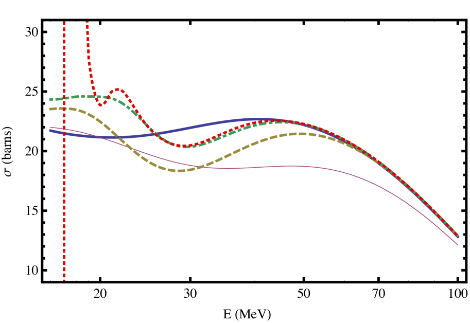
Figure 1: (Color online) Total nuclear cross-section $\sigma$ for a proton incident on ⁴⁰Ca as a function of beam energy. The exact partial wave result is the thick blue line, the zeroth-order eikonal approximation is the thin magenta line, the first-order eikonal approximation is the beige dashed line, the second-order eikonal approximation is the green dot-dashed line, and the third-order eikonal approximation is the red dotted line.

III.1 Results of Calculations

Our main results for these calculations are presented in figures 1-4. Figure 1 shows the total elastic nuclear cross-section of a spinless proton incident on a ⁴⁰Ca nuclear potential in the exact calculation, and in successive orders in the eikonal expansion. The zeroth order eikonal approximation has an error of at least 5% up to 100 MeV, while including the correction terms reduces the error to $<$ 1% above about 45 MeV. The relative degree of agreement between the zeroth order approximation and the exact calculation at energies below 20 MeV is likely a coincidence.

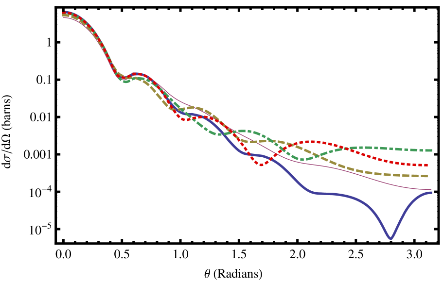
Figure 2: (Color online) Differential elastic cross-section $d\sigma/d\Omega$ for p + ⁴⁰Ca at a beam energy of 40 MeV in log scale. The angle $\theta$ is the scattering angle from the forward direction. The designations for the lines are the same as in Fig. 1.

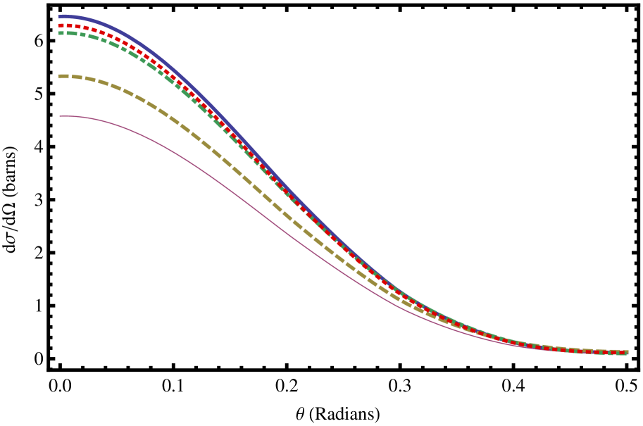
Figure 3: (Color online) Same as Fig. 2, but zoomed in on the forward scattering region, and with a linear scale.

Figures 2 and 3 show the differential elastic cross-section for the same reaction at a beam energy of 40 MeV. Even for forward scattering, the zeroth-order eikonal approximation severly underestimates the exact value, and successive corrections monotonically improve the estimate. The corrections also successively improve the range in the polar angle $\theta$ over which the approximation is accurate.

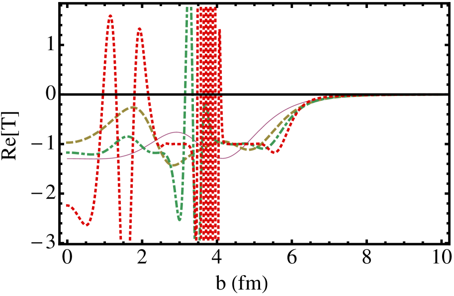
(a) Beam Energy at 20 MeV

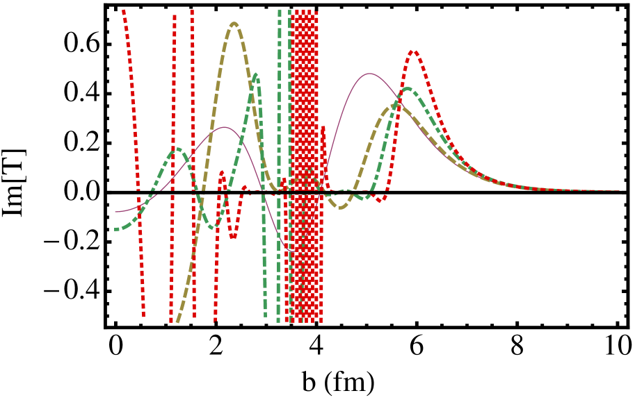
(b) Beam Energy at 20 MeV

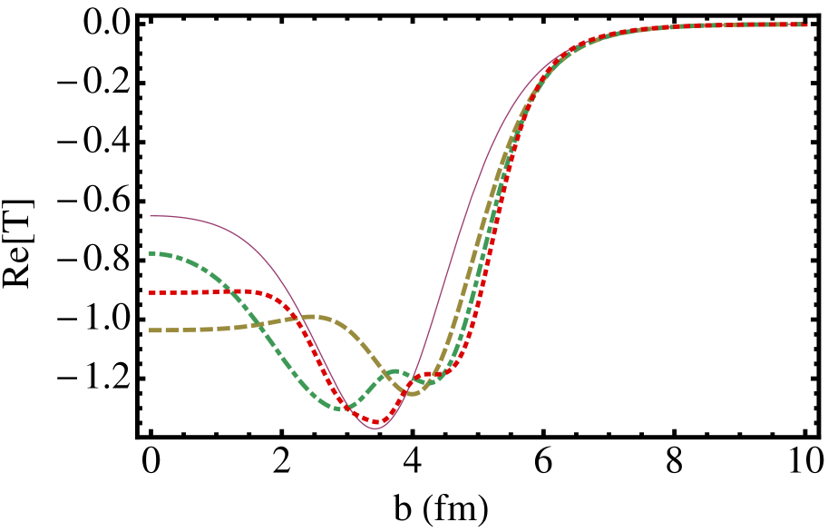
(c) Beam Energy at 40 MeV

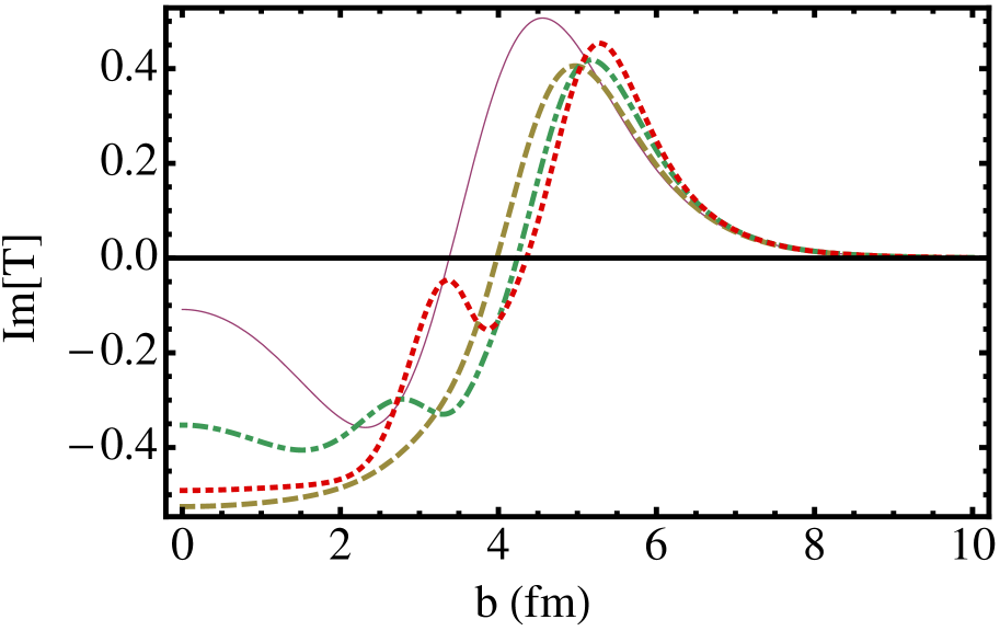
(d) Beam Energy at 40 MeV

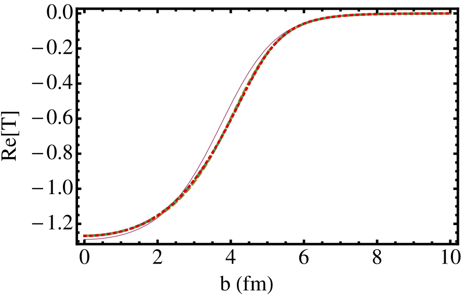
(e) Beam Energy at 98 MeV

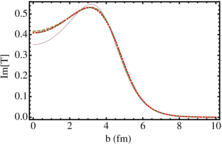
(f) Beam Energy at 98 MeV

Figure 4: (Color online) Real and imaginary parts of the transition matrix elements $T^{(n)}(b)$ for successive orders $n$ in the eikonal expansion. The designations for the lines are the same as in figs. 1.

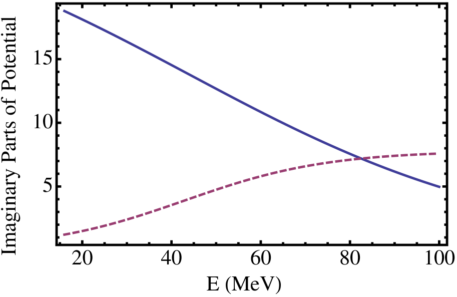
(a) Imaginary surface (solid blue) $W_{\rm s}(E)$ and volume (dashed magenta) $W_{\rm v}(E)$ terms of Varner potential as a function of beam energy.

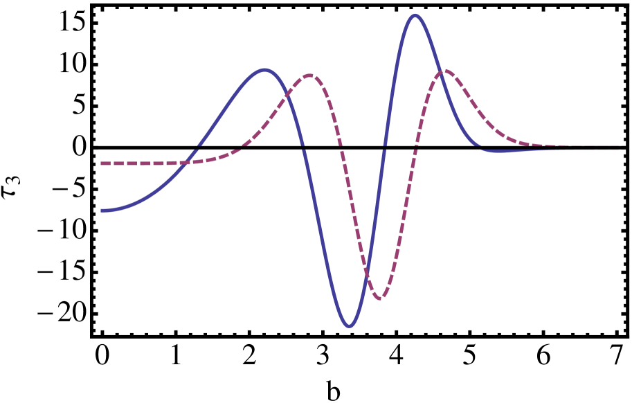
(b) Real (solid blue) and imaginary (dashed magenta) parts of $\tau_{3}(b)$ at a beam energy of 20 MeV.

Figure 5: (Color online)

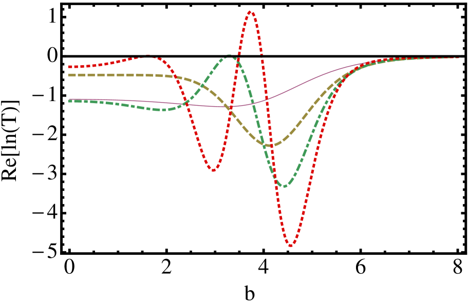
(a)

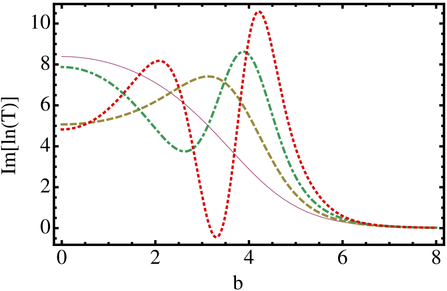
(b)

Figure 6: (Color online) Real and imaginary parts of $\ln(T^{(n)}(b))$ for $n=0$ (thin magenta), $n=1$ (dashed beige), $n=2$ (dot-dashed green), and $n=3$ (dotted red) calculated at a beam energy of 25 MeV.

Figure 4 gives the real and imaginary parts of the $T$-matrix elements $T^{(n)}(b)$ for successive orders $n$ in the expansion as a function of the impact parameter $b$ at a variety of beam energies. The rapid oscillations and drastic changes in $T$ with each correction at 20 MeV imply that the expansion is not appropriate there. This is because the interaction potential is energy dependent. In this case, it is the imaginary part of the potential that is important. It has both a surface and a volume term which have magnitudes that behave oppositely as a function of beam energy, as shown in fig. 5(a). At low energies, the surface term dominates and the derivative operators $\widehat{\beta}_{n}$ in $\tau_{3}(b)$ are large, negative, and imaginary, (see Fig. 5(b)) which generate large oscillations in $T^{(3)}(b)$. (The frequencies of such oscillations are given by the real part of $\tau_{3}(b)$.) This behavior also occurs in $\tau_{2}(b)$ and $\tau_{1}(b)$, but at lower energies. The point at which this breakdown occurs provides a lower bound on the effectiveness of the expansion that can be computed order-by-order. For example, in fig. 6(a), which was calculated at 25 MeV, the third-order correction has a real part of about 1, which is already an amplitude of oscillations in $T^{(3)}(b)$ of about 2.7 at $b\approx 3.75$. The second-order correction is about to enter positive territory in fig. 6(a) at $b\approx 3.25$, and will start to generate similar rapid oscillations in $T^{(2)}(3.25)$ at lower eneries. This can be seen in fig. 4(a), which was calculated at 20 MeV. Thus, empirically, the second-order correction is effective to about 25 MeV for this potential. Using the same method, we find the third-order correction to be effective to about 30 MeV.

Since the convergence of the expansion improves at higher energies, calculating only the first-order correction should be sufficient at some sufficiently high beam energy. From fig. 1 this appears to happen for this potential at a beam energy of about 60 MeV. Above this value, the fractional error in the second- and third-order corrections is only marginally lower than the fractional error in the first-order correction.

With these calculations, it is apparent that for at least some interactions, these corrections to the eikonal approximation are meaningful over a range of energies. It is therefore worthwhile to apply the corrections to a more interesting interaction to further evaluate their effectiveness.

IV Breakup Reactions of Halo Nuclei ¹¹Be

We now apply these calculations to the study of scattering of ¹¹Be off of various targets, using the reaction theory of Hencken, Bertsch & Esbensen Hencken:1996af . They computed the diffractive, neutron stripping, core stripping, and total absorption cross sections for ¹¹Be scattered off targets with mass number ranging from 9-208 using the Glauber eikonal approximation at an energy of 40 MeV/nucleon. They used the Varner potential Varner:1991zz as the model for nucleon-nucleon scattering. Given that we see a significant improvement in the performance of the eikonal approximation at that energy when the Wallace corrections are included for the Varner potential, it is fruitful to investigate whether or not the cross-sections evaluated by Hencken and Bertsch also experience similar improvement.

The relevant formulae of Ref. Hencken:1996af are displayed next. The reaction considered is $H+T\rightarrow c+X$, where the projectile halo nucleus $H$ is treated in a single particle model as $c+n$ with $c$ corresponding to a specific final state of the core. The halo nuclear ground state is described by a wave function $\phi_{LM}({\bf r})$ which depends on the relative coordinate $\vec{r}$ between the nucleon and the core, see Fig. 7. The function is generally specified by $\phi_{LM}({\bf r})=R_{L}(r)Y_{LM}(\widehat{{\bf r}})$ where $Y_{LM}(\widehat{{\bf r}})$ are spherical harmonics. Here we take $R_{L}(r)$ to be the solution to the radial Schrödinger equation in an $L=0$ state with the appropriate binding energy of 0.503 MeV.

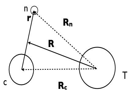
Figure 7: Coordinates used in this calculation. ${\bf R}$ is the coordinate of the center of mass of the halo nucleus, and ${\bf b}_{c}$ and ${\bf b}_{n}$ denote the components of $\mathbf{R}_{c}$ and $\mathbf{R}_{n}$ that are transverse to the beam direction.

The scattering wave function of the halo nucleus has the form,

$$\Psi({\bf r},{\bf R})=S_{n}({\bf b}_{n})S_{c}({\bf b}_{c})\phi_{LM}({\bf r})\ ,$$ (25)

in its rest frame, where (Fig. 7) ${\bf R}$ is the coordinate of the center of mass of the halo nucleus, and ${\bf b}_{c}$ and ${\bf b}_{n}$ are the impact parameters of the core and the nucleon with respect to the target nucleus, i. e. ${\bf b}_{n}={\bf R}_{\perp}+{\bf r}_{\perp}A_{c}/(A_{c}+1)$ and ${\bf b}_{c}={\bf R}_{\perp}-{\bf r}_{\perp}/(A_{c}+1)$, where $A_{c}$ is the mass number of the core and the designation $\perp$ refers to components transverse to ${\bf R}_{n}$ and ${\bf R}_{c}$. The two profile functions, $S_{n}({\bf b}_{n})$ for the nucleon and $S_{c}({\bf b}_{c})$ for the core, are generated by interactions with the target nucleus. In the eikonal approximation, they are defined by the longitudinal integrals over the corresponding potentials:

$$S({\bf b})=\exp\left[\frac{-i}{\hbar v}\int dzV({\bf b}+z\widehat{z})\right]\ ,$$ (26)

where $v$ is the beam velocity and potential $V$ is the optical potential. The relation between $S({\bf b})$ and the quantities denoted as $T({\bf b})$ of Sect. II) is given by

$$S({\bf b})=T({\bf b})+1.$$ (27)

We compute the order $n$ corrections by replacing $S({\bf b})$ from equation 26 with $T^{(n)}({\bf b})+1$ from equations 18.

The scattering wave function is the difference between eq. (25) and the wave function of the undisturbed beam,

$$\Psi_{scat}=(S_{n}S_{c}-1)\phi_{LM}\ .$$ (28)

with the shorthand notation $S_{n}=S_{n}(\mathbf{b_{n}})$ and $S_{c}=S_{c}(\mathbf{b_{c}})$.

Scattering cross sections are calculated by taking overlaps of $\Psi_{scat}$ with different final states. For diffractive breakup the final state depends on the relative momentum $\vec{k}$ of nucleon and core in their center-of-mass frame as well as on the transverse momentum $\vec{K}_{\perp}$ of the center of mass. Writing the continuum nucleon-core wave function as $\phi_{{\bf k}}(\vec{r})$ (normalized asymptotically to a plane wave: $\phi_{\bf k}\sim\exp(i{\bf k}\cdot{\bf r})$) the diffractive breakup cross section is given by

$$\frac{d\sigma_{\text{diff.}}}{\left(d^{2}\ {K}_{\perp}d^{3}{k}\right)}=\frac{1}{(2\pi)^{5}}\frac{1}{2L+1}\sum_{M}\left|\int d^{3}{r}d^{2}{R}_{\perp}e^{-i{\bf K}_{\perp}\cdot{{\bf R}}_{\perp}}\phi_{{\bf k}}^{*}({\bf r})S_{c}S_{n}\phi_{LM}({\bf r})\right|^{2}\ .$$ (29)

To obtain the relative momentum distribution in $\vec{k}$, integrate over ${\bf K}_{\perp}$ to get

$$\frac{d\sigma_{\text{diff.}}}{d^{3}{k}} = \frac{1}{(2\pi)^{3}}\frac{1}{2L+1}\sum_{M}\int d^{2}{R}_{\perp}\left|\int d^{3}{r}\phi_{{\bf k}}^{*}({\bf r})S_{c}S_{n}\phi_{L,M}({\bf r})\right|^{2}\ .$$ (30)

A convenient expression for the total diffractive cross section can be derived using completeness if $\phi_{LM}$ is the only bound state of the system. The result is

$$\sigma_{\text{diff.}} = \frac{1}{2L+1}\sum_{M}\int d^{2}{R}_{\perp}\Bigg{[}\int d^{3}\vec{r}\phi_{L,M}({\bf r})^{*}\left|S_{c}S_{n}\right|^{2}\phi_{L,M}({\bf r})-\sum_{M}\left|\int d^{3}r\phi_{0,M_{0}^{\prime}}({\bf r})^{*}S_{c}S_{n}\phi_{L,M}({\bf r})\right|^{2}\Bigg{]}\ .$$

Other contributions to the total cross section come from absorption, present when the eikonal $S$-factors have moduli less than 1. There are three of these so-called stripping processes. The nucleon-absorption cross section, differential in the momentum of the core, is given by

$$\frac{d\sigma_{\text{n-str.}}}{d^{3}{k}_{c}} = \frac{1}{(2\pi)^{3}}\frac{1}{2L+1}\sum_{M}\int d^{2}{b}_{n}\left[1-\left|S_{n}({\bf b}_{n})\right|^{2}\right]\times\left|\int d^{3}{\bf r}e^{-i{\bf k}_{c}\cdot{\bf r}}S_{c}({\bf b}_{c})\phi_{L,M}({\bf r})\right|^{2}\ .$$ (32)

The corresponding total cross section for stripping of the nucleon is

$$\sigma_{\text{n-str.}} = \frac{1}{2L+1}\sum_{M}\int d^{2}{b}_{n}\left[1-\left|S_{n}({\bf b}_{n})\right|^{2}\right]\int d^{3}{\bf r}\phi_{L,M}({\bf r})^{*}\left|S_{c}({\bf b}_{c})\right|^{2}\phi_{L,M}({\bf r})\ .$$ (33)

The stripping of the core is expressed in a similar way, interchanging subscripts $n$ and $c$.

The expression for absorption of both nucleon and core is given by

$$\sigma_{\text{abs.}} = \frac{1}{2L+1}\sum_{M}\int d^{2}{b}_{c}\left[1-\left|S_{c}({\bf b}_{c})\right|^{2}\right]\times\int d^{3}\vec{r}\phi^{*}_{L,M}({\bf r})\left[1-\left|S_{n}({\bf b}_{n})\right|^{2}\right]\phi_{L,M}({\bf r})\ .$$ (34)

IV.1 The potential for the Nucleon-Target and Core-Target Interaction

Evaluation of the profile functions requires a potential model for the interaction between the target nucleus and the constituents of the halo nucleus. At low energies, extending up to about 100 MeV/$n$, one can find optical potentials that are fit to nucleon-nucleus scattering. We use the optical potential, $V_{\rm op}$ of ref. Varner:1991zz , which was fit to scattering data in the range of 10 to 60 MeV. The potential has the usual Woods-Saxon form, with volume and surface imaginary terms, but we neglect the spin-orbit and Coulomb interactions as does Hencken:1996af . This potential represents the target-nucleon interaction. The core-target interaction potential is obtained by folding $V_{\rm op}$ with the core density distribution,

$$V_{c}(r)=\int d^{3}{x}\rho_{c}(x)V_{\text{op}}(\left|{\bf r}-\bf{x}\right|)\ .$$ (35)

For the core density we use a harmonic oscillator density with parameters taken from the charge distribution of the core nucleus devries87 ($a$=2.5 fm and $\alpha$=0.61).

IV.2 Results of Eikonal Expansion Calculations

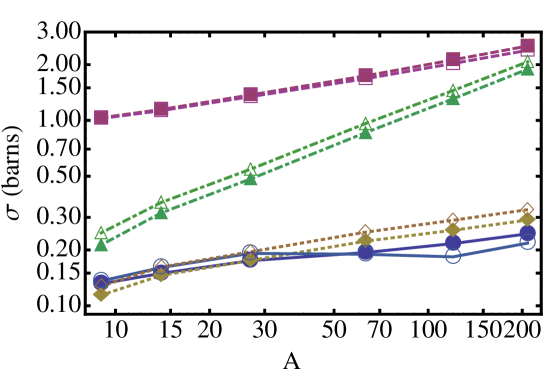
Figure 8: (Color online) Comparison of first-order corrections with standard (zeroth-order) eikonal approximation with a beam energy of 40 MeV/nucleon. The zeroth-order terms are shown with solid markers, and the first-order terms are with outlined markers. The solid (blue) line with circles is diffractive scattering, the dashed (magenta) line with squares is core stripping, the dotted (beige) line with diamonds is neutron stripping, and the dash-dotted (green) line with triangles is total absorption of the core and neutron.

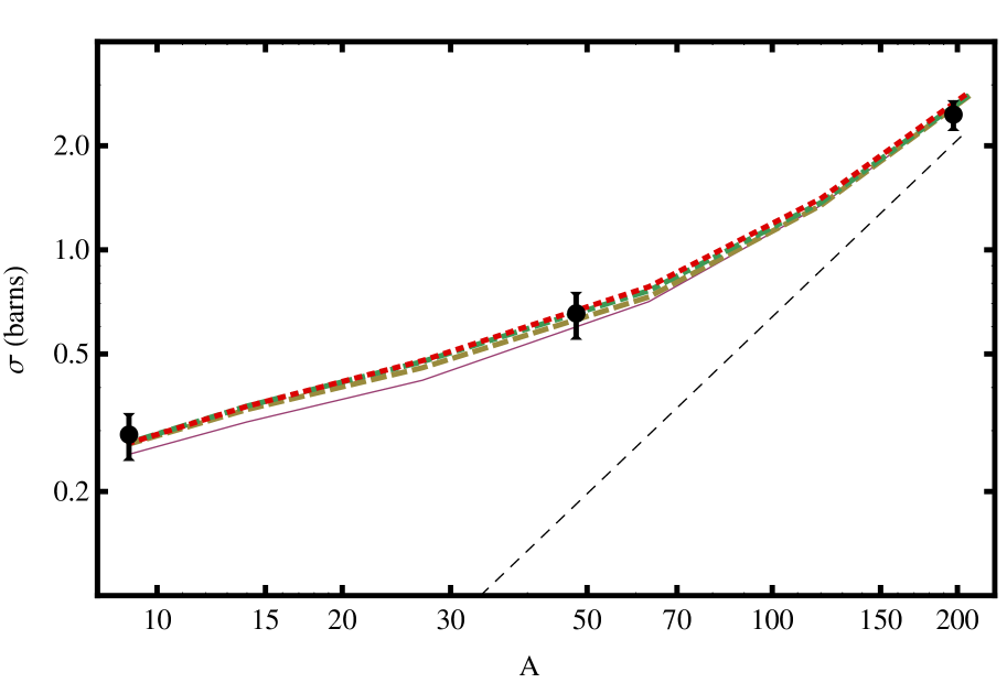
Figure 9: (Color online) Comparison of corrections to scattering data at 41 MeV/nucleon from Anne:1994 . The designations for the lines are the same as in fig. 4, with the Coulomb breakup cross-section in dashed black. Because we did not calculate corrections to the Coulomb cross-section, the corrections appear smaller on this plot at high energies where the Coulomb term is larger.

In this subsection we present the results of applying the Wallace corrections to the total cross-sections described above (eqns. LABEL:Eq:diff, 33, and 34). Our primary results for these calculations are summarized by figs. 8-10.

Figure 8 shows the effect of the first order corrections for scattering at 40 MeV/nucleon. These corrections are generally not negligible for any value of $A$

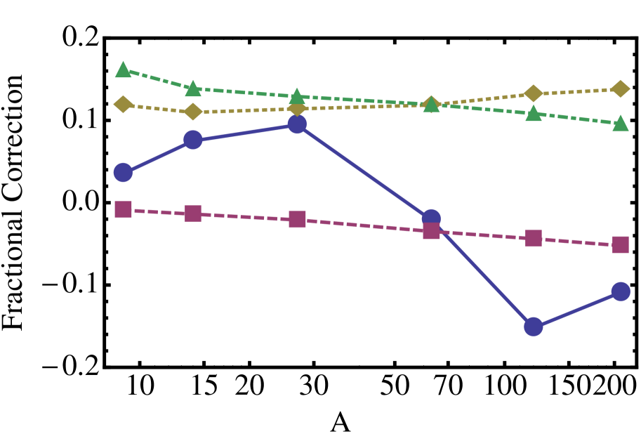
(a) Effect of first-order corrections at beam energy of 40 MeV.

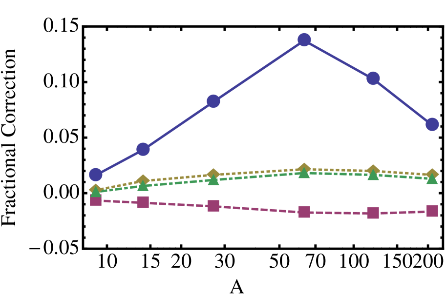
(b) Effect of second-order corrections at beam energy of 40 MeV.

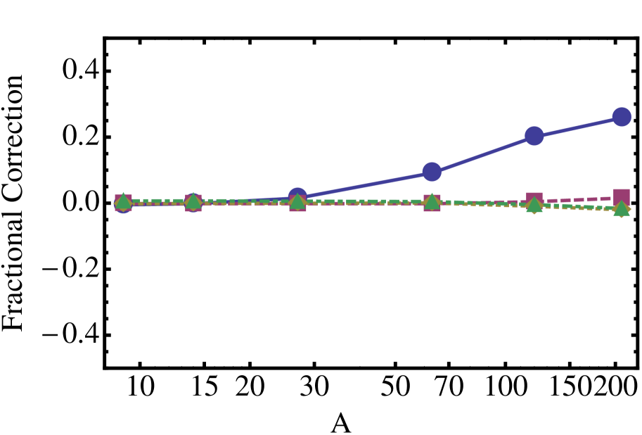
(c) Effect of third-order corrections at beam energy of 40 MeV.

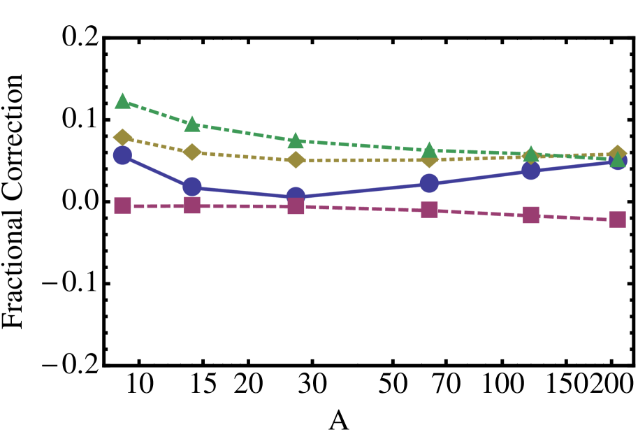
(d) Effect of first-order corrections at a beam energy of 100 MeV/nucleon at beam energy of 40 MeV.

Figure 10: (Color online) Fractional corrections at various orders and beam energies. The designations for the lines are the same as in fig. 8.

Figure 9 compares our results to scattering data collected at 41 MeV/nucleon by Anne et. al. Anne:1994 . The data were collected by detecting the ¹⁰Be core, so the processes that contribute are diffractive scattering, neutron stripping, and Coulomb breakup, which we did not consider. The Coulomb cross-section was taken from Anne:1994 and added to our calculations. Although the corrections have a noticeable effect when compared to the zeroth-order calculations, it is unclear from this data whether the effect is actually significant since the error in the measurements is so large. With more precise experimental measurements the utility of these corrections will become clearer.

Figure 10 gives the fractional correction at each order, which more clearly illustrates the effects of the corrections. The corrections to neutron stripping and total absorption are only significant at first-order, and appear to be independent of $A$. The corrections to diffractive scattering are significant at large values of $A$ all the way through third-order, but are less significant at low values of $A$. We have also performed the same calculations at the higher energy of 100 MeV (see figure 10(d)). As expected, the corrections are smaller at first order (less than 10%), and are less than 1% at higher orders.

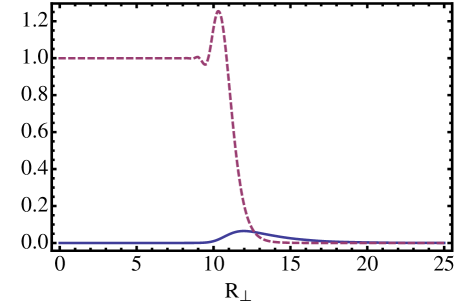
Figure 11: (Color online) The integrand of eq. LABEL:Eq:diff (solid blue) for a ²⁰⁸Pb target, and the second term in the same integrand, which is the elastic scattering for the system (dashed magenta). Both are given as functions of $R_{\perp}$ (see Fig. 7) with all other variables integrated out.

Diffractive scattering is primarily a surface effect, (see Fig. 11) which is why the diffractive corrections have a markedly different behavior as a function of $A$ than the other types of scattering. As $A$ changes, the radius of the target nucleus changes as well. The corrections are larger for surface effects than for volume effects (especially at low energies) because of the derivative operators $\widehat{\beta}_{n}$ that arise. Since diffractive scattering is the only type of scattering studied here that is almost entirely a surface effect, changes in the radius of the target affect it more than the other types of scattering we studied.

V Summary and Discussion

We have calculated corrections to the eikonal approximation to nuclear scattering in an eikonal expansion framework for many different processes. We find that for the case of simple potential scattering it is clear that application of these corrections improves the accuracy of the eikonal approximation at beam energies between 30 and 100 MeV. It is reasonable to expect that the first-order correction would be significant at even higher beam energies.

We also see from application to the interactions of ¹¹Be with nuclei at 40 MeV that these corrections can be as high as 15% for neutron stripping and diffractive scattering. As expected, the corrections decrease as the beam energy increases.

We compare our theory with the data of Anne et al. Anne:1994 and find that the corrections are substantial, although not as large as the experimental uncertainties.

It is interesting to note that the diffractive corrections have a strikingly different behavior from the corrections to stripping and absorption. We attribute this to surface effects that have a stronger influence on diffractive scattering than on the other processes.

The first-order corrected cross-sections do not require much more computational effort to calculate than the zeroth-order calculations. We performed our calculations on an 8 core node of the Hyak scientific computing cluster at the University of Washington, and saw less than a factor of 2 increase in computation time after including the first-order corrections. Even adding in the second- and third-order corrections usually resulted in less than a factor of 2 increase in computation time, although the calculation of the $T$-matrix elements does increase in complexity (eqns. 8-18).

Thus we believe that our proposed framework of using the eikonal approximation as improved by the corrections of Wallace would be a useful way to analyze data produced at FRIB. Future work will focus on specific reactions of experimental interest.

References

- (1) S. J. Wallace, Phys. Rev. Lett. 27, 622 (1971).
- (2) S. J. Wallace, Annals Phys. 78, 190 (1973).
- (3) http://www.nscl.msu.edu/future/nsclwhitepaper2006 “Isotope Science Facility at Michigan State University Upgrade of the NSCL rare isotope research capabilities” MSUCL-1345, Nov. 2006
- (4) P. G. Hansen and J. A. Tostevin, Ann. Rev. Nucl. Part. Sci. 53, 219 (2003).
- (5) A. Gade and T. Glasmacher, Prog. Part. Nucl. Phys. 60, 161 (2008)
- (6) C. A. Bertulani and A. Gade, Phys. Rept. 485, 195 (2010)
- (7) R. J. Glauber, “High Energy Collision Theory”,p. 315 in “Lectures in Theoretical Physics” Ed. by W. E. Brittain and L. G. Dunham, Vol. I, Interscience, New York, 1959 R. J. Glauber, “Theory of high energy hadron-nucleus collisions,” p. 207, In “High-Energy Physics And Nuclear Structure”, ed. by S. Devons, Plenum Press, New York 1970
- (8) G. Bertsch, H. Esbensen and A. Sustich, Phys. Rev. C 42, 758 (1990).
- (9) Y. Ogawa, K. Yabana and Y. Suzuki, Nucl. Phys. A 543, 722 (1992).
- (10) J. S. Al-Khalili, J. A. Tostevin and I. J. Thompson, Phys. Rev. C 54, 1843 (1996).
- (11) T. Aumann, A. Navin, D. P. Balamuth, D. Bazin, B. Blank, B. A. Brown, J. E. Bush and J. A. Caggiano et al., Phys. Rev. Lett. 84, 35 (2000).
- (12) K. Hencken, G. Bertsch and H. Esbensen, Phys. Rev. C 54, 3043 (1996)
- (13) Y. . L. Parfenova, M. V. Zhukov and J. S. Vaagen, Phys. Rev. C 62, 044602 (2000).
- (14) I. Licot, N. Added, N. Carlin, G. M. Crawley, S. Danczyk, J. Finck, D. Hirata and H. Laurent et al., Phys. Rev. C 56, 250 (1997).
- (15) E. Sauvan, F. Carstoiu, N. A. Orr, J. C. Angelique, W. N. Catford, N. M. Clarke, M. Mac Cormick and N. Curtis et al., Phys. Lett. B 491, 1 (2000)
- (16) C. A. Bertulani and A. Gade, Comput. Phys. Commun. 175, 372 (2006)
- (17) H. Esbensen and G. F. Bertsch, Phys. Rev. C 64, 014608 (2001).
- (18) S. J. Wallace, Phys. Rev. D 8, 1846 (1973).
- (19) R. L. Varner, W. J. Thompson, T. L. McAbee, E. J. Ludwig and T. B. Clegg, Phys. Rept. 201, 57 (1991).
- (20) H. de Vries, C. W. de Jager, and C. de Vries, At. Data Nucl. Data Tables 36, 495 (1987).
- (21) R. Anne, et al., Nuc. Phys. A575, 125 (1994).