The validity of quasi steady-state approximations in discrete stochastic simulations

Abstract

In biochemical networks, reactions often occur on disparate timescales and can be characterized as either “fast” or “slow.” The quasi-steady state approximation (QSSA) utilizes timescale separation to project models of biochemical networks onto lower-dimensional slow manifolds. As a result, fast elementary reactions are not modeled explicitly, and their effect is captured by non-elementary reaction rate functions (e.g. Hill functions). The accuracy of the QSSA applied to deterministic systems depends on how well timescales are separated. Recently, it has been proposed to use the non-elementary rate functions obtained via the deterministic QSSA to define propensity functions in stochastic simulations of biochemical networks. In this approach, termed the stochastic QSSA, fast reactions that are part of non-elementary reactions are not simulated, greatly reducing computation time. However, it is unclear when the stochastic QSSA provides an accurate approximation of the original stochastic simulation. We show that, unlike the deterministic QSSA, the validity of the stochastic QSSA does not follow from timescale separation alone, but also depends on the sensitivity of the non-elementary reaction rate functions to changes in the slow species. The stochastic QSSA becomes more accurate when this sensitivity is small. Different types of QSSAs result in non-elementary functions with different sensitivities, and the total QSSA results in less sensitive functions than the standard or the pre-factor QSSA. We prove that, as a result, the stochastic QSSA becomes more accurate when non-elementary reaction functions are obtained using the total QSSA. Our work provides a novel condition for the validity of the QSSA in stochastic simulations of biochemical reaction networks with disparate timescales.

1: Mathematical Biosciences Institute, The Ohio State University, Columbus, OH, 43210;
2: Department of Mathematics, University of Houston, Houston, TX, 77204;
3: Department of Biology and Biochemistry, University of Houston, Houston, TX, 77204;
4: Department of Biochemistry & Cell Biology, Rice University, Houston, TX, 77005;
5: Institute of Biosciences and Bioengineering, Rice University, Houston, TX, 77005;
*: Correspondence: josic@math.uh.edu or matthew.bennett@rice.eduy

Note: This pre-print has been accepted for publication in Biophysical Journal. The final copyedited version of this paper will be available at www.biophyj.org

Introduction

In both prokaryotes and eukaryotes, the absolute number of a given reactant is generally small (1, 2), leading to high intrinsic noise in reactions. The Gillespie algorithm is widely used to simulate such reactions by generating sample trajectories from the chemical master equation (CME) (3). Because the Gillespie algorithm requires the simulation of every reaction, simulation times are dominated by the computation of fast reactions. For example, in an exact stochastic simulation most time is spent on simulating the fast binding and unbinding of transcription factors to their promoter sites, although these reactions are of less interest than transcription which is slower. Thus, the Gillespie algorithm is frequently too inefficient to simulate biochemical networks with reactions spanning multiple timescales (4, 5).

Recently, the slow-scale stochastic simulation algorithm (ssSSA) was introduced to accelerate such simulations  (4, 5) (Fig. 1). The main idea behind the ssSSA is to use the fact that fast species equilibrate quickly. Thus, we can replace fast species by their average values to derive effective propensity functions. These average values can be obtained by applying a quasi-steady-state approximation (QSSA) (6, 7, 8) or quasi-equilibrium approximation (9, 10) to the CME. When using the ssSSA we only need to simulate slow reactions, greatly increasing simulation speed with no significant loss of accuracy (4, 5, 6, 7, 8, 9, 10). However, the utility of the ssSSA is limited by the difficulty of calculating the average values of fast species, which requires knowledge of the joint probability distribution of the CME (4, 5, 6, 7, 10).

To estimate the averages value of the fast species, Rao et al. proposed using the fast species concentration at quasi-equilibrium in the deterministic system (6). In such a stochastic QSSA, the deterministic QSSA is used to approximate the propensity functions obtained via the ssSSA (Fig. 1). Thus, non-elementary macroscopic rate functions (e.g. Hill functions) are used to derive the propensity functions in the same way as elementary rate functions (i.e. those obtained directly from mass action kinetics). Several numerical studies supported the validity of the stochastic QSSA in systems as diverse as Michaelis-Menten enzyme kinetics, bistable switches, and circadian clocks (11, 6, 7, 12). These studies provided evidence that the stochastic QSSA is valid when timescale separation holds (13, 14, 15). Therefore, stochastic simulations of biochemical networks are frequently performed without converting the non-elementary reactions to their elementary forms (16, 17, 18). Moreover, rates of the individual elementary reactions that are jointly modeled using Michaelis-Menten or Hill functions are rarely known, making the use of stochastic QSSA tempting. However, recent studies have demonstrated that, in contrast to the deterministic QSSA, timescale separation does not generally guarantee the accuracy of the stochastic QSSA (13, 14, 15). The stochastic QSSA can often lead to large errors even when timescale separation holds. This raises the question: When is the stochastic QSSA valid?

Here, we investigate the conditions under which the stochastic QSSA is accurate (Fig. 1). We first examine three of the most common reduction schemes: standard QSSA (sQSSA), total QSSA (tQSSA), and pre-factor QSSA (pQSSA). We find that the accuracy of the stochastic QSSA depends on which reduction scheme is used to derive its deterministic counterpart. Specifically, the stochastic tQSSA is more accurate than the stochastic sQSSA or pQSSA (we refer to each stochastic QSSA by the name of its deterministic counterpart, i.e. in the stochastic tQSSA, propensities are derived from the ODEs obtained via the deterministic tQSSA). All three methods relate the fast species concentration in quasi-equilibrium to the slow species concentration. For the tQSSA, this expression is less sensitive to changes in the slow species than either its sQSSA or pQSSA counterparts. We find that for parameters that decrease sensitivity, the stochastic sQSSA and pQSSA also become more accurate. We explain these observations by proving that, as sensitivity decreases, the approximate propensity functions used in the stochastic QSSA converge to the propensity functions obtained using ssSSA (Fig. 1). Furthermore, we use a linear noise approximation (LNA) to show that the accuracy of the stochastic QSSA is determined by both separation of timescales and sensitivity.

In sum, our results indicate that the stochastic QSSA is valid under more restrictive conditions than the deterministic QSSA. Importantly, we identify these conditions, and provide a theoretical foundation for reducing stochastic models of complex biochemical reaction networks with disparate timescales.

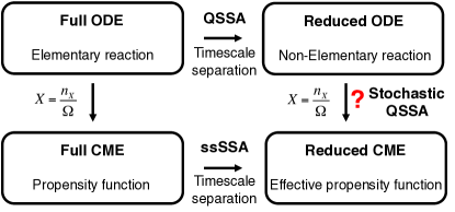
Figure 1: The validity of the stochastic QSSA. Under timescale separation, the full ODE and full CME can be reduced using the deterministic QSSA and ssSSA, respectively. By changing the concentration ($X$) to the number of molecules ($n_{X}$) with the relationship $X=\frac{n_{X}}{\Omega}$ ($\Omega$: the volume of the system), the elementary rate functions in the full ODE can be converted to propensity functions. These are the same as the propensity functions of the full CME, which are derived from collision theory (19). However, the validity of propensity functions derived from non-elementary rate functions (e.g. Hill functions) of the reduced ODE is unclear.

Results

The different types of deterministic QSSA

The term “QSSA” is used to describe a number of related dimensional reduction methods. We first review three common QSSA schemes using the example of a genetic negative feedback model (20, 21). The full model, depicted in Fig. 2A, can be described by the system of ODEs:

$$\dot{M} = \alpha_{M}D_{A}-\beta_{M}M$$ (1)

$$\dot{P} = \alpha_{P}M-\beta_{P}P$$ (2)

$$\dot{F} = \alpha_{F}P-\beta_{F}F-k_{f}FD_{A}+k_{b}D_{R}$$ (3)

$$\dot{D_{R}} = k_{f}FD_{A}-k_{b}D_{R}-\beta_{F}D_{R}$$ (4)

$$\dot{D_{A}} = -k_{f}FD_{A}+k_{b}D_{R}+\beta_{F}D_{R},\$$ (5)

where the transcription of mRNA ($M$) is proportional to the concentration of DNA promoter sites that are free of the repressor protein ($D_{A}$). The mRNA is translated into cytoplasmic protein ($P$). The free repressor protein ($F$) is produced at a rate proportional to the concentration of $P$. The free repressor can bind to a promoter site and change the DNA to its repressed state ($D_{R}$). All species, except for DNA, are subject to degradation ($\beta_{i}$), with the bound and free repressor degrading at the same rate. As can be seen in Eqs. 4 and 5, total DNA concentration ($D_{T}=D_{A}+D_{R}$) is conserved. See Table S1 for the descriptions and values of parameters.

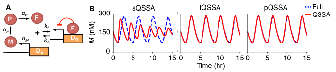
Figure 2: Deterministic QSSA. (A) In the model of a genetic negative feedback loop, the repressor protein ($F$) represses its own transcription by binding to DNA promoter site ($D_{A}$). Reversible binding between $F$ and $D_{A}$ is much faster than other reactions. See Table S1 for parameters. (B) The sQSSA fails to correctly approximate the dynamics of the full system, but both the tQSSA and the pQSSA provide accurate approximations due to complete timescale separation between the variables.

Standard QSSA (sQSSA)

Binding ($k_{f}$) and unbinding ($k_{b}$) between $F$ and $D_{A}$ are much faster than the remaining reactions (Fig. 2A and Table S1). Thus, Eqs. 4 and 5 equilibrate faster than Eqs. 1-3, which leads QSS equations for the fast species ($\dot{D_{R}}=0$ and $\dot{D_{A}}=0$). By solving these QSS equations, we obtain the equilibrium values of fast species ($D_{R}$ and $D_{A}$) in terms of slow species ($F$):

$$D_{R}(F) = \frac{D_{T}F}{F+K_{d}}$$ (6)

$$D_{A}(F) = \frac{D_{T}K_{d}}{F+K_{d}},\$$ (7)

where $K_{d}=(k_{b}+\beta_{F})/k_{f}$. These QSS solutions can be used to close the remaining equations (Eqs. 1-3) giving the reduced system:

$$\dot{M} = \alpha_{M}\frac{D_{T}K_{d}}{F+K_{d}}-\beta_{M}M$$ (8)

$$\dot{P} = \alpha_{P}M-\beta_{P}P$$ (9)

$$\dot{F} = \alpha_{F}P-\beta_{F}\left(F+\frac{D_{T}F}{F+K_{d}}\right).\$$ (10)

This approach is known as the classical or standard QSSA (sQSSA) (22, 23, 24). Previous studies have shown that the sQSSA leads to reductions that correctly predict steady-states, but may not correctly describe the dynamics (25, 26). Indeed, whereas the original system (Eqs. 1-5) relaxes to a limit cycle, the reduced system (Eqs. 8-10) exhibits damped oscillations (Fig. 2B).

Total QSSA (tQSSA)

The inaccuracy of the sQSSA results from treating $F$ as a slow variable, even though it is affected by both slow (production and degradation) and fast (binding and unbinding to DNA) reactions (26). This problem can be solved by introducing the total amount of repressor, $R\equiv F+D_{R}$, instead of $F$. As a result, $\dot{R}$ only depends on slow reactions:

$$\dot{M} = \alpha_{M}D_{A}-\beta_{M}M$$ (11)

$$\dot{P} = \alpha_{P}M-\beta_{P}P$$ (12)

$$\dot{R} = \alpha_{F}P-\beta_{F}R$$ (13)

$$\dot{D}_{R} = k_{f}(R-D_{R})D_{A}-k_{b}D_{R}-\beta_{F}D_{R}$$ (14)

$$\dot{D}_{A} = -k_{f}(R-D_{R})D_{A}+k_{b}D_{R}+\beta_{F}D_{R}.\$$ (15)

By solving the QSS equations for the fast species ($\dot{D_{R}}=0$ and $\dot{D_{A}}=0$), we obtain the equilibrium values of $D_{R}$ and $D_{A}$ in terms of $R$:

$$D_{R}(R) = \frac{1}{2}\left(D_{T}+R+K_{d}-\sqrt{(D_{T}-R-K_{d})^{2}+4D_{T}K_{d}}\right)$$ (16)

$$D_{A}(R) = \frac{1}{2}\left(D_{T}-R-K_{d}+\sqrt{(D_{T}-R-K_{d})^{2}+4D_{T}K_{d}}\right).$$ (17)

Substituting these QSS solutions to close the remaining equations (Eqs. 11-13), we arrive at the reduced system

$$\dot{M} = \alpha_{M}D_{A}(R)-\beta_{M}M$$ (18)

$$\dot{P} = \alpha_{P}M-\beta_{P}P$$ (19)

$$\dot{R} = \alpha_{F}P-\beta_{F}R.\$$ (20)

This approach is known as the total QSSA (tQSSA) (27, 28, 29). Due to the complete timescale separation between variables, the tQSSA leads to a reduced system (Eqs. 18-20) that correctly captures the dynamics of the full system (Fig. 2B). However, unlike the recognizably Michaelis-Menten-like form of sQSS solutions (Eqs. 6 and 7), the corresponding tQSS solutions (Eqs. 16 and 17) are unfamiliar and unintuitive.

Pre-factor QSSA (pQSSA)

The reduced system obtained with the tQSSA can be transformed into a more intuitive form. Expressing Eqs. 18-20 using the original free protein variable, $F$, and using $\dot{R}=\frac{\partial R}{\partial F}\dot{F}$, we obtain:

$$\dot{M} = \alpha_{M}\frac{D_{T}K_{d}}{F+K_{d}}-\beta_{M}M$$ (21)

$$\dot{P} = \alpha_{P}M-\beta_{P}P$$ (22)

$$p(F)\dot{F} = \alpha_{F}P-\beta_{F}\left(F+\frac{D_{T}F}{F+K_{d}}\right),\$$ (23)

where

$$p(F)\equiv\frac{\partial R}{\partial F}=\frac{\partial F}{\partial F}+\frac{\partial D_{R}}{\partial F}=1+\frac{D_{T}K_{d}}{(F+K_{d})^{2}}.$$ (24)

This approach is known as the pre-factor QSSA (pQSSA) (25, 26). We note two important things about Eqs. 21-23. First, the system is identical to that obtained using the sQSSA (Eqs. 8-10), except for the prefactor $p(F)$. Therefore, the two reductions have the same fixed points, but their dynamics are different. The pre-factor is always greater than one, and corrects the inaccuracy in the dynamics that are introduced in the sQSSA (Fig. 2B). Second, because the pQSSA and tQSSA lead to equivalent systems (Eqs. 21-23 and Eqs. 18-20), the resulting dynamics are identical, up to a change of variables. In sum, due to complete timescale separation between variables, reduced ODE models obtained using the tQSSA or the pQSSA approximate the dynamics of the original system more accurately than the sQSSA.

Stochastic QSSA

We have derived the reduced system of a genetic negative feedback model (Eqs. 1-5) using three types of the QSSA. These different reductions result in different propensity functions in the stochastic QSSA. We now investigate how the accuracy of the stochastic QSSA depends on the choice of the reduction.

For discrete stochastic simulations, we need to convert the concentration of a reactant to the absolute number of molecules (Fig. 1). For instance, the concentration of mRNA, $M$, and the number of mRNA molecules, $n_{M}$, are related by $M=n_{M}/\Omega$, where $\Omega$ represents the volume of the system. In this study, we choose $\Omega=1$ for simplicity, so that the numerical values of the concentration and the number of molecules are equal. Using this type of relation, we obtain the propensity functions of the reactions from the corresponding macroscopic rate functions of the full and three reduced ODE models (Tables S2-5). The results of stochastic simulations with these propensity functions are shown in Fig. 3A. Similar to the deterministic simulations (Fig. 2B), the simulations using the stochastic sQSSA exhibit faster oscillations than the full system, and simulations using the stochastic tQSSA correctly predict the dynamics of the full system (Fig. 3A). The deterministic reductions obtained using the tQSSA and the pQSSA are equivalent (Fig. 2B). This suggests that their stochastic counterparts will also behave similarly. However, this is not the case: Simulations using the stochastic pQSSA do not provide an accurate approximation of the full system (Fig. 3A). In particular, the fraction of active DNA, $n_{D_{A}}/n_{D_{T}}$, which determines the transcription rate of mRNA, exhibits large jumps when using the stochastic sQSSA and pQSSA, in contrast to the stochastic tQSSA (Fig. 3A).

This surprising behavior of $n_{D_{A}}/n_{D_{T}}$ when using the stochastic sQSSA and pQSSA is a result of the sensitive dependence of this ratio on the number of free repressor, $n_{F}$:

$$\frac{n_{D_{A}}}{n_{D_{T}}}=\frac{K_{d}\Omega}{n_{F}+K_{d}\Omega}\thickapprox\left\{\begin{array}[]{ll}1&n_{F}=0\\ 0.2&n_{F}=1\\ 0.11&n_{F}=2\\ \vdots&\vdots\end{array},\right.\$$ (25)

which is derived from the non-elementary form of the sQSS solution (Eq. 7). Only a few molecules of transcription factor are needed to strongly repress transcription. Therefore, when the QSS solution (Eq. 7) is used to derive $n_{D_{A}}/n_{D_{T}}$ (Eq. 25) in the case of the stochastic sQSSA or pQSSA, the stochastic simulations become extremely sensitive to fluctuations in $n_{F}$ when $n_{F}$ is small. This is the cause of the large jumps seen in Fig. 3A and the disagreement between the dynamics of the reduced and the original system. The stochastic pQSSA leads to additional errors because the pre-factor defined by Eq. 24 is also sensitive to fluctuations in $n_{F}$ (Fig. 3A).

However, in the stochastic tQSSA, the ratio $n_{D_{A}}/n_{D_{T}}$, which is derived from the tQSS solution (Eq. 17), is less sensitive to changes in the total amount of repressor, $n_{R}$:

$$\frac{n_{D_{A}}}{n_{D_{T}}} = \frac{1}{2n_{D_{T}}}\left(n_{D_{T}}-n_{R}-K_{d}\Omega+\sqrt{\left(n_{D_{T}}-n_{R}-K_{d}\Omega\right)^{2}+4K_{d}\Omega n_{D_{T}}}\right)$$ (30)

$$\thickapprox \left\{\begin{array}[]{ll}1&n_{R}=0\\ 0.993939&n_{R}=1\\ 0.98789&n_{R}=2\\ \vdots&\vdots\end{array}\right.\$$

As a result, the ratio $n_{D_{A}}/n_{D_{T}}$ does not exhibit large jumps, and the dynamics of the original system are approximated accurately when using the stochastic tQSSA (Fig. 3A).

The sensitivity of the ratio $n_{D_{A}}/n_{D_{T}}$ to changes in $n_{F}$ depends on system parameters. We expect that when this sensitivity is small, the stochastic sQSSA or pQSSA become more accurate. One way to reduce such sensitivity is to increase $K_{d}$ in Eq. 25. As $K_{d}$ increases, the deterministic system ceases to oscillate and asymptotically approaches a fixed point, so that we can measure the coefficient of variation (CV) of $n_{M}$ at equilibrium to describe the variability in the system. As shown in Fig. 3B, as $K_{d}$ increases and the sensitivity of Eq. 25 decreases, the stochastic sQSSA and pQSSA become more accurate. Furthermore, the stochastic tQSSA is accurate at all values of $K_{d}$ due to the low sensitivity of Eq. 30.

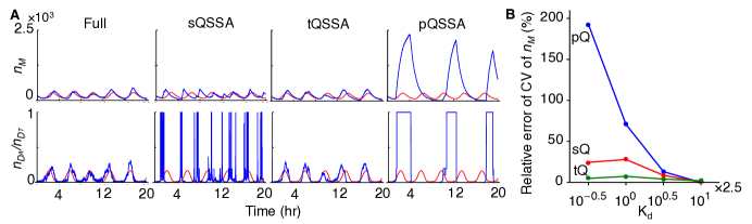
Figure 3: Stochastic QSSA. (A) Whereas the deterministic pQSSA and tQSSA are equivalent (Fig. 2B), simulation results of the stochastic pQSSA and tQSSA do not agree. In particular, the amount of active DNA, described by Eqs. 25 and 30, exhibits large jumps when using the sQSSA and the pQSSA, but not the tQSSA. Results of the deterministic simulation of the full system are shown in red, while results of the stochastic simulations are shown in blue. (B) As $K_{d}$ increases, the sensitivity of the QSS solution (Eq. 25) decreases, which results in more accurate simulations of the stochastic QSSA. The coefficient of variation (CV) of mRNA $(n_{M})$ at its steady state is estimated with 25,000 independent simulations for each system. Each simulation is run until 20 hr of reaction time to ensure the system in the stationary state.

The accuracy of the stochastic QSSA depends on the sensitivity of the QSS solution

We next provide a more complete analysis of the relationship between the sensitivity of the QSS solution and the accuracy of the stochastic QSSA. In our model, the reversible binding between free repressor protein and DNA,

$$F+D_{A}{\longleftrightarrow}D_{R},$$ (31)

is much faster than other reactions. The amount of active DNA is governed by this fast reaction and determines the dynamics of the slow process, specifically the transcription of mRNA with propensity function $\alpha_{M}n_{D_{A}}$. Previous studies have shown that, assuming timescale separation, this propensity function can be approximated by an effective propensity function, $\alpha_{M}\left<n_{D_{A}}\right>$ (4, 5, 10). This approach is known as the ssSSA (Fig. 1). Here, the average, $\left<\cdot\right>,$ is defined by

$$\left<x\right>\equiv\sum_{x=0}^{\infty}xP(x|\mathbb{S}),$$ (32)

where $P(x|\mathbb{S})$ is the stationary probability distribution of $x$ given a fixed state, $\mathbb{S},$ of slow species. That is, we compute the average of the fast species in quasi-equlibrium. Hence, $\left<n_{D_{A}}\right>$ is the mean of the steady-state distribution of active DNA evolving only through fast reactions, with slow species “frozen” in time. The main idea behind the ssSSA is that $n_{D_{A}}$ quickly relaxes to $\left<n_{D_{A}}\right>$, so that over slow timescales $n_{D_{A}}$ can be replaced with $\left<n_{D_{A}}\right>$ (Fig. 1) (4, 5, 10). However, $\left<n_{D_{A}}\right>$ is usually unknown, so the stochastic QSSA approximates $\left<n_{D_{A}}\right>$ with a QSS solution. One can estimate the error in using either the sQSS solution $n_{D_{A}}(n_{F})$ (Eq. 25) or the tQSS solution $n_{D_{A}}(n_{R})$ (Eq. 30) to approximate $\left<n_{D_{A}}\right>$ by equating moments (12) (see supplementary information for details). For the stochastic sQSSA and pQSSA this leads to

$$\left<n_{D_{A}}\right>\approx n_{D_{A}}(\left<n_{F}\right>)+\frac{Var(n_{D_{A}})}{n_{D_{A}}(\left<n_{F}\right>)}\frac{dn_{D_{A}}(\left<n_{F}\right>)}{d\left<n_{F}\right>},$$ (33)

and for the stochastic tQSSA we arrive at

$$\left<n_{D_{A}}\right>\approx n_{D_{A}}(n_{R})+\frac{Var(n_{D_{A}})}{n_{D_{A}}(n_{R})}\frac{dn_{D_{A}}(n_{R})}{dn_{R}}.$$ (34)

Here, $n_{D_{A}}(\left<n_{F}\right>)$ in Eq. 33 agrees with the expression for $n_{D_{A}}(n_{F})$ derived from the sQSS solution (Eq. 25) because $\left<n_{F}\right>$ approximates $n_{F}$ under slow timescale. The errors of both the sQSS and tQSS solutions above depend on the Fano factor of the fast species, $\frac{Var(n_{D_{A}})}{n_{D_{A}}}$, because the QSS solutions agree with $\left<n_{D_{A}}\right>$ under the moment closure assumption (see supplementary information for details). That is, the error in the stochastic QSSA arises mainly from ignoring the variance of fast variables, which will vanish along with random fluctuations in the limit of large system size. Interestingly, the magnitude of the error depends on the sensitivity of the QSS solution. In particular, $\frac{dn_{D_{A}}}{dn_{R}}$, the sensitivity of the tQSS solution (Eq. 30), is small because $|\frac{dn_{D_{A}}}{dn_{R}}|=|\frac{dn_{D_{R}}}{dn_{R}}|<1$ regardless of parameter choice. This explains the accuracy of the stochastic tQSSA (Fig. 3). However, the sensitivity of the sQSS solution ($\frac{dn_{D_{A}}(\left<n_{F}\right>)}{d\left<n_{F}\right>}$) can be large (Eq. 25). Eq. 33 implies that the accuracy of the stochastic sQSSA and pQSSA deteriorates as $\frac{dn_{D_{A}}(\left<n_{F}\right>)}{d\left<n_{F}\right>}$ increases, which explains our previous simulation results (Fig. 3). From Eqs. 33 and 34, we can also compare the errors of the two approximations obtained with the sQSSA and the tQSSA:

$$\frac{\left<n_{D_{A}}\right>-n_{D_{A}}(\left<n_{F}\right>)}{\left<n_{D_{A}}\right>-n_{D_{A}}(n_{R})}\approx\frac{dn_{D_{A}}(\left<n_{F}\right>)}{d\left<n_{F}\right>}\big{/}\frac{dn_{D_{A}}(n_{R})}{dn_{R}}=\frac{dn_{R}}{d\left<n_{F}\right>}=1+\frac{d\left<n_{D_{r}}\right>}{d\left<n_{F}\right>}>1.$$ (35)

This inequality follows from the observation that $\left<n_{D_{R}}\right>$ increases monotonically with $\left<n_{F}\right>$. Eq. 31 indicates that the tQSSA provides a better estimate of $\left<n_{D_{A}}\right>$ than the sQSSA or the pQSSA. More generally, the tQSS solution has lower sensitivity than sQSS or pQSS solutions if the components of the total variable used in the tQSSA have a positive, monotonic relationship with the variable used in the sQSSA or the pQSSA. That is, let us assume that $T=T_{1}+T_{2}+...+T_{n}$ is the total variable used in the tQSSA (e.g. $R$) and $T_{1}$ is the slow variable used for the sQSSA and the pQSSA (e.g. $F$). If $\frac{dT_{i}}{dT_{1}}>0$ for all $i=2,...,n$, then the tQSS solution always has lower sensitivity than the sQSS solution or the pQSS solution. Widely used QSS solutions, such as Hill-functions, satisfy this condition.

In summary, the non-elementary form of the QSS solutions derived using the sQSSA and the tQSSA provide estimates of the first moment of the fast species under a moment closure assumption, but with different choices of coordinates (Fig. 1). The error introduced by truncating higher moments depends on the sensitivity of the QSS solutions in both cases. These results are generalized to any system in which reversible binding reactions are faster than other reactions. The proof of the following theorem can be found in the supplementary information.

Theorem. Assume that a biochemical reaction network includes a reversible binding reaction with a dissociation constant $K_{d}=k_{b}/k_{f}$,

$$S+F{\longleftrightarrow}C.$$ (36)

that is faster than the other reactions in the system. Let $T\equiv S+C$ and $U\equiv F+C$. If $Var(n_{C})\ll n_{T}n_{U}$, then $\left<n_{C}\right>$ and $\left<n_{F}\right>$ satisfy:

$$\left<n_{C}\right> \approx n_{C}(n_{T})+\frac{Var(n_{C})}{n_{F}(n_{T})}\frac{dn_{C}(n_{T})}{dn_{T}}$$ (37)

$$\left<n_{F}\right> \approx n_{F}(n_{T})+\frac{Var(n_{F})}{n_{F}(n_{T})}\frac{dn_{F}(n_{T})}{dn_{T}},\$$ (38)

where $n_{C}(n_{T})$ is the solution of the tQSS equation, $n_{C}^{2}-(n_{U}+n_{T}+K_{d}\Omega)n_{C}+n_{U}n_{T}=0$, and $n_{F}(n_{T})=n_{U}-n_{C}(n_{T})$. Similarly,

$$\left<n_{C}\right> \approx n_{C}(\left<n_{S}\right>)+\frac{Var(n_{C})}{n_{F}(\left<n_{S}\right>)}\frac{dn_{C}(\left<n_{S}\right>)}{d\left<n_{S}\right>}$$ (39)

$$\left<n_{F}\right> \approx n_{F}(\left<n_{S}\right>)+\frac{Var(n_{F})}{n_{F}(\left<n_{S}\right>)}\frac{dn_{F}(\left<n_{S}\right>)}{d\left<n_{S}\right>},\$$ (40)

where $n_{C}(\left<n_{S}\right>)$ is the solution of the sQSS equation, $(\left<n_{S}\right>+K_{d}\Omega)n_{F}+n_{U}\left<n_{S}\right>=0$, and $n_{F}(\left<n_{S}\right>)=n_{U}-n_{C}(\left<n_{S}\right>)$.

Michaelis-Menten enzyme kinetics

We first apply our theorem to Michaelis-Menten enzyme kinetics (22, 30) under the assumption that the product of the reaction can revert back to substrate. This example was recently used to explore the accuracy of the stochastic sQSSA (14). The deterministic model is described by:

$$\dot{S} = -k_{f}SE+k_{b}C+k_{s}P$$ (41)

$$\dot{C} = k_{f}SE-k_{b}C-k_{p}C$$ (42)

$$\dot{P} = k_{p}C-k_{s}P,\$$ (43)

where the total enzyme concentration, $E_{T}\equiv C+E$, is constant. In this system, the free enzyme ($E$) reversibly binds substrate ($S$) to form the complex ($C$). The complex irreversibly dissociates into product ($P$) and free enzyme. The products can be converted back to substrate, and hence the substrate concentration is not equal to zero in steady state. We assume that binding ($k_{f}$) and unbinding ($k_{b}$) between $S$ and $E$ are much faster than the other reactions (see Table S6 for the details of parameters). Then, using conservation, $S_{T}\equiv S+C+P$ and solving the QSS equation ($\dot{C}=0$), we obtain the sQSSA system,

$$\dot{S}=-k_{p}C(S)+k_{s}(S_{T}-S-C(S)),$$ (44)

where $C(S)=\frac{E_{T}S}{K_{m}+S}$ and $K_{m}=(k_{b}+k_{p})/k_{f}$. Next, if we define $T\equiv S+C$, we obtain the tQSSA system,

$$\dot{T}=-k_{p}C(T)+k_{s}(S_{T}-T),$$ (45)

where $C(T)=\frac{E_{T}+K_{m}+T-\sqrt{(E_{T}+K_{m}+T)^{2}-4E_{T}T}}{2}$. In the stochastic QSSA, by chaining the concentration to the number of molecules in these QSS solutions (Eqs 44 and 45), we approximate the average of fast species at quasi-equilibrium ($\left<n_{C}\right>$). Then, we can derive the relative errors of these approximations according to Eqs. 37 and 39:

$$\displaystyle\frac{\left<n_{C}\right>-n_{C}(n_{T})}{\left<n_{C}\right>} \approx \frac{1}{\left<n_{C}\right>}\frac{Var(n_{C})}{n_{E}(n_{T})}\frac{dn_{C}(n_{T})}{dn_{T}},$$ (46)

$$\displaystyle\frac{\left<n_{C}\right>-n_{C}(\left<n_{S}\right>)}{\left<n_{C}\right>} \approx \frac{1}{\left<n_{C}\right>}\frac{Var(n_{C})}{n_{E}(\left<n_{S}\right>)}\frac{dn_{C}(\left<n_{S}\right>)}{d\left<n_{S}\right>}.$$ (47)

Similar to Eq. 35, $\frac{dn_{C}/dn_{S}}{dn_{C}/dn_{T}}>1$ regardless of parameter choice. For illustration we select two sets of parameters: for the first $\frac{dn_{C}/dn_{S}}{dn_{C}/dn_{T}}\approx 1$ (Fig. 4A), and for the second $\frac{dn_{C}/dn_{S}}{dn_{C}/dn_{T}}>1$ (Fig. 4B). As expected from Eqs. 46-47, with the first choice of parameters, tQSS and sQSS solutions give comparable results in estimating $\left<n_{C}\right>$ (Fig. 4C). With the second parameter set, the sQSS solution leads to much larger errors than the tQSS solution (Fig. 4D). Furthermore, Eq. 46 and 47 predicts that the error ratio depends on the ratio of sensitivities of the sQSS and tQSS solutions ($\frac{dn_{C}/dn_{S}}{dn_{C}/dn_{T}}$). This prediction is supported by our simulations (Fig. 4E and F). Along with successful estimation of $\left<n_{C}\right>$ when parameters are chosen so that $\frac{dn_{C}/dn_{S}}{dn_{C}/dn_{T}}\approx 1$, the stochastic simulations of slow variables using both the sQSSA (Eq. 44) and the tQSSA (Eq. 45) become accurate (Fig. 4G). However, for the parameters such that $\frac{dn_{C}/dn_{S}}{dn_{C}/dn_{T}}\gg 1$, the stochastic sQSSA results in much larger error than the stochastic tQSSA (Fig. 4H).

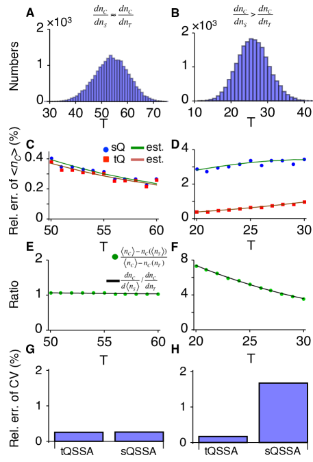
Figure 4: The stochastic QSSA of enzyme kinetics. (A, B) The distribution of $T$ of $20,000$ independent stochastic simulations of the full model (Eqs. 41 - 43) for parameter sets having similar sensitivities (A) and different sensitivities (B) of sQSS and tQSS solutions (see Table S6 for parameters). Each simulation is run for 15000s of reaction time to ensure the system is in equilibrium. (C, D) The errors of QSS solutions used to approximate $\left<n_{C}\right>$ for a given $T$. Blue circles and red squares indicate relative errors of the tQSS solution (left side of Eq. 46) and the sQSS solution (left side of Eq. 47), respectively. Orange and green line indicate our estimates of the relative errors (right sides of Eqs. 46 and 47). (E, F) The ratio between the errors with sQSS and tQSS solutions in Fig. 4C and D matches the ratio between the sensitivities of the sQSS and tQSS solutions. (G, H) Relative errors of the CV of the slow species when the stochastic sQSSA (Eq. 44) and tQSSA (Eq. 45) are used.

Genetic negative feedback loop with protein dimerization

Next, we consider a more complex system that includes multiple fast reversible binding reactions. We adopt a model of the $\lambda$ repressor protein cI of phage $\lambda$ in E. coli (31, 32), in which a dimeric protein represses its own transcription. The slow reactions in the model consist of transcription, translation, and degradation:

$$D_{A} \xrightarrow{\alpha_{M}} D_{A}+M$$ (48)

$$M \xrightarrow{\alpha_{P}} M+P$$ (49)

$$M \xrightarrow{\beta_{M}} \phi$$ (50)

$$P \xrightarrow{\beta_{P}} \phi,\$$ (51)

where $D_{A}$ is free DNA, $M$ is mRNA, and $P$ is monomeric protein. See Table S7 for the details of parameters. The fast reactions of the model are the dimerization of monomer and the binding of the dimer to the DNA,

$$P+P \xleftrightarrow[\text{$k_{b1}$}]{\text{$k_{f1}$}} P_{2}$$ (52)

$$P_{A}+D_{A} \xleftrightarrow[\text{$k_{b2}$}]{\text{$k_{f2}$}} D_{R},\$$ (53)

where $P_{2}$ is dimeric protein and $D_{R}$ is DNA bound to the dimer. By applying the QSSA to these two fast reactions, we obtain the sQSS solutions for $P_{2}$ and $D_{A}$ in terms of $P$: $P_{2}(P)=P^{2}/K_{1}$ and $D_{A}(P)=\frac{K_{2}}{K_{2}+P_{2}(P)}$, where $K_{1}=k_{b1}/k_{f1}$ and $K_{2}=k_{b2}/k_{f2}$. If we define $T\equiv P+2P_{2}+D_{R}$ and assume $D_{R}\ll T$, we obtain the tQSS solutions for $P_{2}$ and $D_{A}$ in terms of $T$: $P_{2}(T)\approx\frac{K_{1}+4T-\sqrt{K^{2}_{1}+8K_{1}T}}{2}$ and $D_{A}(T)=\frac{K_{2}}{K_{2}+P_{2}(T)}$. We use these QSS solutions to derive the propensity functions for the stochastic sQSSA and tQSSA. When the sensitivities of the sQSS solutions are much larger than those of the tQSS solutions (Fig. 5A), the stochastic sQSSA produces much larger errors in the average value of the fast variables, $P_{2}$ and $D_{A}$ than the stochastic tQSSA (Fig. 5C and E). As a result, the stochastic sQSSA results in a larger error in the CV of the slow variable, $n_{M}$, than the stochastic tQSSA (Fig. 5 G). When the sensitivities of the sQSS solutions are reduced by changing parameters (Fig. 5B), the stochastic sQSSA more accurately predicts the average value of fast variables, $P_{2}$ and $D_{A}$ (Fig. 5D and F). Hence, the relative error in the CV of the slow variable, $n_{M}$, decreases (Fig. 5H).

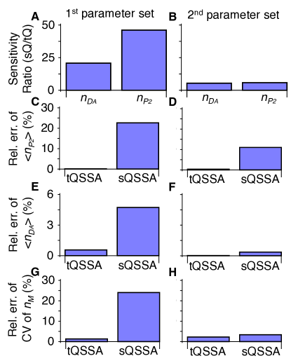
Figure 5: Genetic negative feedback loop with protein dimerization. (A, B) $\frac{dn_{D_{A}}/dn_{P}}{dn_{D_{A}}/dn_{T}}$ and $\frac{dn_{P_{2}}/dn_{P}}{dn_{P_{2}}/dn_{T}}$, ratios between the sensitivities of sQSS and tQSS solutions for $n_{D_{A}}$ and $n_{P_{2}}$ at equilibrium of two parameter sets (see Table S7 for parameters). (C-F) Relative errors of the averages of fast species simulated using the stochastic QSSA. Here, $\left<n_{D}\right>$ and $\left<n_{P_{2}}\right>$ are the average of $n_{D}$ and $n_{F}$ at equilibrium. (G, H) Relative errors of CV of a slow specie, $n_{M},$ at equilibrium. The results were obtained from 50,000 independent simulations. Each simulation is run until 5000s for the first parameter set and 15000s for the second parameter set of reaction time to ensure the system in the stationary state.

Linear noise approximation under slow timescales

We have shown that the accuracy of the stochastic QSSA depends on both the sensitivity of the QSS solution and the variance of fast species (Eqs. 37-40). However, the variance of fast species is usually unknown. Here, we derive the error in the variance of slow species simulated with the stochastic QSSA without using the variance of fast species. For this, we use a LNA that allows the estimation of the variance of variables in a mono-stable system when the number of molecules is not too small (13, 15, 14, 33). Thus, with LNA, we can estimate the variance of slow species in the stochastic QSSA and compare with the original system.

Consider a two dimensional deterministic system that consists of a slow species, $S,$ and a fast species, $F$,

$$\begin{array}[]{l}\displaystyle\dot{S}=u(S,F),\\ \displaystyle\dot{F}=v(S,F).\end{array}$$ (54)

If the system is monostable, the corresponding LNA is given by

$$\dot{\eta_{S}} = u_{S}\eta_{S}+u_{F}\eta_{F}+\frac{1}{\sqrt{\Omega}}S_{S}\sqrt{A}\vec{\Gamma}(t)$$ (55)

$$\dot{\eta_{F}} = v_{F}\eta_{S}+v_{F}\eta_{F}+\frac{1}{\sqrt{\Omega}}S_{F}\sqrt{A}\vec{\Gamma}(t),\$$ (56)

whose solutions, $\eta_{S}$ and $\eta_{F}$ provide approximations for the size of fluctuation of $S$ and $F$ from their steady state. $S_{S}$ and $S_{F}$ are stoichiometry matrices involving the variable $S$ and $F$, respectively; $A$ is a diagonal matrix whose entries are the elements of macroscopic rate functions; and $u_{S},u_{F},v_{S}$, and $v_{F}$ are components of the Jacobian at the steady state. Furthermore, $\vec{\Gamma}(t)$ is a vector of Gaussian noise whose elements, $\Gamma_{i}(t)$ for $i\in\left\{S,F\right\}$, satisfying $\left<\Gamma_{i}(t)\right>=0,$ and $\left<\Gamma_{i}(t)\Gamma_{j}(t^{\prime})\right>=\delta_{ij}\delta(t-t^{\prime}),$ where $\delta_{ij}$ and $\delta(t)$ are the Kronecker and Dirac $\delta$-functions, respectively. Because the solutions of the LNA ($\eta_{S}$ and $\eta_{F}$) are multivariate Gaussian probability distributions, we can approximate the variance of $S$ and $F$, which is difficult to obtain from the original full CME (13, 15, 14, 33). Recently, Thomas et al. (15) showed that when timescale separation holds, the effective stochastic description of intrinsic noise in the slow species can be described by the slow-scale LNA (ssLNA):

$$\dot{\eta_{S}}=(u_{S}-u_{F}v^{-1}_{F}v_{S})\eta_{S}+\frac{1}{\sqrt{\Omega}}(S_{S}-u_{F}v^{-1}_{F}S_{F})\sqrt{A}\vec{\Gamma}(t).$$ (57)

From this ssLNA, the variance of slow species ($\sigma_{S}$) can be derived by solving the Lyapunov equation (33),

$$\sigma_{S}=\frac{S^{\prime}AS^{\prime-1}}{2J\Omega},$$ (58)

where $S^{\prime}=S_{S}-u_{F}v^{-1}_{F}S_{F}$ and $J=u_{S}-u_{F}v^{-1}_{F}v_{S}$.

Thomas et al. (15) also derived the LNA corresponding to the reduced deterministic system with the QSSA:

$$\dot{\eta_{S}}=(u_{S}-u_{F}v^{-1}_{F}v_{F})\eta_{S}+\frac{1}{\sqrt{\Omega}}S_{S}\sqrt{A}\vec{\Gamma}(t).$$ (59)

This is the LNA of the reduced stochastic model obtained via the stochastic QSSA. The diffusion term of this LNA does not have $u_{F}v^{-1}_{F}S_{F}$ in contrast to the ssLNA. Thus, the LNA corresponding to the stochastic QSSA (Eq. 59) predicts the variance of slow species ($\sigma_{S}$), which is different from Eq. 58 of the ssLNA:

$$\sigma_{S}=\frac{S_{S}AS_{S}^{-1}}{2J\Omega},$$ (60)

where $J=u_{S}-u_{F}v^{-1}_{F}v_{S}$. Because $u_{F}v^{-1}_{F}S_{F}$ represents the contribution of the fast species to the variation of the slow species (15), the difference between Eq. 58 and Eq. 60 indicates that the stochastic QSSA does not include the contribution of fast species to the variation of slow species. This is consistent with our moment analysis, which shows that the error of the stochastic QSSA stems from ignoring the variance of the fast species. Furthermore, $u_{F}v^{-1}_{F}$, which determines the error in $\sigma_{S}$ (Eq. 60) simulated with the stochastic QSSA, can be directly calculated from the Jacobian of the deterministic system. Thus, by calculating $u_{F}v^{-1}_{F}$ of the deterministic system used in the tQSSA or sQSSA, we can estimate the accuracy of $\sigma_{S}$ simulated with the stochastic tQSSA or sQSSA.

If we define $T\equiv S+F$, then from Eq. 54, it follows that

$$\dot{T} = u(S,F)+v(S,F)\equiv\overline{u}(T,F)$$ (61)

$$\dot{F} = v(S,F)\equiv\overline{v}(T,F).\$$ (62)

Then, the error in the diffusion term of the LNA corresponding to the stochastic tQSSA will be $\overline{u}_{F}\overline{v}^{-1}_{F}$. Implicit differentiation of the tQSS equation, $\overline{v}(T,F)=0$, gives $\frac{dF(T)}{dT}=-\frac{\overline{v}_{T}}{\overline{v}_{F}}$. From this, we can find the error in the diffusion term of the LNA corresponding to the stochastic tQSSA.

$$\frac{\overline{u}_{F}}{\overline{v}_{F}}=-\frac{\overline{u}_{F}}{\overline{v}_{T}}\frac{dF(T)}{dT}.$$ (63)

Note that the error depends on the sensitivity of the tQSS solution, $\frac{dF(T)}{dT}$. In the example of Michaelis-Menten enzyme kinetics (Eqs. 41-42), the right side of Eq. 63 becomes $\frac{k_{p}}{k_{f}E}\frac{dC(T)}{dT}$. This will be small because $\frac{dC(T)}{dT}\leq 1$ and $\frac{k_{p}}{k_{f}E}\ll 1$ due to timescale separation. This indicates that the stochastic tQSSA will accurately approximate the variance of slow species as long as timescale separation holds (Fig. 4).

In a similar way, we can derive the error of diffusion term in the LNA corresponding to the stochastic sQSSA (see supplementary information for details):

$$-\frac{u_{F}+v_{F}}{v_{S}}\frac{dF(S)}{dS}.$$ (64)

The error in the diffusion term of the stochastic sQSSA also depends on the the sensitivity of the sQSS solution,$\frac{dF(S)}{dS}$. In the example of Eqs. 41-42, Eq. 64 becomes $\frac{k_{p}+k_{s}}{k_{f}E}\frac{dC(S)}{dS}$. Due to timescale separation,$\frac{k_{p}+k_{s}}{k_{f}E_{T}}\ll 1$. However, in contrast to $\frac{dC(T)}{dT}\leq 1$, $\frac{dC(S)}{dS}$ can be very large depending on the parameter choice. Thus, even with timescale separation, the stochastic sQSSA cannot provide an accurate approximation for the variance of slow species if $\frac{dC(S)}{dS}$ is large. Furthermore, from Eqs. 63 and 64, we can show that the ratio between these errors depends on $\frac{dF(S)/dS}{dF(T)/dT}$ similar to Eq. 35 (see supplementary information for details). In summary, LNA analysis shows that the sensitivity of the QSS solution and timescale separation determine the error in the variance of slow species simulated with the stochastic QSSA.

Discussion

Various deterministic QSSAs have been used to reduce ODE models of biochemical networks (22, 30, 23, 25, 24, 26, 27, 28, 29). Recently, the macroscopic reaction rates obtained using deterministic QSSAs have been used to derive approximate propensity functions for discrete stochastic simulations of slowly changing species (Fig. 1). Since this stochastic QSSA does not simulate rapidly fluctuating species, it greatly increases computation speed. The implicit assumption underlying this approach is that the stochastic QSSA is valid whenever its deterministic counterpart is valid, i.e. whenever timescale separation holds (11, 6, 20, 17, 12). If this were true, both the stochastic pQSSA and tQSSA would be equally accurate since their deterministic counterparts are dynamically equivalent (Fig. 2). However, our simulations show that this is not always true and the stochastic tQSSA is more accurate than the stochastic pQSSA (Fig. 3A).

We find that the accuracy of the stochastic QSSA is determined not only by timescale separation, but also the sensitivity of the QSS solution, which relates the fast species and the slow species at quasi-equilibrium (Fig. 3B). Specifically, our analysis of the moment equations shows that the sensitivity of QSS solutions determines how accurately the propensity functions obtained with the stochastic QSSA approximate the effective propensity functions obtained via the ssSSA (Fig. 4). This indicates that the propensity functions obtained from non-elementary reaction rate functions (e.g. Hill function) are accurate only when their sensitivity is low, which provides a novel condition for the validity of the stochastic QSSA. The error in the stochastic QSSA also depends on the variance of fast species, which is usually unknown. Therefore, low sensitivity does not guarantee the accuracy of the stochastic QSSA if the variance of fast species is too large. To address this problem, we also derived the error for the stochastic QSSA using LNA and noted that it does not depend on the variance of fast species. We showed that for a mono-stable two dimensional system, the low sensitivity of the QSS solution is a sufficient condition for the accuracy of stochastic QSSA as long as timescale separation holds. It will be interesting to test whether the low sensitivity of the QSS solution is a sufficient condition in more complex systems.

Whereas the stochastic QSSA uses the QSS solutions to approximate the average values of fast species (4, 6, 7, 8, 10), other methods (e.g. recursion relations) have been proposed to estimate the averages of fast species (9, 10, 14). These other methods could be used as alternatives when the stochastic QSSA is inaccurate (i.e. if the sensitivity of QSS solution is large). Finally, while the stochastic tQSSA is more accurate than the sQSSA or pQSSA, it is often difficult to find a closed form of the tQSS solution, and it needs to be calculated numerically (28, 29). It will be important to understand how numerical calculation of the tQSS solutions affects computation time when using the stochastic tQSSA.

References

- Ghaemmaghami et al. (2003) Ghaemmaghami, S., W.-K. Huh, K. Bower, R. W. Howson, A. Belle, N. Dephoure, E. K. O’Shea, and J. S. Weissman, 2003. Global analysis of protein expression in yeast. Nature 425:737–41.
- Ishihama et al. (2008) Ishihama, Y., T. Schmidt, J. Rappsilber, M. Mann, F. U. Hartl, M. J. Kerner, and D. Frishman, 2008. Protein abundance profiling of the Escherichia coli cytosol. BMC genomics 9:102.
- Gillespie (1977) Gillespie, D. T., 1977. Exact Stochastic Simulation of Coupled Chemical-Reactions. J. Chem. Phys. 81:2340–2361.
- Gillespie (2007) Gillespie, D. T., 2007. Stochastic simulation of chemical kinetics. Ann. Rev. Phys. Chem. 58:35–55.
- Cai and Wang (2007) Cai, X., and X. Wang, 2007. Stochastic modeling and simulation of gene networks-a review of the state-of-the-art research on stochastic simulations. IEEE Signal Process. Mag. 24:27–36.
- Rao and Arkin (2003) Rao, C. V., and A. P. Arkin, 2003. Stochastic chemical kinetics and the quasi-steady-state assumption: Application to the Gillespie algorithm. J. Chem. Phys. 118:4999–5010.
- Barik et al. (2008) Barik, D., M. R. Paul, W. T. Baumann, Y. Cao, and J. J. Tyson, 2008. Stochastic simulation of enzyme-catalyzed reactions with disparate timescales. Biophys. J. 95:3563–3574.
- MacNamara et al. (2008) MacNamara, S., A. M. Bersani, K. Burrage, and R. B. Sidje, 2008. Stochastic chemical kinetics and the total quasi-steady-state assumption: Application to the stochastic simulation algorithm and chemical master equation. J. Chem. Phys. 129.
- Goutsias (2005) Goutsias, J., 2005. Quasiequilibrium approximation of fast reaction kinetics in stochastic biochemical systems. J. Chem. Phys. 122.
- Cao et al. (2005) Cao, Y., D. T. Gillespie, and L. R. Petzold, 2005. The slow-scale stochastic simulation algorithm. J. Chem. Phys. 122.
- Gonze et al. (2002) Gonze, D., J. Halloy, and A. Goldbeter, 2002. Deterministic versus stochastic models for circadian rhythms. J. Biol. Phys. 28:637–653.
- Sanft et al. (2011) Sanft, K. R., D. T. Gillespie, and L. R. Petzold, 2011. Legitimacy of the stochastic Michaelis-Menten approximation. IET Syst. Biol. 5:58–69.
- Thomas et al. (2011) Thomas, P., A. V. Straube, and R. Grima, 2011. Communication: limitations of the stochastic quasi-steady-state approximation in open biochemical reaction networks. J. Chem. Phys. 135:181103.
- Agarwal et al. (2012) Agarwal, A., R. Adams, G. C. Castellani, and H. Z. Shouval, 2012. On the precision of quasi steady state assumptions in stochastic dynamics. J. Chem. Phys. 137.
- Thomas et al. (2012) Thomas, P., A. V. Straube, and R. Grima, 2012. The slow-scale linear noise approximation: an accurate, reduced stochastic description of biochemical networks under timescale separation conditions. BMC Syst. Biol. 6.
- Ouattara et al. (2010) Ouattara, D. A., W. Abou-Jaoude, and M. Kaufman, 2010. From structure to dynamics: Frequency tuning in the p53-Mdm2 network. II Differential and stochastic approaches. J. Theor. Biol. 264:1177–1189.
- Gonze et al. (2011) Gonze, D., W. Abou-Jaoude, D. A. Ouattara, and J. Halloy, 2011. How Molecular Should Your Molecular Model Be? On the Level of Molecular Detail Required to Simulate Biological Networks in Systems and Synthetic Biology. Methods in Enzymology 487:171–215.
- Kim and Jackson (2013) Kim, J. K., and T. L. Jackson, 2013. Mechanisms That Enhance Sustainability of p53 Pulses. PLoS One 8.
- Gillespie (1992) Gillespie, D. T., 1992. A Rigorous Derivation of the Chemical Master Equation. Physica A 188:404–425.
- Kim and Forger (2012) Kim, J. K., and D. B. Forger, 2012. A mechanism for robust circadian timekeeping via stoichiometric balance. Mol. Syst. Biol. 8.
- Kim et al. (2014) Kim, J. K., Z. P. Kilpatrick, M. R. Bennett, and K. Josić, 2014. Molecular Mechanisms that Regulate the Coupled Period of the Mammalian Circadian Clock. Biophys. J. 106:2071–2081.
- Michaelis and Menten (1913) Michaelis, L., and M. L. Menten, 1913. Die kinetik der invertinwirkung. Biochem. Z. 49:333–369.
- Segel and Slemrod (1989) Segel, L. A., and M. Slemrod, 1989. The Quasi-Steady-State Assumption - a Case-Study in Perturbation. SIAM Rev. 31:446–477.
- Schnell and Maini (2000) Schnell, S., and P. K. Maini, 2000. Enzyme kinetics at high enzyme concentration. Bull. Math. Biol. 62:483–499.
- Kepler and Elston (2001) Kepler, T. B., and T. C. Elston, 2001. Stochasticity in transcriptional regulation: Origins, consequences, and mathematical representations. Biophys. J. 81:3116–3136.
- Bennett et al. (2007) Bennett, M. R., D. Volfson, L. Tsimring, and J. Hasty, 2007. Transient dynamics of genetic regulatory networks. Biophys. J. 92:3501–3512.
- Tzafriri (2003) Tzafriri, A. R., 2003. Michaelis-Menten kinetics at high enzyme concentrations. Bull. Math. Biol. 65:1111–1129.
- Ciliberto et al. (2007) Ciliberto, A., F. Capuani, and J. J. Tyson, 2007. Modeling networks of coupled enzymatic reactions using the total quasi-steady state approximation. PLoS Com. Biol. 3:463–472.
- Kumar and Josic (2011) Kumar, A., and K. Josic, 2011. Reduced models of networks of coupled enzymatic reactions. J. Theor. Biol. 278:87–106.
- Briggs and Haldane (1925) Briggs, G. E., and J. B. S. Haldane, 1925. A note on the kinetics of enzyme action. Biochem. J. 19:338–339.
- Bundschuh et al. (2003a) Bundschuh, R., F. Hayot, and C. Jayaprakash, 2003. The role of dimerization in noise reduction of simple genetic networks. J. Theor. Biol. 220:261–269.
- Bundschuh et al. (2003b) Bundschuh, R., F. Hayot, and C. Jayaprakash, 2003. Fluctuations and slow variables in genetic networks. Biophys. J. 84:1606–1615.
- Elf and Ehrenberg (2003) Elf, J., and M. Ehrenberg, 2003. Fast evaluation of fluctuations in biochemical networks with the linear noise approximation. Genome. Res. 13:2475–2484.