Feature Selection For High-Dimensional Clustering

Abstract

We present a nonparametric method for selecting informative features in high-dimensional clustering problems. We start with a screening step that uses a test for multimodality. Then we apply kernel density estimation and mode clustering to the selected features. The output of the method consists of a list of relevant features, and cluster assignments. We provide explicit bounds on the error rate of the resulting clustering. In addition, we provide the first error bounds on mode based clustering.

1 Introduction

There are many methods for feature selection in high-dimensional classification and regression. These methods require assumptions such as sparsity and incoherence. Some methods (Fan and Lv 2008) also assume that relevant variables are detectable through marginal correlations. Given these assumptions, one can prove guarantees for the performance of the method.

A similar theory for feature selection in clustering is lacking. There exist a number of methods but they do not come with precise assumptions and guarantees. In this paper we propose a method involving two steps:

1. A screening step to eliminate uninformative features.

2. A clustering step based on estimating the modes of the density of the relevant features. The clusters are the basins of attraction of the modes (defined later).

The screening step uses a multimodality test such as the dip test from Hartigan and Hartigan (1985) or the excess-mass test in Chan and Hall (2010). We test the marginal distribution of each feature to see if it is multimodal. If not, that feature is declared to be uninformative. The clustering is then based on mode estimation using the informative features.

Contributions. We present a method for variable selection in clustering, and an analysis of the method. Of independent interest, we provide the first risk bounds on the clustering error of mode-based clustering.

Related Work. Witten-Tibshirani (2010) propose a penalized version of $k$-means clustering, Raftery-Dean (2006) use a mixture model with a BIC penalty, Pan-Shen (2007) use a mixture model with a sparsity penalty and Guo-Levina-Michailidis (2010) use a pairwise fusion penalty. None of these papers provide theoretical guarantees. Sun-Wang-Fang (2012) propose a $k$-means method with a penalty on the cluster means. They do provide some consistency guarantees but only assuming that the number of clusters $k$ is known. Their notion of non-relevant features is different than ours; specifically, a non-relevant feature has cluster center equal to 0. Furthermore, their guarantees are of a different nature in that they show consistency of the regularized k-means objective (which is NP-hard), and not the iterative algorithm.

Notation: We let $p$ denote a density function, $g$ its gradient and $H$ its Hessian. A point $x$ is a local mode of $p$ if $||g(x)||=0$, where throughout the paper $\|\cdot\|$ denotes the euclidean norm, and all the eigenvalues of $H(x)$ are negative. In general, the eigenvalues of a symmetric matrix $A$ are denoted by $\lambda_{1}\geq\lambda_{2}\geq\cdots$. We write $a_{n}\preceq b_{n}$ to mean that there is some $C>0$ such that $a_{n}\leq Cb_{n}$ for all large $n$. $C,c$ will denote different constants. We use $B(x,\epsilon)$ to denote a closed ball of radius $\epsilon$ centered at $x$.

2 Mode Clustering

Here we give a brief review of mode clustering, also called mean-shift clustering; more details can be found in Cheng (1995), Comaniciu and Meer (2002), Arias-Castro, Mason, Pelletier (2014) and Chacon (2012).

Let $X_{1},\ldots,X_{n}\in\mathbb{R}^{d}$ be random vectors drawn from a distribution $P$ with density $p$. We write $X_{i}=(X_{i}(1),\ldots,X_{i}(d))^{T}$ to denote the $d$ features of observation $X_{i}$. We assume that $p$ has a finite set of modes ${\cal M}=\{m_{1},\ldots,m_{k}\}$. The population clustering associated with $p$ is ${\cal C}=\{{\cal C}_{1},\ldots,{\cal C}_{k}\}$ where ${\cal C}_{j}$ is the basin of attraction of $m_{j}$. That is, $x\in{\cal C}_{j}$ if the gradient ascent curve, or flow, starting at $x$ ends at $m_{j}$. More precisely, the flow starting at $x$ is the path $\pi_{x}:\mathbb{R}\to\mathbb{R}^{d}$ satisfying $\pi_{x}(0)=x$ and $\pi_{x}^{\prime}(t)=\nabla p(\pi_{x}(t))$. Then $x\in{\cal C}_{j}$ iff $\lim_{t\to\infty}\pi_{x}(t)=m_{j}$. Let $m(x)\in{\cal M}$ denote the mode to which $x$ is assigned. Thus $m:\mathbb{R}^{d}\to{\cal M}$. Define the clustering function $c:\mathbb{R}^{d}\times\mathbb{R}^{d}\to\{0,1\}$ by

$$c(x,y)=\begin{cases}1&{\rm if\ }m(x)=m(y)\\ 0&{\rm if\ }m(x)\neq m(y).\end{cases}$$

Thus, $c(x,y)=1$ if and only if $x$ and $y$ are in the same cluster.

Now let $\widehat{p}$ be an estimate of the density $p$ with corresponding estimated modes $\widehat{\cal M}=\{\widehat{m}_{1},\ldots,\widehat{m}_{\ell}\}$, mode assignment function $\widehat{m}$, and basins $\widehat{\cal C}=\{\widehat{\cal C}_{1},\ldots,\widehat{\cal C}_{\ell}\}$. (The modes and cluster assignments can be found numerically using the mean shift algorithm; see Cheng (1995) and Comaniciu and Meer (2002).) This defines a sample cluster function $\widehat{c}$. The clustering loss is defined to be

$$L=\frac{1}{\binom{n}{2}}\sum_{j<k}I\Bigl{(}\widehat{c}(X_{j},X_{k})\neq c(X_{j},X_{k})\Bigr{)}.$$ (1)

A second loss function is the Hausdorff distance $H(\widehat{\cal M},{\cal M})$ where

$$H(C,D)=\inf\{\epsilon:C\subset D\oplus\epsilon\ {\rm and}\ D\subset C\oplus\epsilon\}$$

and $A\oplus\epsilon=\cup_{x\in A}B(x,\epsilon)$.

3 The Method

Now we describe the steps of our algorithm.

 

1. (Screening) Let $p_{j}$ be the marginal density of the $j^{\rm th}$ feature. Let $k_{j}$ be the number of modes of $p_{j}$. We test

   $$H_{0}:k_{j}\leq 1\ \ \ \ \ {\rm versus}\ \ \ H_{1}:k_{j}>1.$$

   The test is given in Figure 1. Let $R=\{j:\ H_{0}\ {\rm was\ rejected}\}$ and let $r=|R|$.

2. (Mode Clustering) Let $Y_{i}=(X_{i}(a):\ a\in R)$ be the relevant coordinates of $X_{i}$. Estimate the density of $Y$ with the kernel density estimator

   $$\widehat{p}_{h}(y)=\frac{1}{n}\sum_{i=1}^{n}\frac{1}{h^{r}}K\left(\frac{||Y_{i}-y||}{h}\right)$$

   with bandwidth $h$. Let $\widehat{\cal M}$ be the modes corresponding to $\widehat{p}_{h}$ with corresponding basins $\widehat{\cal C}=\{\widehat{\cal C}_{1},\ldots,\widehat{\cal C}_{\ell}\}$ and cluster function $\widehat{c}$.

3. Output $\widehat{\cal M}$, $R$, $\widehat{m}(Y_{1}),\ldots,\widehat{m}(Y_{n})$ and $\widehat{c}$.

 

Test For Multi-Modality 1. Fix $0<\alpha<1$. Let $\widetilde{\alpha}=\alpha/(nd)$. 2. For each $1\leq j\leq d$, compute $T_{j}={\rm Dip}(F_{nj})$ where $F_{nj}$ is the empirical distribution function of the $j^{\rm th}$ feature and ${\rm Dip}(F)$ is defined in (2). 3. Reject the null hypothesis that feature $j$ is not multimodal if $T_{j}>c_{n,\widetilde{\alpha}}$ where $c_{n,\widetilde{\alpha}}$ is the critical value for the dip test.

Figure 1: The multimodality test for the screening step.

3.1 The Multimodality Test

Any test of multimodality may be used. Here we describe the dip test (Hartigan and Hartigan, 1985). Let $Z_{1},\ldots,Z_{n}\in[0,1]$ be a sample from a distribution $F$. We want to test “$H_{0}:F$ is unimodal” versus “$H_{1}:F$ is not unimodal.” Let ${\cal U}$ be the set of unimodal distributions. Hartigan and Hartigan (1985) define

$${\rm Dip}(F)=\inf_{G\in{\cal U}}\sup_{x}|F(x)-G(x)|.$$ (2)

If $F$ has a density $p$ we also write ${\rm Dip}(F)$ as ${\rm Dip}(p)$. Let $F_{n}$ be the empirical distribution function. The dip statistic is $T_{n}={\rm Dip}(F_{n})$. The dip test rejects $H_{0}$ if $T_{n}>c_{n,\alpha}$ where the critical value $c_{n,\alpha}$ is chosen so that, under $H_{0}$, $\mathbb{P}(T_{n}>c_{n,\alpha})\leq\alpha$.

Since we are conducting multiple tests, we cannot test at a fixed error rate $\alpha$. Instead, we replace $\alpha$ with $\widetilde{\alpha}=\alpha/(nd)$. That is, we test each marginal and we reject $H_{0}$ if $T_{n}>c_{n,\widetilde{\alpha}}$. By the union bound, the chance of at least one false rejection of $H_{0}$ is at most $d\widetilde{\alpha}=\alpha/n$.

There are more refined tests such as the excess mass test given in Chan and Hall (2010), building on work by Muller and Sawitzki (1991). For simplicity, we use the dip test in this paper; a fast implementation of the test is available in R.

3.2 Bandwidth Selection

Bandwidth selection for kernel density estimation is an enormous topic. A full investigation of bandwidth selection in mode clustering is beyond the scope of this paper but here we provide some general guidance. We may want to choose a bandwidth that gives accurate estimates of the gradient of the density. Based on Wand, Duong, and Chacon (2011) this suggests $h_{n}=S\left(\frac{4}{r+4}\right)^{1/(6+r)}n^{-1/(6+r)}$ where $S$ is the average of the sample standard deviations along each coordinate. On the other hand, in the low noise case (well-separated clusters) we may want to choose an $h>0$ that does not go to 0 as $n$ increases. Inspired by similar ideas used in RKHS methods (Sriperumbudur et al. 2009) one possibility is to take $h$ to be the 0.05 quantile of the values $||Y_{i}-Y_{j}||$. Finally, we note that Einbeck (2011) has a heuristic method for choosing $h$ for mode clustering.

4 Theory

4.1 Assumptions

We make the following assumptions:

(A1) (Smoothness) $p$ has three bounded, continuous derivatives. Thus, $p\in C^{3}$. Also, $p$ is supported on a compact set which we take to be a subset of $[0,1]^{d}$.

(A2) (Modes) $p(y)$ has finitely many modes ${\cal M}=\{m_{1},\ldots,m_{k}\}$ where $y\in\mathbb{R}^{s}$ is the subset of $x$ defined in (A3). Furthermore, $p$ is a Morse function, i.e. the Hessian at each critical point is non-degenerate. Also, there exists $a>0$ such that $\min_{j\neq\ell}||m_{j}-m_{\ell}||\geq a$. Finally, there exits $0<b<B<\infty$ and $\gamma>0$ such that,

$$-B\leq\min_{j}\lambda_{s}(H(y))\leq\max_{j}\lambda_{1}(H(y))\leq-b$$ (3)

for all $y\in B(m_{j},\gamma)$ and $1\leq j\leq k$.

(A3) (Sparsity) The true cluster function $c$ depends only on a subset of features $S\subset\{1,\ldots,d\}$ of size $s$. Let $y=(x(i):\ i\in s)$ denote the relevant features.

(A4) (Marginal Signature) If $j\in S$, then the marginal density $p_{j}$ is multimodal. In particular,

$$\min_{j\in S}{\rm Dip}(p_{j})>\sqrt{\frac{2c_{n}\log(2nd)}{n}}$$ (4)

where $c_{n}$ is any slowly increasing function of $n$ (such as $\log n$ or $\log\log n$) and

$${\rm Dip}(p)=\inf_{q\in{\cal U}}\sup_{x}|F_{p}(x)-F_{q}(x)|$$ (5)

where $F_{p}(x)=\int_{-\infty}^{x}p(u)du$ and ${\cal U}$ is the set of unimodal distributions.

(A5) (Cluster Boundary Condition) Define the cluster margin

$$\Omega_{\delta}=\Biggl{(}\bigcup_{j=1}^{k}(\partial{\cal C}_{j})\Biggr{)}\oplus\delta$$ (6)

where $\partial{\cal C}_{j}$ is the boundary of ${\cal C}_{j}$ and $A\oplus\delta=\bigcup_{y\in A}B(y,\delta)$. We assume that there exists $c>0$ and $\beta\geq 1$ such that, for all small $\delta>0$, $P(\Omega_{\delta})\leq c\delta^{\beta}.$

4.2 Discussion of the Assumptions

Assumption (A1) is a standard smoothness assumption. Assumption (A2) is needed to make sure that the modes are well-defined and estimable. Similar assumptions appear in Arias-Castro, Mason, Pelletier (2014) and Romano (1988), for example. Assumption (A3) is needed in the high-dimensional setting just as in high-dimensional regression.

Assumption (A4) is the most restrictive assumption. The assumption is violated when clusters are very close together and are not well-aligned with the axes. To elucidate this assumption, consider Figure 2. The left plots show a violation of (A4). The middle and right plots show cases where the assumption holds. It may be possible to relax (A4) but, as far as we know, every variable selection method for clustering in high dimensions makes a similar assumption (although it is not always made explicit).

Assumption (A5) is satisfied with $\beta=1$ for any bounded density with cluster boundaries are not space-filling curves. The case $\beta>1$ corresponds to well-separated clusters. This implies that there is not too much mass at the cluster boundaries. This can be thought of as a cluster version of Tsybakov’s low noise assumption in classification (Audibert and Tsybakov, 2007). In particular, the very well-separated case, where there is no mass right on the cluster boundaries, corresponds to $\beta=\infty$.

Figure 2: Three examples, each showing two clusters and two features $X(1)$ and $X(2)$. The top plots show the clusters. The bottom plots show the marginal density of $X(1)$. Left: The marginal fails to reveal any clustering structure. This example violates the marginal signature assumption. Middle: The marginal is multimodal and hence correctly identifies $X(1)$ as a relevant feature. This example satisfies the marginal signature assumption. Right: In this case, $X(1)$ is relevant but $X(2)$ is not. Despite the fact that the clusters are close together, the marginal is multimodal and hence correctly identifies $X(1)$ as a relevant feature. This example satisfies the marginal signature assumption.

4.3 Main Result

Theorem 1

Assume (A1)-(A5). Then $\mathbb{P}(R=S)>1-2/n$. Furthermore, we have the following:

1. Let $\eta_{j}=\sup_{x}||\widehat{p}_{h}^{(j)}(x)-p^{(j)}(x)||$ where $p^{(j)}$ denotes the $j^{th}$ derivative of the density. The cluster loss is bounded by

   $$\mathbb{E}[L]\leq e^{-nch^{s+4}}+\left(\frac{C_{1}}{\log\left(\frac{C_{2}}{\eta_{1}}\right)}\right)^{\beta}+\frac{2}{n}$$ (7)

   where $\eta_{1}\preceq h^{2}+\sqrt{\frac{\log n}{nh^{s+2}}}$. Choosing $h_{n}\asymp n^{-b}$ for $0<b<1/(4+s)$, we have

   $$\mathbb{E}[L]\preceq e^{-cn^{\omega}}+\left(\frac{1}{\log n}\right)^{\beta}$$ (8)

   where $\omega=1-b(s+4)>0$ and $\beta$ is a constant.

2. (Low noise and fixed bandwidth.) Suppose that $\beta\succeq\frac{2v\log n}{\log\log(1/h^{2})}.$ If $0<h<Ca$ then $\mathbb{E}[L]\preceq n^{-v}+c_{1}e^{-nc}.$

3. Except on a set of probability at most $O(e^{-nch^{s}})$,

   $$H(\widehat{\cal M},{\cal M})\preceq\sqrt{h^{2}+\sqrt{\frac{\log n}{nh^{s}}}}.$$

   Hence, if $h>0$ is fixed but small, the for any $K$ and large enough $n$, $H(\widehat{\cal M},{\cal M})<\min_{j\neq k}||m_{j}-m_{k}||/K$. If $h\asymp n^{-1/(4+s)}$, then $H(\widehat{\cal M},{\cal M})=O((\log n)^{1/2}/n^{\frac{1}{4+s}})$.

The first result shows that the clustering error depends on the number of relevant variables $s$ and on the boundary exponent $\beta$. The second result shows that in the low noise (large $\beta$) case, we can use a small but non-vanishing bandwidth. In that case, the clustering error for all pairs of points not near the boundary is exponentially small and the fraction of points near the boundary decreases as a polynomial in $n$. The third result shows that the Hausdorff distance between the estimated modes and true modes is small relative to the mode separation with high probability even if $h$ does not tend to 0. When $h$ does tend to 0, the Hausdorff distance shrinks at rate $O((\log n)^{1/2}/n^{\frac{1}{4+s}})$.

5 Proofs

5.1 Screening

Lemma 2 (False Negative Rate of the dip test.)

Let $T_{n}$ be the dip statistic. Let $\delta={\rm Dip}(p)$. Suppose that $\sqrt{n}\delta\to\infty$. Then $\mathbb{P}(T_{n}\leq c_{n,\alpha})<2e^{-n\delta^{2}/2}$.

Proof. It follows from Theorem 3 of Hartigan and Hartigan (1985) that $c_{n,\alpha}\sim C/\sqrt{n}$ for some $C>0$. Since $\sqrt{n}\delta\to\infty$, we have that the event $\{T_{n}\leq c_{n,\alpha}\}$ implies the event $\{T_{n}\leq\delta/2\}$. Let $F_{0}$ be the member of ${\cal U}$ closest to $F$ and let $\widehat{F}_{0}$ be the member of ${\cal U}$ closest to $F_{n}$. Then $T_{n}\leq\delta/2$ implies that

$$\delta<\sup_{x}|F(x)-F_{0}(x)|\leq\sup_{x}|F(x)-\widehat{F}_{0}(x)|\leq\sup_{x}|F(x)-F_{n}|+\sup_{x}|F_{n}-\widehat{F}_{0}(x)|\leq\sup_{x}|F(x)-F_{n}|+\frac{\delta}{2}$$

and so $\sup_{x}|F(x)-F_{n}|>\delta/2$. In summary, the event $\{T_{n}\leq c_{n,\alpha}\}$ implies the event $\{\sup_{x}|F(x)-F_{n}|>\delta/2\}$. According to the Dvoretsky-Kiefer-Wolfowitz theorem, $\mathbb{P}(\sup_{x}|F(x)-F_{n}|>\epsilon)\leq 2e^{-2n\epsilon^{2}}.$ Hence, $\mathbb{P}(T_{n}\leq c_{n,\alpha})\leq\mathbb{P}(\sup_{x}|F(x)-F_{n}|>\delta/2)\leq 2e^{-n\delta^{2}/2}.$ $\Box$

Lemma 3 (False negative rate: Multiple Testing Version.)

Recall that $\widetilde{\alpha}=\alpha/(nd)$. Let $T_{n}$ be the dip statistic. Let $\delta={\rm Dip}(p)$. Suppose that $\sqrt{n/\log(nd)}\delta\to\infty$. Then $\mathbb{P}(T_{n}\leq c_{n,\widetilde{\alpha}})<2e^{-n\delta^{2}/2}$.

Proof Outline. As noted in the proof of the previous lemma, it follows from Theorem 3 of Hartigan and Hartigan (1985) that for fixed $\alpha$, $c_{n,\alpha}\sim C/\sqrt{n}$ for some $C>0$. The proof uses that fact that $\sup_{0\leq x\leq 1}|\sqrt{n}(F_{n}(x)-x)-B(x)|\to 0$ in probability, where $B$ is a Brownian bridge. A simple extension, using the properties of a Brownian bridge, shows that $c_{n,\widetilde{\alpha}}\sim\sqrt{\log(nd)/n}$. The rest of the proof is then the same as the previous proof. $\Box$

Lemma 4 (Screening Property)

Recall that $R$ is the set of $j$ not rejected by the dip test. Assume that

$$\min_{j\in S}{\rm Dip}(p_{j})>\sqrt{\frac{2c_{n}}{n}\log(2nd)}.$$

Then, for $n$ large enough, $\mathbb{P}(R=S)>1-\frac{2}{n}.$

Proof. By the union bound and the previous lemma, the probability of omitting any $j\in S$ is at most $2se^{-n\delta^{2}/2}<1/n$ where $\delta=\min_{j\in S}{\rm Dip}(p_{j})$. On the other hand, probability of including any feature $j\in S^{c}$ is at most $\widetilde{\alpha}=d\alpha/(nd)=\alpha/n<1/n$. $\Box$

5.2 Mode and Cluster Stability

Now we need some properties of density modes. Recall that $p\in C^{3}$, has $k$ modes $m_{1},\ldots,m_{k}$ separated by $a>0$ and by (A2), the Hessian $H(m)$ at each mode $m$ has eigenvalues in $[-B,-b]$ for some $0<b<B<\infty$. Let $\kappa_{j}=\sup_{x}||p^{(j)}||$. Since $p\in C^{3}$, $\kappa_{j}$ is finite for $j=0,1,2,3$. Let $\widetilde{p}\in C^{3}$ be another density. Let $\eta_{j}=\sup_{x}||p^{(j)}-\widetilde{p}^{(j)}||.$ Later, $\widetilde{p}$ will be taken to be an estimate of $p$. For now, it is just another density that is close to $p$. We want to show that $\widetilde{p}$ has similar clusters to $p$.

(A6) Assume that $\eta_{0}<a^{2}/8$, $\eta_{0}<9/(128\kappa_{3})$ and $\eta_{2}<b/2$.

Lemma 5

Assume (A1) - (A6). Then $\widetilde{p}$ has exactly $k$ modes $\widetilde{m}_{1},\ldots,\widetilde{m}_{k}$. After an appropriate relabeling of the indices, we have $\max_{1\leq j\leq k}||m_{j}-\widetilde{m}_{j}||\leq\sqrt{8\eta_{0}}.$

The proof is in the supplementary material.

Lemma 6

Suppose that $m(x)=m_{j}$. Let $\delta=\frac{C_{1}}{\log\left(\frac{C_{2}}{\eta_{1}}\right)}.$ Let $d(x)=\inf\Biggl{\{}||x-y||:\ y\in\bigcup_{j}\partial C_{j}\Biggr{\}}$ be the distance of $x$ from the cluster boundaries. If $\sqrt{\eta_{0}}<C_{3}a$ and if $d(x)>\delta$, then $\widetilde{m}(x)=\widetilde{m}_{j}$.

Proof. There are two cases: $x\in B(m_{j},\sqrt{\epsilon})$ and $x\notin B(m_{j},\sqrt{\epsilon})$. The more difficult case is the latter; we omit the first case. As $x$ is not on the boundary and not in $B(x,\sqrt{\epsilon})$, we have that $||g(x)||\neq 0$ and in particular, $||g(x)||\geq\frac{C_{4}}{\log\left(\frac{C_{2}}{\eta_{1}}\right)}.$ Fix a small $\epsilon>0$. There exists $t_{\epsilon}$, depending on $x$, such that $\pi_{x}(t_{\epsilon})\in B(m_{j},C_{2}\sqrt{\epsilon})$. From Lemma 7 below, we have

$$t_{\epsilon}\leq\frac{C_{5}}{||g(x_{0})||}+\frac{\frac{1}{2}\log(1/\epsilon)+\log||x_{0}-m||}{b}.$$

From this, it follows that $\epsilon+2\eta_{0}+\frac{\kappa_{1}}{\sqrt{d}\kappa_{2}}\eta_{1}e^{\sqrt{d}\kappa_{2}t_{\epsilon}}<C_{6}$ for $C_{6}<\infty$. This equation implies, from the proof of Theorem 2 of Arias-Castro et al, that $||\lim_{t\to\infty}\widetilde{\pi}_{x}(t)-m_{j}||\leq C_{4}\sqrt{\eta_{0}}$. Since $C_{4}\sqrt{\eta_{0}}<a$, when $\eta_{0}$ is small enough we conclude that $\lim_{t\to\infty}\widetilde{\pi}_{x}(t)=\widetilde{m}_{j}$. $\Box$

Lemma 7

Consider the flow $\pi$ starting at a point $x_{0}$ and ending at a mode $m$. For some $C_{6}>0$,

$$t_{\epsilon}\leq\frac{C_{6}}{||g(x_{0})||}+\frac{\frac{1}{2}\log(1/\epsilon)+\log||x_{0}-m||}{b}.$$

The proof is in the supplementary material.

The next lemma shows that if $x$ and $y$ are in the same cluster and not too close to a cluster boundary, then $x$ and $y$ are also in the same cluster relative to $\widetilde{p}$.

Lemma 8

Suppose that (A1)-(A6) holds and that $\sqrt{\eta_{0}}<C_{4}a$. Suppose that $x,y\in{\cal C}_{j}$ and hence $m(x)=m(y)=m_{j}$ and $c(x,y)=1$. Furthermore, suppose that $x,y\notin\Omega_{\delta}$. (Recall that $\Omega_{\delta}$ is defined in (6).) Then $\widetilde{m}(x)=\widetilde{m}(y)=\widetilde{m}_{j}$ and so $\widetilde{c}(x,y)=1$.

Proof. Since $x,y\notin\Omega_{\delta}$, from the definition of $\delta$ and from Lemma 6 it follows that $\lim_{t\to\infty}\widetilde{\pi}_{x}(t)=\widetilde{m}_{j}$ and $\lim_{t\to\infty}\widetilde{\pi}_{y}(t)=\widetilde{m}_{j}$. $\Box$

Next we show that if $x$ and $y$ are in different clusters and not too close to a cluster boundary, then $x$ and $y$ are in different clusters under $\widetilde{p}$. The proof is basically the same as the last proof and so is omitted.

Lemma 9

Assume that same conditions as in the previous lemma. Suppose that $m(x)=m_{j}$, $m(y)=m_{s}$ with $s\neq j$. Hence, $c(x,y)=0$. Furthermore, suppose that $x,y\notin\Omega_{\delta}$. Then $\widetilde{m}(x)=\widetilde{m}_{j}$, $\widetilde{m}(x)=\widetilde{m}_{s}$, and $\widetilde{c}(x,y)=0$.

5.3 Proof of Main Theorem

We have already shown that $R=S$ except on a set of probability at most $2/n$. Assume in the remainder of the proof that $R=S$.

Now $\mathbb{E}[L]=(\binom{n}{2})^{-1}\sum_{j<k}\mathbb{E}[I_{jk}]$ where $I_{jk}=I\Bigl{(}\widehat{c}(X_{j},X_{k})\neq c(X_{j},X_{k})\Bigr{)}.$ Let $\delta=C_{1}/\log(C_{2}/\eta_{1})$.Then

$$\mathbb{E}[I_{jk}]\leq\mathbb{E}[I_{jk}I((X_{j},X_{k})\in\Omega_{\delta}^{c})]+\mathbb{P}((X_{j},X_{k})\notin\Omega_{\delta}^{c}).$$

Consider $(X_{j},X_{k})\in\Omega_{\delta}^{c}$; then $I_{jk}=0$ if $\widehat{p}_{h}$ satisfies (A6) and the condition of Lemma 6. In other words, $I_{jk}=0$ if, $\sqrt{\eta_{0}}<C_{8}a$ and $\eta_{2}<b/2$ where $\eta_{0}=\sup_{x}||\widehat{p}_{h}(x)-p(x)||$ and $\eta_{2}=\sup_{x}||\widehat{p}_{h}^{(2)}(x)-p^{(2)}(x)||$. Let $p_{h}$ be the mean of $\widehat{p}_{h}$. Then $\eta_{0}\leq\sup_{x}||p_{h}(x)-p(x)||+\sup_{x}||\widehat{p}_{h}(x)-p_{h}(x)||$. The first term is $O(h^{2})$ which is less than $C_{8}^{2}a^{2}/2$ for small $h$. By standard concentration of measure results,

$$\mathbb{P}(\sup_{x}||\widehat{p}_{h}(x)-p_{h}(x)||>\epsilon)\preceq e^{-nch^{s}\epsilon^{2}}$$

where $c>0$ is a constant whose value may change in different expressions. So

$$\mathbb{P}(\sqrt{\eta_{0}}>C_{8}a)\leq\mathbb{P}(\sup_{x}||\widehat{p}_{h}(x)-p_{h}(x)||>C_{8}^{2}a^{2}/2)\leq e^{-nch^{s}}.$$

A similar analysis for $\eta_{2}$ yields $\mathbb{P}(\sqrt{\eta_{0}}>b/2)\leq e^{-nch^{s+4}b^{2}/4}.$ Therefore, $\mathbb{E}[I_{jk}I((X_{j},X_{k})\in\Omega_{\delta}^{c})]\preceq e^{-nch^{s+4}}.$ Now $\mathbb{P}((X_{j},X_{k})\notin\Omega_{\delta}^{c})\preceq P(\Omega_{\delta})\preceq\delta^{\beta}.$ With high probability,

$$\eta_{1}=O\left(h^{2}+\sqrt{\frac{\log n}{nh^{s+2}}}\right).$$

Hence, if $h=n^{-b}$, $\delta^{\beta}\preceq(1/\log n)^{\beta}$.

The second statement follows from the first by inserting a small fixed $h>0$ and noting that the fraction of points near the boundary is $\theta_{n}=O_{P}(\delta^{\beta})=O_{P}(1/n^{v})$ due to the condition on $\beta$.

For the third statement, note that once $\eta_{0}$ is small enough, the previous results imply that ${\cal M}$ and $\widehat{\cal M}$ have the same cardinality. In this case, the Hausdorff distance is, after relabelling the indices, $H(\widehat{\cal M},{\cal M})=\max_{j}||\widehat{m}_{j}-m_{j}||$. Once $\eta_{0}$ is small enough, Lemma 5 implies $\max_{j}||\widehat{m}_{j}-m_{j}||\leq\sqrt{8\eta_{0}}$. The result follows from the bounds on $\eta_{0}$ above. $\Box$

6 Example

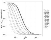
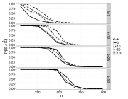
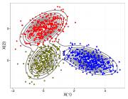
Figure 3: Left: false negative rate as a function of $\alpha$. Middle: overall screening error rate. Right: Final clustering based on relevant features.

In this section we give a brief example of the proposed method. First, we show the type II error (false negative rate) of the dip test as a function of $\alpha$. We use a version of the test implemented in the R package diptest. We take $P=\frac{1}{2}\mathcal{N}(0,1)+\frac{1}{2}\mathcal{N}(4,1)$. For a range of values for $n$, we draw $n$ samples from the mixture $10000$ times. The left plot in Figure 3 shows the fraction of times the dip test failed to detect multimodality at the specified values for $\alpha$. The increase in the sample size required for a certain power appears to be at most logarithmic in $1/\alpha$.

We show the overall error rate of the support estimation procedure in the middle plot in Figure 3 for the following multivariate distribution. For given values of $d$ and $s$, we use the Gaussian mixture $\frac{1}{2}\mathcal{N}(0,I)+\frac{1}{2}\mathcal{N}(4\mu_{s,d},I)$, where $\mu_{s,d}\in\mathbb{R}^{d}$ contains $s$ ones followed by $d-s$ zeroes, so that the true support is $S=\{1,\ldots,s\}$. The plot shows the fraction of times the estimated support $\widehat{S}$ did not exactly recover $S$ in $50$ replications of the experiment for each combination of parameters. We set $\alpha=0.1$ (and $\widetilde{\alpha}=\alpha/(nd)$). All the errors were due to incorrectly removing one of the multimodal dimensions – in other words, in every single instance it was the case that $\widehat{S}\subseteq S$. This is not surprising since the dip test can be conservative.

Finally, we apply the full method to a $d=20$ dimensional data set distributed in the first two dimensions according to the Gaussian mixture

$$\frac{2}{8}\mathcal{N}\left(\left(\begin{array}[]{c}0\\ 0\end{array}\right),\left(\begin{array}[]{cc}0.3&0.3\\ 0.3&2\end{array}\right)\right)+\frac{3}{8}\mathcal{N}\left(\left(\begin{array}[]{c}3\\ 0\end{array}\right),\left(\begin{array}[]{cc}0.6&-0.4\\ -0.4&1\end{array}\right)\right)+\frac{3}{8}\mathcal{N}\left(\left(\begin{array}[]{c}0\\ 5\end{array}\right),\left(\begin{array}[]{cc}0.45&0.45\\ 0.45&1.6\end{array}\right)\right),$$

and according to independent standard Gaussians in the remaining $d-s=18$ dimensions. We sample $n=1000$ points, and correctly recover the multimodal features using $\alpha=0.1$. The results of the subsequent mean shift clustering using $h=0.06$ are shown in Figure 3, along with contours of the true density.

7 Conclusion

We have proposed a new method for feature selection in high-dimensinal clustering problems. We have given bounds on the error rate in terms of clustering loss and Hausdorff distance. In future work, we will address the following issues:

1. The marginal signature assumption (A4) is quite strong. We do not know of any feature selection method for clustering that can succeed without some assumption like this. Either relaxing the assumption or proving that it is necessary is a top priority.

2. The bounds on clustering loss can probably be improved. This involves a careful study of the properties of the flow near cluster boundaries.

3. We conjecture that the Hausdorff bound is minimax. We think this can be proved using techniques like those in Romano (1988).

References

[1] Arias-Castro, Mason, Pelletier (2013). On the estimation of the gradient lines of a density and the consistency of the mean-shift algorithm. Manuscript.
[2] Audibert, Jean-Yves, and Alexandre B. Tsybakov. (2007). Fast learning rates for plug-in classifiers. The Annals of Statistics, 35, 608-633.
[3] Chacon, J. (2012). Clusters and water flows: a novel approach to modal clustering through Morse theory. arxiv:1212.1384.
[4] Chan, Yao-ban, and Peter Hall. (2010). Using evidence of mixed populations to select variables for clustering very high-dimensional data. Journal of the American Statistical Association, 105, 798-809.
[5] Cheng, Yizong. (1995). Mean shift, mode seeking, and clustering. IEEE Transactions on Pattern Analysis and Machine Intelligence, 17, 790-799.
[6] Comaniciu, Dorin, and Peter Meer. (2002). Mean shift: A robust approach toward feature space analysis. IEEE Transactions onPattern Analysis and Machine Intelligence, 24, 603-619.
[7] Einbeck, Jochen. (2011). Bandwidth selection for mean-shift based unsupervised learning techniques: a unified approach via self-coverage. Journal of pattern recognition research. 6, 175-192.
[8] Fan, Jianqing, and Jinchi Lv. (2008). Sure independence screening for ultrahigh dimensional feature space. Journal of the Royal Statistical Society: Series B, 70, 849-911.
[9] Guo, Jian, et al. (2010). Pairwise Variable Selection for High-Dimensional Model-Based Clustering. Biometrics, 66, 793-804.
[10] Hartigan, John A., and P. M. Hartigan. (1985). The dip test of unimodality. The Annals of Statistics, 13, 70-84.
[11] Muller, Dietrich Werner, and Gunther Sawitzki. (1991). Excess mass estimates and tests for multimodality. Journal of the American Statistical Association, 86, 738-746.
[12] Pan, W. and Shen, X. (2007). Penalized model-based clustering with application to variable selection. The Journal of Machine Learning Research, 8, 1145-1164.
[13] Raftery, Adrian E., and Nema Dean. (2006). Variable selection for model-based clustering. Journal of the American Statistical Association, 101, 168-178.
[14] Romano, J. (1988). On weak convergence and optimality of kernel density estimates of the mode. The Annals of Statistics 16, 629-647.
[15] Sriperumbudur, Bharath K., et al. (2009). Kernel Choice and Classifiability for RKHS Embeddings of Probability Distributions. NIPS.
[16] Sun, W., Wang, J. and Fang, Y. (2012). Regularized k-means clustering of high-dimensional data and its asymptotic consistency. Electronic Journal of Statistics, 6, 148-167.
[17] Wand, M. P., Duong, T. and Chacon, J. (2011). Asymptotics for general multivariate kernel density derivative estimators. Statistica Sinica, 21, 807-840.
[18] Witten, Daniela M., and Robert Tibshirani. (2010). A framework for feature selection in clustering. Journal of the American Statistical Association, 105, 713-726.
Appendix
Proof of Lemma 5. Let and be the gradient and Hessian of and let and be the gradient and Hessian of . Let be a mode of and let be a closed ball around where . The ball excludes any other mode of since . Expanding at we have