Signal processing on graphs: Transforms and tomograms

Abstract

Using projections on the (generalized) eigenvectors associated to matrices that characterize the topological structure, several authors have constructed generalizations of the Fourier transform on graphs. By exploring mappings of the spectrum of these matrices we show how to construct more general transforms, in particular wavelet-like transforms on graphs. For time-series, tomograms, a generalization of the Radon transforms to arbitrary pairs of non-commuting operators, are positive bilinear transforms with a rigorous probabilistic interpretation which provide a full characterization of the signals and are robust in the presence of noise. Here the notion of tomogram transform is also extended to signals on arbitrary graphs.

Keywords: Graph signals, Graph-transforms, Tomograms

I Introduction

I-A Signal transforms for time series: Linear, quasi-distributions and tomograms

The traditional field of signal processing deals mostly with the analysis of time series. Signal processing of time series relies heavily on integral transforms [1] [2]. Three types of transforms have been used: linear, bilinear and tomograms. Among the linear transforms Fourier and wavelets are the most popular. The Fourier transform extracts the frequency components of the signal and the wavelets its multiscale nature. However, this is achieved at the expense of the time information, in the sense that the time location of the frequency components and of the scale features is lost in the process. This motivated the development of bilinear transforms like the time-frequency Wigner-Ville [4] [5] or the frequency-scale Bertrand [6] [7] quasidistributions. The aim of the Wigner-Ville transform was to provide joint information on the time-frequency plane, which is important because in many applications (biomedical, seismic, radar, etc.) the signals are of finite (sometimes very short) duration. However, the oscillating cross-terms in the Wigner–Ville and other quasidistributions [8] [9] [10] make the interpretation of the transformed signals a difficult matter. Even when the average of the cross-terms is small, their amplitude may be greater than the signal in time–frequency regions that carry no physical information.

The difficulties with the physical interpretation of quasidistributions arise from the fact that time and frequency (or frequency and scale) are noncommutative operator pairs. Hence, a joint probability density can never be defined. Even in the case of positive quasiprobabilities like the Husimi–Kano function [11] [12], an interpretation as a joint probability distribution is also not possible because the two arguments in the function are not simultaneously measurable random variables. More recently, a new type of strictly positive bilinear transform has been proposed [13] [3] [14], called a tomogram, which is a generalization of the Radon transform [15] to arbitrary noncommutative pairs of operators. The Radon–Wigner transform [16] [17] is a particular case of the noncommutative tomography technique. Being strictly positive probability densities, the tomograms provide a full characterization of the signal and are robust in the presence of noise.

A unified framework to characterize linear transforms, quasidistributions and tomograms was developed in Ref.[3]. In short, considering a signal $f(t)$ as a vectors $\left|f\right\rangle$ in a subspace $\mathcal{N}$ of a Hilbert space $\mathcal{H}$, a family of unitary operators $U\left(\alpha\right)=e^{iB\left(\alpha\right)}$ and a reference vector $h$ in the dual $\mathcal{N}^{\ast}$ of $\mathcal{N}$ , a linear transform like Fourier or wavelet is

$$W_{f}^{(h)}(\alpha)=\langle U\left(\alpha\right)h\mid f\rangle$$ (1)

and a quasidistribution is

$$Q_{f}(\alpha)=\langle U\left(\alpha\right)f\mid f\rangle$$ (2)

To define the tomogram let, in the unitary operator $U\left(\alpha\right)=e^{iB\left(\alpha\right)}$, $B\left(\alpha\right)$ have the spectral decomposition $B\left(\alpha\right)=\int XP\left(X\right)dX$. Then

$$P\left(X\right)\circeq\left|X\right\rangle\left\langle X\right|$$

denotes the projector on the (generalized) eigenvector $\left\langle X\right|\in\mathcal{N}^{\ast}$ of $B\left(\alpha\right)$. The tomogram is

$$M_{f}^{(B)}(X)=\left\langle f\right|P\left(X\right)\left|f\right\rangle=\left\langle f\right|\left.X\right\rangle\left\langle X\right.\left|f\right\rangle=\left|\left\langle X\right.\left|f\right\rangle\right|^{2}$$ (3)

The tomogram $M_{f}^{(B)}(X)$ is the squared amplitude of the projection of the signal $\left|f\right\rangle\in\mathcal{N}$ on the eigenvector $\left\langle X\right|\in\mathcal{N}^{\ast}$ of the operator $B\left(\alpha\right)$. Therefore it is positive. For normalized $\mid f\rangle$,

$$\langle f\mid f\rangle=1$$

the tomogram is normalized

$$\int M_{f}^{(B)}\left(X\right)\,dX=1$$ (4)

and may be interpreted as a probability distribution on the set of generalized eigenvalues of $B\left(\alpha\right)$, that is, as the probability distribution for the random variable $X$ corresponding to the observable defined by the operator $B\left(\alpha\right)$.

For example, if the unitary $U\left(\alpha\right)$ is generated by $B_{F}\left(\overrightarrow{\alpha}\right)=\alpha_{1}t+i\alpha_{2}\frac{d}{dt}$ and $h$ is a (generalized) eigenvector of the time-translation operator, the linear transform $W_{f}^{(h)}(\alpha)$ is the Fourier transform. For the same $B_{F}\left(\overrightarrow{\alpha}\right)$, the quasi-distribution $Q_{f}(\alpha)$ is the ambiguity function and the Wigner–Ville transform [4] [5] is the quasi-distribution $Q_{f}(\alpha)$ for the following $B-$operator

$$B^{(WV)}(\alpha_{1},\alpha_{2})=-i2\alpha_{1}\frac{d}{dt}-2\alpha_{2}t+\frac{\pi\left(t^{2}-\frac{d^{2}}{dt^{2}}-1\right)}{2}\,$$ (5)

The wavelet transform is $W_{f}^{(h)}(\alpha)$ for $B_{W}\left(\overrightarrow{\alpha}\right)=\alpha_{1}D+i\alpha_{2}\frac{d}{dt}$, $D$ being the dilation operator $D=-\frac{1}{2}\left(it\frac{d}{dt}+i\frac{d}{dt}t\right)$. The wavelets $h_{s,\,\tau}(t)$ are kernel functions generated from a basic wavelet $h(\tau)$ by means of a translation and a rescaling $(-\infty<\tau<\infty,$ $s>0)$:

$$h_{s,\,\tau}(t)=\frac{1}{\sqrt{s}}\,h\left(\frac{t-\tau}{s}\right)$$ (6)

using the operator

$$U^{(A)}(\tau,s)=\exp(i\tau\hat{\omega})\exp(i\log\,sD),$$ (7)

$$h_{s,\tau}(t)=U^{(A)\dagger}(\tau,s)h(t).$$ (8)

The Bertrand transform [6] [7] is the quasi-distribution $Q_{f}(\alpha)$ for $B_{W}$. Linear, bilinear and tomogram transforms are related to one another [3].

As shown before, tomograms are obtained from projections on the eigenstates of the $B$ operators. These operators may be linear combinations of different (commuting or noncommuting) operators,

$$B=\mu O_{1}+\nu O_{2}$$

meaning that the tomogram explores the signal along lines in the plane $\left(O_{1},O_{2}\right)$. For example for

$$B\left(\mu,\nu\right)=\mu t+\nu\omega=\mu t+i\nu\frac{d}{dt}$$

the tomogram is the expectation value of a projection operator with support on a line in the time–frequency plane

$$X=\mu t+\nu\omega$$ (9)

Therefore, $M_{f}^{(S)}\left(X,\mu,\nu\right)$ is the marginal distribution of the variable $X$ along this line in the time–frequency plane. The line is rotated and rescaled when one changes the parameters $\mu$ and $\nu$. In this way, the whole time–frequency plane is sampled and the tomographic transform contains all the information on the signal. The probabilistic nature of the tomogram implies that, in contrast with quasi-distributions, the information thus obtained is robust and unambiguous. Tomograms associated to linear combinations of time with the generators of the conformal group ($i\nu\frac{d}{dt};i\left(t\frac{d}{dt}+\frac{1}{2}\right);i\left(t^{2}\frac{d}{dt}+t\right)$) and several other known operators have been explored [14].

By providing a robust extraction of compound signal features, tomograms have been useful in denoising, component separation and structure identification [18] [19] [20] [21] [22] [23].

I-B Signals on graphs

Social and economic networks, information networks, power grids, biological networks, etc. generate large sets of raw data from which, in general, only a detailed analysis may extract useful information. A first step is the construction of the appropriate signal transforms.

From the graph point of view a time series is a signal on a one-dimensional directed graph with vertices labelled by the times $\left(t_{0},t_{1},t_{2},\cdots\right)$ and the edges connecting $t_{k+1}$ to $t_{k}$. That is, the adjacency matrix $\mathbf{A}$ of a time series is, in general

$$\mathbf{A}=\left(\begin{array}[]{ccccc}0&0&0&0&\cdots\\ 1&0&0&0&\cdots\\ 0&1&0&0&\cdots\\ 0&0&1&0&\cdots\\ \vdots&\vdots&\vdots&\vdots&\cdots\end{array}\right)$$ (10)

or, for a time-periodic signal

$$\mathbf{A}=\left(\begin{array}[]{cccccc}0&0&0&\cdots&0&1\\ 1&0&0&\cdots&0&0\\ 0&1&0&\cdots&0&0\\ 0&0&1&\cdots&0&0\\ \vdots&\vdots&\vdots&\vdots&0&0\\ 0&0&0&0&1&0\end{array}\right)$$ (11)

As discussed before, signal transforms for a time series are projections on a set of eigenvectors of some linear operator. These operators are not arbitrary, but chosen to extract particular features of the signal that is being analyzed. The Fourier transform looks for periodic features, wavelets for multiscale features, etc. Likewise, useful information from signals on arbitrary graphs may be obtained from projections on sets of vectors associated to suitably chosen linear operators. For the time-periodic signal, it is easy to see that the discrete Fourier transform is the projection on the eigenvectors of the adjacency matrix (11). Therefore one may define the graph Fourier transform for an arbitrary graph as the projection on the eigenvectors (or on the generalized eigenvectors of the Jordan decomposition) of the adjacency matrix. This was the point of view taken by some authors [24] to develop a theory of discrete signal processing on graphs. However this choice is not unique because, for the time series network other matrices have the same spectrum, for example the Laplacian matrix

$$\mathbf{L}=\mathbf{D-A}$$

$\mathbf{D}$ being the degree matrix, which for the time series is the identity. Hence the graph Fourier transform might as well be defined as a projection on the generalized eigenvectors of the Laplacian matrix [25] [26]. This operator point of view allows not only to generalize the notion of transforms but also the notions of filtering and other general linear operations on graph signals.

II Signal transforms and tomograms on graphs

Here a generalization of the notions of linear transform and tomogram for signals on graphs will be developed. Generalization of the notion of bilinear transform will not be dealt with because, already for time series, it leads to difficult interpretation problems.

II-A Graph transforms

Let $G=(\mathcal{V},\mathbf{A})$ be a graph, with $\mathcal{V}=\{v_{0},\ldots,v_{N-1}\}$ the set of vertices and $\mathbf{A}$ the weighted adjacency matrix. Each matrix element $\mathbf{A}_{n,m}$ is the weight of a directed edge from $v_{m}$ to $v_{n}$ which can take arbitrary real or complex values. $\mathcal{N}_{n}=\{m\mid\mathbf{A}_{n,m}\neq 0\}$ is the neighborhood of $v_{n}$ and a graph signal is a map $\mathbf{f}=\left\{f_{n}\right\}$ from the set $\mathcal{V}$ of vertices into the set of complex numbers $\mathbb{C}$, each element $f_{n}$ being indexed by the vertex $v_{n}$.

Other useful matrices are:

- The degree matrix $\mathbf{D}$: a diagonal matrix listing the degree of the vertices

- The Laplacian matrix: $\mathbf{L}=\mathbf{D}-\mathbf{A}$

- The symmetrically normalized Laplacian matrix: $\mathbf{L}^{\prime}\mathbf{=D}^{-\frac{1}{2}}\mathbf{LD}^{-\frac{1}{2}}$

- The random walk matrix: $\mathbf{W}=\mathbf{AD}^{-1}$

- The lazy random walk matrix: $\mathbf{W}^{\prime}=\left(\mathbf{I}+\mathbf{AD}^{-1}\right)/2$

- The incidence matrix $\nabla$: is the $m\times N$ matrix ($m$=no. edges, $N$=no. of vertices) given by

$$\nabla_{e,v}=\left\{\begin{array}[]{cccc}1&\text{if}&e=\left(v,w\right)&\text{and }v<w\\ -1&\text{if}&e=\left(v,w\right)&\text{and }v>w\\ 0&&\text{otherwise}&\end{array}\right.$$

- The edge adjacency matrix: is a $m\times m$ matrix determined by the adjacencies of edges

$${}^{e}\mathbf{A}_{i,j}\mathbf{=}\left\{\begin{array}[]{ll}1&\text{if edges i and j are adjacent}\\ 0&\text{otherwise}\end{array}\right.$$

These matrices have been used in the past mostly to characterize the topological structure of networks, for vertex clustering, detection of communities, etc. [27] [28] [29] [30] [31]. Here they will be considered as operators which generate a set of (generalized) eigenvectors to project the signals on graphs.

Fourier-like transforms

Denote any one of these matrices by $\mathbf{M}$. The matrices $\mathbf{M}$ act on the space of graph signals by

$$f\rightarrow\widetilde{f}_{n}=\sum_{m}\mathbf{M}_{n,m}f_{m}=\sum_{m\in\mathcal{N}_{n}}\mathbf{M}_{n,m}f_{m}.$$ (12)

When the matrix $\mathbf{M}$ is the adjacency matrix this operation generalizes the notion of time shift, when time sequences are looked at as forward-connected graphs.

For many real-world datasets the matrices $\mathbf{M}$ are not diagonalizable. In those cases, to obtain a suitable set of expansion vectors one may either use the symmetric combinations $\mathbf{MM}^{T}$ and $\mathbf{M}^{T}\mathbf{M}$ to generate an expansion basis or, alternatively, use the block-diagonal Jordan decomposition of $\mathbf{M}$.

$$\mathbf{M}=VJV^{-1}$$ (13)

$$J=\begin{pmatrix}J_{R_{0,0}}(\lambda_{0})&&\\ &\ddots&\\ &&J_{R_{M-1,D_{M-1}}}(\lambda_{M-1})\end{pmatrix}$$ (14)

with Jordan blocks associated to the eigenvalues of $\mathbf{M}$

$$J_{r_{m,d}}(\lambda_{m})=\begin{pmatrix}\lambda_{m}&1&&\\ &\lambda_{m}&\ddots&\\ &&\ddots&1\\ &&&\lambda_{m}\end{pmatrix}$$ (15)

The columns of the matrix $V$, that brings $\mathbf{M}$ to its Jordan normal form, are the eigenvectors

$$(\mathbf{M}-\lambda_{m}\mathbf{1})\mathbf{v}_{m,d,0}=0$$ (16)

and the generalized eigenvectors of the Jordan chain

$$(\mathbf{M}-\lambda_{m}\mathbf{1})\mathbf{v}_{m,d,r}=\mathbf{v}_{m,d,r-1}$$ (17)

of $\mathbf{M}$. These vectors may then be used to project the signals on the graph and, considering the graph signal $\mathbf{f}$ as a column vector, the $\mathbf{M-}$transform is then

$$\mathbf{\widehat{f}}=V^{-1}\mathbf{f}$$ (18)

with inverse transform

$$\mathbf{f}=V\mathbf{\widehat{f}}$$ (19)

The problem with this decomposition lies in the fact that in general the set of generalized eigenvectors do not form an orthogonal basis. Therefore it is sometimes more convenient to use $\mathbf{MM}^{T}$ and $\mathbf{M}^{T}\mathbf{M}$ to generate the expansion basis, leading to what we will call the $\mathbf{MM}^{T}-$ or $\mathbf{M}^{T}\mathbf{M-}$transform.

Wavelet-like transforms

The definition of wavelet-like transforms for graphs requires a more elaborate construction. For time series the affine wavelets use, in Eq. (1), an operator $U\left(\alpha\right)$ consisting of the product of a translation and a scale transformation which acts on a fixed reference signal (the mother wavelet $h_{0}\left(t\right)$), namely

$$h_{s,a}\left(t\right)=U\left(s,a\right)h_{0}\left(t\right)=e^{\log s\left(t\frac{d}{dt}+\frac{1}{2}\right)}e^{a\frac{d}{dt}}h_{0}\left(t\right)=\sqrt{s}h_{0}\left(st+a\right)$$ (20)

Translation in the graph is easily generalized but it is not obvious how to generalize scale transformations. Hence we rewrite the wavelet transform in frequency space obtaining

$$f\left(a,s\right) = \int dth_{s,a}^{\ast}\left(t\right)f\left(t\right)=\int dt\left(e^{\log s\left(t\frac{d}{dt}+\frac{1}{2}\right)}e^{a\frac{d}{dt}}h_{0}^{\ast}\left(t\right)\right)f\left(t\right)$$ (21)

$$= \int d\omega\frac{e^{-i\frac{\omega}{s}a}}{\sqrt{s}}\widehat{h_{0}}^{\ast}\left(\frac{\omega}{s}\right)\widehat{f}\left(\omega\right)$$

$\widehat{h_{0}}$ and $\widehat{f}$ denoting the Fourier transforms of the mother wavelet and of the signal. One sees that the wavelet transform is represented as a sum over the Fourier spectrum $\Omega$ with the argument of the mother wavelet shifted from $\omega$ to $\frac{\omega}{s}$. The mapping $\omega\in\Omega\rightarrow\frac{\omega}{s}\in\Omega$ is a one-to-one onto mapping of $\Omega$ in $\Omega$. Therefore the natural generalization of the wavelet transform for graphs may be defined as a similar sum, with the spectrum label shift being one of the possible one-to-one onto mappings of the spectrum of the adjacency matrix (or of the Laplacian matrix).

Consider the Fourier-like transform on graphs and its inverse

$$f\left(i\right) = \sum_{\eta}\widehat{f}\left(\eta\right)\chi_{\eta}\left(i\right)$$

$$\widehat{f}\left(\eta\right) = \sum_{i}\chi_{\eta}\left(i\right)f\left(i\right)$$ (22)

$\chi_{\eta}\left(i\right)$ being an eigenvector of $A$ or $L$ (or a generalized eigenvector or an eigenvector of $A^{T}A$ or $L^{T}L$) and a localized ”mother wavelet”

$$h^{(k)}\left(i\right)=\delta_{k,i}$$ (23)

Then the wavelet-like transform on graphs would be

$$f\left(a,\widetilde{s}\right)=\sum_{\eta}\chi_{\widetilde{s}\left(\eta\right)}\left(k+a\right)\widehat{f}\left(\eta\right)$$ (24)

$\widetilde{s}\left(\eta\right)$ is not $\eta\rightarrow\frac{\eta}{s}$ because in general $\frac{\eta}{s}$ is not in $\Omega$. $\widetilde{s}$ would be a mapping in the set $\mathcal{S}$ of the possible one-to-one onto mappings of $\Omega$, $\widetilde{s}\in\mathcal{S}$.

The inverse wavelet transform is

$$\widehat{f}\left(\eta\right)=\frac{1}{\#\mathcal{S}}\sum_{a,\overset{\char 126\relax}{s}}\chi_{\widetilde{s}\left(\eta\right)}\left(a\right)f\left(a,\overset{\char 126\relax}{s}\right)$$ (25)

Hammond, Vandergheynst and Gribonval [32] have also attempted to generalize the notion of wavelet transform to graph signals. However, instead of the sum with the shifted arguments in the spectrum, they simply use a $\eta-$dependent weight on the sum with both the signal component $\overset{\curlywedge}{f}\left(\eta\right)$ and the eigenvector $\chi_{\eta}$ associated to the same spectral value $\eta$. Therefore their construction is more in the spirit of a superposition of Fourier-like transforms than of a wavelet transform.

A more general transform would be

$$f\left(a,C\right)=\sum_{\eta,\eta^{\prime}}C\left(\eta,\eta^{\prime}\right)\chi_{\eta^{\prime}}\left(a\right)\overset{\curlywedge}{f}\left(\eta\right)$$ (26)

For comparison with the time series case, this last construction would be similar to the case of the ”conformal wavelets” generated by $e^{\alpha\left(t^{2}\frac{d}{dt}+t\right)}e^{a\frac{d}{dt}}h_{0}\left(t\right)$.

II-B Graph tomograms

So far signals on graphs have been described either as vectors on vertex space or as projections of these vectors on the generalized eigenvectors of a particular matrix $\mathbf{M}$. Each particular matrix emphasizes a specific topological property of the graph. Tomograms attempt to obtain information about more than one property by projecting on the generalized eigenvectors of a matrix that interpolates between two distinct matrices $\mathbf{M}_{1}$ and $\mathbf{M}_{2}$. This parallels what for time series is achieved, for example, by the time-frequency tomogram.

When the vertex space has a meaningful physical interpretation it is useful to interpolate between one of the matrices $\mathbf{M}$ listed before and the matrix for which the vertex signal corresponds to a projection on its eigenvectors. For a graph with $N$ vertices, the vectors on vertex space may be considered as projections on the eigenvectors of a vertex operator

$$\mathbf{T}=\left(\begin{array}[]{ccccc}1&0&0&\vdots&0\\ 0&e^{i\frac{2\pi}{N}}&0&\vdots&0\\ 0&0&e^{i\frac{2\pi}{N}\times 2}&\vdots&0\\ \cdots&\cdots&\cdots&\ddots&\vdots\\ 0&0&0&\cdots&e^{i\frac{2\pi}{N}\times\left(N-1\right)}\end{array}\right)$$ (27)

Therefore the construction of a tomogram for graph signals would amount to finding an operator that interpolates between $T$ and $\mathbf{A}$. A solution could be the family of operators

$$B_{\alpha}=\left(1-\alpha\right)\mathbf{T}+\alpha\mathbf{M}$$ (28)

with $\alpha$ varying between $0$ and $1$, the tomogram being obtained by the projections of the signal on the eigenvectors of $B_{\alpha}$.

If $\mathbf{M}$ is the adjacency matrix $\mathbf{A}$, this construction, interpolating between $\mathbf{A}$ and the vertex operator $\mathbf{T}$, is for graphs, the analog of the time-frequency tomogram.

If the ordering of the vertices is arbitrary, the vertex operator has no special meaning and it is more useful to construct tomograms using two of the listed $\mathbf{M}$ matrices which, by construction, already contain meaningful information on the graph.

As discussed before, the reason why time and frequency cannot be simultaneously specified is because they correspond to a pair of non-commuting operators. This is the reason why bilinear transforms, like Wigner-Ville, are unreliable and it is also the main motivation for using tomogram transforms. In graphs also, the vertex description and the adjacency matrix projection are also incompatible specifications, because in general the $\mathbf{T}$ and $\mathbf{A}$ (or $\mathbf{L}$) matrices do not commute. It is in this sense, that, as recently stated [33], there is an uncertainty principle for graphs, that is, a fundamental trade-off between a signal localization on the graph and on its spectral domain.

II-C Tomograms and dynamics

The graph tomogram, as defined above, is appropriate for the study of a static network signal. If during the time evolution the graph structure stays the same, the time series associated to each vertex may simply be projected on the (generalized) eigenvectors as in the scalar case. However if the graph itself changes in time a more general framework must be used.

Consider a graph signal that evolves in (discrete) time. The corresponding graph would be, for each time $t$, a regular graph and each one of these graphs is forward-connected to the graph of the subsequent time. A vertex $\nu_{n}\left(t\right)$ at time $t$ connects to the vertex $\nu_{n}\left(t+1\right)$ at time $t+1$. This construction accommodates the possible disappearance of vertices. In that case such vertex $\nu_{n}\left(t\right)$ would not have any forward edges.

The construction of the $\mathbf{M-}$transforms and the graph tomograms will then proceed as before for the global adjacency matrix. To have a feeling for the kind of eigenvectors obtained for such adjacency matrices, consider a simple case of a finite-vertex circle graph with $N$ vertices symmetrically connected to nearest-neighbors and forward connected in periodic time with $\tau$ time steps. Then, at each time $t$, the subadjacency matrix $\mathbf{A}\left(t\right)$ is

$$\mathbf{A}\left(t\right)=\left(\begin{array}[]{cccccc}0&1&0&0&\vdots&1\\ 1&0&1&0&\vdots&0\\ 0&1&0&1&\vdots&0\\ 0&0&1&0&\vdots&0\\ \cdots&\cdots&\cdots&\cdots&\ddots&\vdots\\ 0&0&0&\cdots&1&0\end{array}\right)$$ (29)

Let, for definiteness and notational simplicity, $N=\tau=3$. Then the global $9\times 9$ adjacency matrix is

$$\mathbf{A}=\left(\begin{array}[]{ccccccccc}0&1&1&0&0&0&1&0&0\\ 1&0&1&0&0&0&0&1&0\\ 0&1&0&0&0&0&0&0&1\\ 1&0&0&0&1&1&0&0&0\\ 0&1&0&1&0&1&0&0&0\\ 0&0&1&0&1&0&0&0&0\\ 0&0&0&1&0&0&0&1&1\\ 0&0&0&0&1&0&1&0&1\\ 0&0&0&0&0&1&0&1&0\end{array}\right)$$ (30)

This matrix is a tensor product of matrices

$$\mathbf{A}=\left(\begin{array}[]{ccc}0&1&1\\ 1&0&1\\ 0&1&0\end{array}\right)\otimes\left(\begin{array}[]{ccc}0&0&1\\ 1&0&0\\ 0&1&0\end{array}\right)$$

with eigenvalues, respectively

$$\left(\begin{array}[]{c}-1\\ \frac{1}{2}\left(1+\sqrt{5}\right)\\ \frac{1}{2}\left(1-\sqrt{5}\right)\end{array}\right)\hskip 14.22636pt\text{and\hskip 14.22636pt}\left(\begin{array}[]{c}1\\ e^{i\frac{2\pi}{3}}\\ e^{i\frac{4\pi}{3}}\end{array}\right)$$ (31)

the eigenvectors of $\mathbf{A}$ being the tensor products of the eigenvectors of these matrices. The ”Fourier” transform of a dynamical graph signal will be the projection on these $9-$dimensional eigenvectors.

For the construction of the tomogram, the vertex operator $\mathbf{T}$, as in (27), is

$$\mathbf{T}=\left(\begin{array}[]{ccc}\mathbf{T}^{(3)}&\mathbf{0}&\mathbf{0}\\ \mathbf{0}&\mathbf{T}^{(3)}&\mathbf{0}\\ \mathbf{0}&\mathbf{0}&\mathbf{T}^{(3)}\end{array}\right)$$

where $\mathbf{T}^{(3)}$ is the $3\times 3$ matrix $\begin{array}[]{ccc}1&0&0\\ 0&e^{i\frac{2\pi}{3}}&0\\ 0&0&e^{i\frac{2\pi}{3}\times 2}\end{array}$.

III Illustrative examples

In this section we present some examples of the use of graph transforms and graph tomograms. The detailed economic and biological implications of the examples are beyond the scope of this paper. The examples are included only as an illustration of the concepts and also as a guide on how the graph formulation may be a powerful tool to analyze multivariate time series.

III-A A market network

An important problem in the design of portfolios or ETF’s is the classification of the dynamical behavior of the trading values of market products. Identifying clusters of products with similar dynamical behavior allows the design of simpler portfolios, by the selection of representative elements in each cluster. Here we analyze the daily closing equity prices of $301$ companies in the SP500 throughout the $250$ trading days of 2012. For the purpose of the calculations the companies are ordered by sectors. The company ticker symbols and GICS sector codes are listed in the Appendix.

From the daily returns

$$r\left(t\right)=\log S\left(t\right)-\log S\left(t-1\right)$$ (32)

$S\left(t\right)$ being the closing price at day $t$, one computes a dynamical distance between the company stocks $i$ and $j$ by

$$d_{ij}=\sqrt{\sum_{t=1}^{250}\left(r_{i}\left(t\right)-r_{j}\left(t\right)\right)^{2}}$$ (33)

the sum being over the $250$ trading days in 2012.

Now one computes the smallest non-zero $d_{ij}$ ($d_{\min}$) and an adjacency matrix $A$ with matrix elements $A_{ij}$ may be defined either by

$$A_{ij}^{\#}=\frac{d_{\min}}{d_{ij}}\left(1-\delta_{ij}\right)$$ (34)

or

$$A_{ij}^{\left(\beta\right)}=\left(1-\delta_{ij}\right)\exp\left(-\beta\left(d_{ij}-d_{\min}\right)\right)$$ (35)

The second form is sometimes the most convenient one because, by varying $\beta$, one obtains a multiscale analysis of the dynamical similarities of the companies. In Figs. 1 and 2 we show the color-coded adjacency matrices $A$ and $A^{\left(\beta=2\right)}$ that are obtained. One sees that the $A^{\left(\beta=2\right)}-$adjacency matrix provides a more detailed picture of the nature of correlations between the return behavior of these equities. From inspection of this matrix one already sees that although the strongest correlations are on the ”utilities” sector (GICS code 55), many other inter-sectors correlations do exist. The main purpose of the analysis is precisely to identify sets of companies with similar return behavior.

Figure 1: Color-coded adjacency matrix $A^{\#}$ for the 301 companies

Figure 2: Color-coded adjacency matrix $A^{\left(\beta\right)}$, $\beta=2$, for the 301 companies

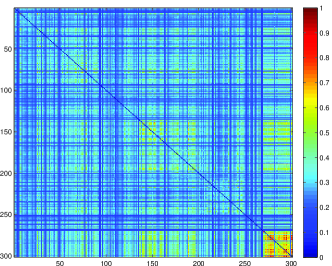
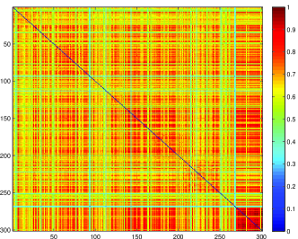
For the remaining of our calculations we will use the $A^{\left(\beta=2\right)}\circeq A$ as the adjacency matrix.

Now consider, as the signal on this graph, the yearly compound return

$$R_{i}=\prod_{t=1}^{250}\left(1+r_{i}\left(t\right)\right)$$ (36)

In Fig. 3 we compare the compound return $R_{i}$ of the companies with the absolute value of the projections of $R_{i}-\left\langle R_{i}\right\rangle$ on the eigenvectors of the adjacency $A$ and the Laplacian $L=D-A$ matrices. $\left\langle R_{i}\right\rangle$ is the mean value of the compound returns, which in this case was $1.1003$.

Figure 3: The compound returns $R_{i}$ and the absolute values of the projection of $R_{i}-\left\langle R_{i}\right\rangle$ on the eigenvectors of the adjacency and Laplacian matrices

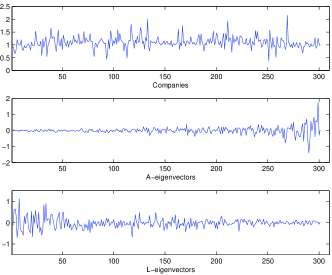
One sees that the projection on the $A-$eigenvectors (the $A-$transform) is the one that provides a better information compression by selecting a smaller number of dominant eigenvectors.

A standard spectral technique to find clusters in a graph is to look at the lowest non-zero eigenvalues in the spectrum of the Laplacian matrix, the corresponding eigenvectors leading (by K-means) to a division into clusters that minimizes the RatioCut [27]

$$RatioCut\left(C_{1},...,C_{K}\right)=\frac{1}{2}\sum_{k=1}^{K}\frac{W\left(C_{k},\overline{C_{k}}\right)}{\left|C_{k}\right|}$$

where $W\left(C_{k},\overline{C_{k}}\right)=\sum_{i\in C_{k},j\in\overline{C_{k}}}A_{ij}$, $\overline{C_{k}}$ is the complement of $C_{k}$ and $\left|C_{k}\right|$ is the number of elements in the cluster $C_{k}$.

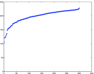
From Fig.4, where we have plotted the eigenvalues of the Laplacian matrix, one sees that in this case this criterium does not provide clear information on the cluster properties of the market network.

Figure 4: Eigenvalues of the Laplacian matrix

How the companies organize themselves into groups with similar return behavior is better understood by the examination of the $T-A$ tomogram (Fig.5). The figure is a contour plot of the absolute value of the projections of the compound return (Eq.36) on the eigenvectors of $B_{\alpha}=\left(1-\alpha\right)\mathbf{T}+\alpha\mathbf{A}^{\left(2\right)}$.

Figure 5: The $T-A$ tomogram

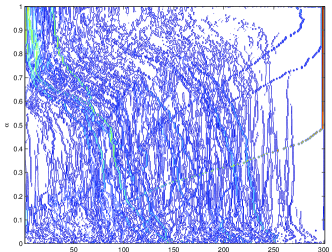
One sees how, starting from the compound return signal at $\alpha=0$, the contributions of the companies organize themselves into clusters on the way to the final projection on the $\mathbf{A}-$eigenvectors (at $\alpha=1$). The selection of clusters may be done by cutting the tomogram at diverse levels and reconstructing the components of the signal. The tomogram has a rigorous probabilistic interpretation and all the signal information is contained at each $\alpha$ level. Therefore the signal components (dynamical clusters) are reconstructed by linear combinations of the eigenvectors around each peak with the coefficients taken from the tomogram. As an example Fig. 6 shows the cut at $\alpha=0.85$ and Fig. 7 the reconstruction of the signal components around three of its peaks.

Figure 6: The $T-A$ tomogram cut at $\alpha=0.85$

Figure 7: The compound return and the absolute value of $R_{i}-\left\langle R_{i}\right\rangle$ for three different clusters in the tomogram

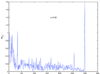
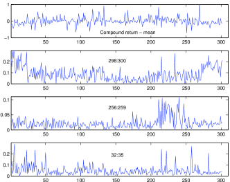
One sees how these distinct dynamical clusters have important contributions from different sectors. For example the last peak (components 298 to 300) is dominated by companies both in the utilities and the energy sector.

III-B A trophic network

In this example, to be studied in more detail elsewhere, we analyze a biological network for which two types of information are available. It concerns 12 fish species of the North Atlantic for which we have information both on their trophic relations and on their biomass evolution in the period 1976-2013. These species were selected for the availability of a relatively long biomass time series. The trophic relations, obtained from averaged stomach sampling are displayed in Fig. 8 and in the color-coded adjacency matrix $A_{\text{troph}}$ of Fig. 9.

Figure 8: North Sea Foodweb 12 species, directed and weighted

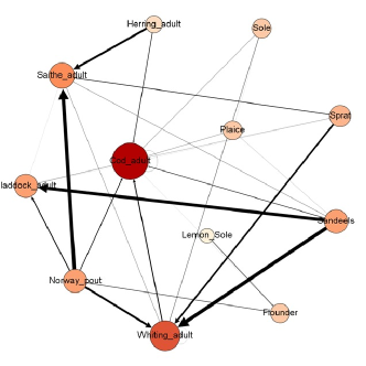
The ordered 12 species are: 1 = Cod adult; 2 = Whiting adult; 3 = Haddock adult; 4 = Saithe adult; 5 = Norway pout; 6 = Herring adult; 7 = Sprat; 8 = Sandeels; 9 = Plaice; 10 = Flounder; 11 = Sole; 12 = Lemon Sole.

Figure 9: Color-code trophic adjacency matrix $A_{\text{troph}}$ for the 12 fish species

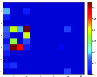
Notice that in the $A_{\text{troph}}$ matrix the lines do not sum up to one, because other species enter in the stomach data beyond the 12 considered here.

On the other hand, considering, for each biomass time series $b\left(t\right)$, the population growth rate as the most relevant variable [34]

$$r\left(t\right)=\log\left(\frac{b\left(t\right)}{b\left(t-1\right)}\right)$$ (37)

we define the $\Delta-$ delay distance function

$$d_{ij}^{\left(\Delta\right)}=\sqrt{\sum_{t=\Delta}^{38}\left(r_{i}\left(t\right)-r_{j}\left(t-\Delta\right)\right)^{2}}$$ (38)

The reason to consider time-delays for the growth rate distances is because in a trophic network the biomass is related to the other species offspring of previous years.

For each distance matrix, with elements $d_{ij}^{\left(\Delta\right)}$, we find the smallest nonzero element ($d_{\min}^{\left(\Delta\right)}$) and define biomass delayed adjacency matrices as

$$A_{ij}^{\left(\Delta\right)}=\frac{d_{\min}^{\left(\Delta\right)}}{d_{ij}^{\left(\Delta\right)}}$$ (39)

Fig. 10 displays the color-code one-year delayed biomass adjacency matrix.

Figure 10: Color-code one-year delayed biomass adjacency matrix

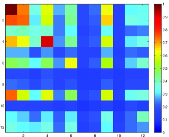
A simple inspection of Figs. 9 and 10 shows that the trophic and the biomass data do not contain the same information, which is to be expected since the biomass growth rate depends in many other factors besides predation. This is better seen in Fig.11 where we have normalized to one each column in the trophic matrix, and then compared the 28 nonzero elements with the corresponding elements in the $A_{ij}^{\left(\Delta\right)}$ matrices (also normalized to one).

Figure 11: Trophic versus growth rate adjacency matrices

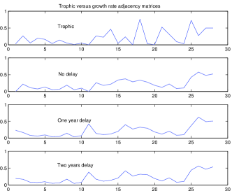
Although some partial trends might be similar, the general conclusion is that the biomass growth rate evolution seems to depend on many other factors, different from the trophic relations of these 12 species.

In the remaining of this subsection we will use the one-year delayed biomass growth rate and the tomographic analysis to exhibit the interspecies correlations. Fig. 12 shows a contour plot of the tomogram corresponding to the operator $B=\left(1-\alpha\right)T+\alpha A^{\left(1\right)}A^{\left(1\right)T}$. The signal that is projected on the eigenvectors of this operator is $R_{i}-\left\langle R_{i}\right\rangle$, $R_{i}$ being the compound growth rate over 36 years

$$R_{i}=\prod_{t=1}^{36}\left(1+r_{i}\left(t\right)\right)$$

The breaks that are observed in the contour plot result from the automatic ordering of the eigenvectors by ascending eigenvalue values. They are of no practical consequence, full information on the signal being kept at all $\alpha-$levels. One sees how, for $\alpha\neq 0$ the signal information is compressed in a small number of eigenvectors.

Figure 12: The tomogram corresponding to the operator $B=\left(1-\alpha\right)T+\alpha A^{\left(1\right)}A^{\left(1\right)T}$

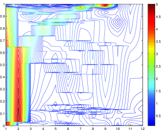
As in the market network example, cutting the tomogram at intermediate $\alpha$ levels, clustering dependency of the species is obtained. This will be reported in detail elsewhere. Here we only want to illustrate the use of the graph tools that have developed and the promising power of the graph formulation for the analysis of multivariate time series.

Appendix

Ticker symbols and GICS sector codes of the SP500 companies used in the example 3.1

APA(10); APC(10); BHI(10); CHK(10); CNX(10); COG(10); COP(10); CVX(10); DNR(10); DO(10); DVN(10); FTI(10); HAL(10); HES(10); HP(10); MRO(10); NBL(10); NOV(10); OXY(10); PXD(10); RDC(10); SLB(10); SWN(10); VLO(10); WMB(10); XOM(10); AA(15); APD(15); ARG(15); ATI(15); BLL(15); BMY(15); CAM(15); CF(15); CLF(15); DD(15); DOW(15); ECL(15); EMN(15); IFF(15); IP(15); MON(15); MUR(15); NEM(15); NUE(15); PPG(15); PX(15); SEE(15); VMC(15); X(15); APH(20); AVY(20); BA(20); CAT(20); CMI(20); CSX(20); DE(20); DHR(20); DNB(20); DOV(20); EFX(20); EMR(20); ETN(20); FDX(20); FLR(20); FLS(20); GD(20); GE(20); GWW(20); HON(20); IR(20); IRM(20); ITW(20); LLL(20); LMT(20); LUV(20); MAS(20); MMM(20); NOC(20); NSC(20); PBI(20); PH(20); PLL(20); R(20); RHI(20); ROK(20); RTN(20); TYC(20); UNP(20); UTX(20); AN(25); AZO(25); BBY(25); BIG(25); CCE(25); COH(25); DFS(25); DIS(25); DRI(25); F(25); FDO(25); GCI(25); GPC(25); GPS(25); HAR(25); HD(25); HOG(25); HOT(25); HRB(25); IGT(25); IPG(25); JCI(25); JCP(25); JWN(25); KMX(25); LEG(25); LEN(25); LOW(25); LTD(25); MCD(25); MHP(25); NKE(25); NWL(25); OMC(25); PCP(25); SHW(25); SNA(25); SWK(25); TGT(25); TIF(25); TJX(25); VFC(25); WHR(25); ADM(30); AVP(30); BFb(30); CAG(30); CCL(30); CL(30); CLX(30); CPB(30); CVS(30); DF(30); DPS(30); EL(30); GIS(30); HNZ(30); HRL(30); HSY(30); JEC(30); K(30); KMB(30); KO(30); KR(30); LO(30); M(30); MJN(30); MO(30); PEP(30); PG(30); PM(30); SJM(30); STZ(30); SWY(30); SYY(30); TAP(30); TSO(30); WAG(30); WMT(30); WPO(30); ABC(35); ABT(35); AET(35); AGN(35); BAX(35); BCR(35); BDX(35); BMS(35); BSX(35); CAH(35); CFN(35); CI(35); CVH(35); DGX(35); DVA(35); FRX(35); HSP(35); HUM(35); JNJ(35); LH(35); LLY(35); MCK(35); MDT(35); MKC(35); MRK(35); PFE(35); PKI(35); STJ(35); SYK(35); THC(35); TMO(35); UNH(35); VAR(35); WAT(35); WLP(35); AFL(40); AIG(40); AIZ(40); ALL(40); AXP(40); BAC(40); BBT(40); BEN(40); BK(40); BTU(40); C(40); CB(40); CBG(40); CMA(40); COF(40); FHN(40); GNW(40); GS(40); HIG(40); JPM(40); KEY(40); L(40); LM(40); LNC(40); LUK(40); MET(40); MMC(40); MTB(40); NBR(40); NYX(40); PGR(40); PNC(40); RF(40); SCHW(40); STI(40); STT(40); TMK(40); TRV(40); TSN(40); UNM(40); USB(40); WFC(40); WM(40); XL(40); A(45); AMD(45); CSC(45); EMC(45); FCX(45); FIS(45); GLW(45); GME(45); HPQ(45); HRS(45); IBM(45); JBL(45); JNPR(45); MA(45); MWV(45); TER(45); TSS(45); XRX(45); PCS(50); S(50); T(50); VZ(50); AEE(55); AEP(55); AES(55); CMS(55); CNP(55); D(55); DTE(55); DUK(55); ED(55); EIX(55); EQT(55); ETR(55); EXC(55); FE(55); GAS(55); NEE(55); NI(55); NU(55); PCG(55); PEG(55); PNW(55); POM(55); PPL(55); SCG(55); SRE(55); TE(55); TEG(55); TXT(55); WEC(55); XEL(55).

References

- [1] A. D. Poularikas (Ed.); The Transforms and Applications Handbook, CRC Press & IEEE Press, Boca Raton, Florida (1996).
- [2] K.-B. Wolf; Integral Transforms in Science and Engineering, Plenum Press, New York (1979).
- [3] M. A. Man’ko, V. I. Man’ko and R. Vilela Mendes; Tomograms and other transforms: A unified view, J. Phys. A: Math. and Gen.34 (2001) 8321-8332.
- [4] E. Wigner; On the quantum correction for thermodynamic equilibrium, Phys. Rev., 40 (1932) 749–759.
- [5] J. Ville; Théorie et applications de la notion de signal analytique, Cables et Transmission, 2 A (1948) 61–74.
- [6] J. Bertrand and P. Bertrand; A class of affine Wigner functions with extended covariance properties, J. Math. Phys., 33 (1992) 2515–2527.
- [7] P. Goncalvés and R. G. Baraniuk; A pseudo-Bertrand distribution for time–scale analysis, IEEE Signal Process. Lett. 3 (1996) 82–84.
- [8] L. Cohen; Generalized phase-space distribution functions, J. Math. Phys. 7 (1966) 781–806.
- [9] L. Cohen; Time–frequency distributions. A review, Proc. IEEE 77 (1989) 941–981.
- [10] S. Qian and D. Chen; Joint time–frequency analysis, Prentice-Hall, Englewood Cliffs, N. J. (1995).
- [11] K. Husimi; Some formal properties of the density matrix, Proc. Phys. Mat. Soc. Jpn, 22 (1940) 264–314.
- [12] Y. Kano; A new phase-space distribution function in the statistical theory of the electromagnetic field, J. Math. Phys. 6 (1965) 1913–1915.
- [13] V. I. Man’ko and R. Vilela Mendes; Noncommutative time–frequency tomography, Phys. Lett. A, 263 (1999) 53–59.
- [14] F. Briolle, V. I. Man’ko, B. Ricaud and R. Vilela Mendes; Non-commutative tomography: A tool for data analysis and signal processing, Journal of Russian Laser Research 33 (2012) 103-121.
- [15] S. R. Deans; The Radon Transform and Some of Its Applications, John Wiley & Sons, New York 1983.
- [16] J. C. Woods and D. T. Barry; Linear signal synthesis using the Radon–Wigner transform, IEEE Trans. Signal Process. 42 (1994) 2105–2111.
- [17] S. Granieri, W. D. Furlan, G. Saavedra, and P. Andrés; Radon–Wigner display: a compact optical implementation with a single varifocal lens, Appl. Opt. 36 (1997) 8363–8369.
- [18] F. Briolle, R. Lima, V. I. Man’ko and R. Vilela Mendes; A tomographic analysis of reflectometry data I: Component factorization, Meas. Sci. Technol. 20 (2009) 105501.
- [19] F. Briolle, R. Lima and R. Vilela Mendes; A tomographic analysis of reflectometry data II: The phase derivative, Meas. Sci. Technol. 20 (2009) 105502.
- [20] F Clairet, F Briolle, B Ricaud and S Heuraux; New signal processing technique for density profile reflectometry on Tore Supra, Rev. Sci. Instrum. 82 (2011) 083502.
- [21] B. Ricaud, F. Briolle and F. Clairet; Analysis and separation of time-frequency components in signals with chaotic behavior, arXiv:1003.0734.
- [22] C. Aguirre, P. Pascual, D. Campos and E.Serrano; Single neuron transient activity detection by means of tomography, BMC Neuroscience 2011, 12(Suppl 1):P297
- [23] C. Aguirre and R. Vilela Mendes; Signal recognition and adapted filtering by non-commutative tomography, IET Signal Processing 8 (2014) 67-75.
- [24] A. Sandryhaila and J. F. Moura; Discrete signal processing on graphs, IEEE Trans. on Signal Processing 61 (2013) 1644-1656.
- [25] B. A. Miller, N. T. Bliss and P. J. Wolfe; Towards signal processing theory for graphs and non-Euclidean data, in Proc. ICASSP, pp.5414-5417, 2010.
- [26] D. I. Shuman et al.; The emerging field of signal processing on graphs. Extending high-dimensional data analysis to networks and other irregular domains, IEEE Signal Processing Mag. 30 (2013) 83-98.
- [27] U. Von Luxburg; A tutorial on spectral clustering, Stat. Comp. 17 (2007) 395-416.
- [28] F. Krzakala, C. Moore, E. Mossel, J. Neeman, A. Sly and L. Zdeborova; Spectral redemption in clustering sparse networks, doi/10.1073/pnas.1312486110.
- [29] R. Nadakuditi and M. Newman; Graph spectra and the detectability of community structure in networks, Phys. Rev. Lett. 108 (2012) 188701.
- [30] K. Hashimoto; Zeta functions of finite graphs and representation of p-adic groups, Adv. Studies in Pure Math. 15 (1989) 211-280.
- [31] M. Newman; Finding community structure in networks using the eigenvectors of matrices, Phys. Rev. E 74 (2006) 036104.
- [32] D. K. Hammond, P. Vandergheynst and R. Gribonval; Wavelets on graphs via spectral graph theory, Appl. Comput. Harmon. Anal. 30 (2011) 129-150.
- [33] A. Agaskar and YueM. Lu; A Spectral Graph Uncertainty Principle, IEEE Trans. on Information Theory 59 (2013) 4338-4356.
- [34] H-S. Niwa; Random-walk dynamics of exploited fish populations, ICES Journal of Marine Science, 64 (2007) 496–502.