Robust a Posteriori Error Estimates for HDG method for Convection-Diffusion Equations

Abstract.

We propose a robust a posteriori error estimator for the hybridizable discontinuous Galerkin (HDG) method for convection-diffusion equations with dominant convection. The reliability and efficiency of the estimator are established for the error measured in an energy norm. The energy norm is uniformly bounded even when the diffusion coefficient tends to zero. The estimators are robust in the sense that the upper and lower bounds of error are uniformly bounded with respect to the diffusion coefficient. A weighted test function technique and the Oswald interpolation are key ingredients in the analysis. Numerical results verify the robustness of the proposed a posteriori error estimator.

1. Introduction

Given a bounded, polyhedral domain $\Omega\subset R^{d}(d=2,3)$, we consider the convection-diffusion equations

$$-\epsilon\Delta u+\boldsymbol{\beta}\cdot\nabla u+cu= \;f\quad\text{ in $\Omega$, }$$ (1.1a)

$$u= \;g\quad\text{ on $\partial\Omega$.}$$ (1.1b)

The data and the right-hand sides in (1.1) satisfy the following assumptions:

1. $0<\epsilon\leq 1$.

2. $\boldsymbol{\beta}\in W^{1,\infty}(\Omega)^{d}$, $c\in L^{\infty}(\Omega)$, $f\in L^{2}(\Omega)$ and $g\in H^{\frac{1}{2}}(\partial\Omega)$.

3. $c-\frac{1}{2}{\rm div}\boldsymbol{\beta}\geq 0$.

4. There is a function $\psi\in W^{1,\infty}(\Omega)$ and a positive constant $b_{0}$ such that $\boldsymbol{\beta}\cdot\nabla\psi\geq b_{0}$.

Assumption (A1) includes the case of the convection-dominated regime. According to [4], Assumption (A4) is satisfied if $\boldsymbol{\beta}$ has no closed curves and $|\boldsymbol{\beta}(x)|\neq 0\text{ for all }x\in\Omega$.

It is well known that solutions of (1.1) may develop layers (cf. [24, 29]). In particular, the solutions may have singular interior layer of width $O(\sqrt{\epsilon})$ or outflow layer of width $O(\epsilon)$. Standard numerical methods, e.g., standard finite element method or central finite difference method, are not robust when the quantity $\epsilon/\|\boldsymbol{\beta}\|_{L^{\infty}(\Omega)}$ is small compared to the mesh size. In order to stabilize the numerical method, several remedies are proposed for addressing the issue, for instance, streamline diffusion method [6], residual free bubble methods [7, 8, 10], local projection schemes [37], subgrid scale method [16, 5], continuous interior penalty (CIP) methods [11, 12], discontinuous Galerkin methods [4, 32, 33], and recently discontinuous Petrov-Galerkin (DPG) methods [9, 13, 23], HDG method [31] and the first order least squares method [15]. One can refer to [40, 44] for more other stabilization techniques. But in order to capture the potential interior or outflow layer of the solutions to the problem (1.1), the local Péclet number $P_{e}=h\|\boldsymbol{\beta}\|_{L^{\infty}(\Omega)}/\epsilon$ near the layers should be small enough, where $h$ is the mesh size. Hence it would be quite expensive for the stabilized numerical methods used on the quasi-uniform mesh to capture the layers when $\epsilon$ is small. If the mesh in the vicinity of the layers can be locally refined, the cost of numerical computations could be reduced. Therefore the adaptive finite element method is a natural choice for the efficient solution of convection-diffusion equations with dominant convection.

The adaptive finite element method based on a posteriori error estimates have been well established for second-order elliptic problems (cf. [2, 47]). In recent years the a posteriori error estimates are also extended to convection-diffusion equation. An early attempt was proposed by Eriksson and Johnson in [26], using regularization and duality techniques. Verfürth [48] proposed semi-robust estimators in the energy norm for the standard Galerkin approximation and the streamline upwind Petrov-Galerkin (SUPG) discretization. In [49] Verfürth improved his results by giving the estimates which are robust with dominant convection in a norm incorporating the standard energy norm and a dual norm of the convective derivative. Very recently, Tobiska and Verfürth [45] derived the same robust a posteriori error estimators for a wide range of stabilized finite element methods such as streamline diffusion methods, local projection schemes, subgrid scale technique and CIP method. However, the energy norm of error used in Verfürth’s estimates is defined through a dual norm which is not easy to compute. Sangalli [41] proposed different norms for the a posteriori error estimates that allow for robust estimators, but the analysis is only valid in the one dimensional case. As to other approaches for the robust error estimations, one can refer to [50] for mixed finite element methods, [51] for cell-centered finite volume scheme, [3] for nonconforming finite element method, [27, 28, 42, 52] for interior penalty discontinuous Galerkin method.

Discontinuous Galerkin (DG) methods have several attractive features compared with conforming finite element methods. For example, DG methods have elementwise conservation of mass, and they work well on arbitrary meshes. However, the dimension of the approximation DG space is much larger than the dimension of the corresponding conforming space. The HDG method [18, 19, 36] was recently introduced to address this issue. HDG methods retain the advantages of standard DG methods and result in significant reduced degrees of freedom. New variables on all interfaces of mesh are introduced such that the numerical solution inside each element can be computed in terms of them, and the resulting algebraic system is only due to the unknowns on the skeleton of the mesh. In [31], the HDG method was proposed and analyzed for the problem (1.1) on shape-regular mesh. The stabilization parameter of the HDG method in [31] can be determined clearly, meanwhile the penalty parameters of the DG schemes [4] need to be chosen empirically. Moreover, the condition number of stiffness matrix of a new way of implementing HDG method in [31] was proven to be bounded by $O(h^{-2})$ and independent of the diffusion coefficient $\epsilon$. These properties are important for the efficient solution of the problem (1.1) and encourage us to consider the corresponding HDG method on adaptive meshes.

The a posteriori error analysis for the HDG method for second order elliptic problems has been presented in [20, 21], where the error incorporates only the flux and a postprocessed solution used in the estimators. To our best knowledge, no a posteriori error estimates for the HDG discretizations of convection-diffusion problems have been studied in the literature so far. In this work, our objective is to show that the HDG scheme proposed in [31] gives rise to robust a posteriori error estimates for the problem (1.1). In comparison with the postprocessing technique utilized in [50, 20, 21], we establish the estimators without any postprocessed solution since the solution of (1.1) is always not smooth and there is no superconvergence result for the HDG method when $\epsilon\ll 1$.

We notice that the a posteriori error estimators for nonconforming finite element method [3] and interior penalty DG method [27, 28] are only semi-robust in the sense that they yield lower and upper bounds of the error which differ by a factor equal at most to $\mathcal{O}(\epsilon^{-1/2})$. In [42, 52], the a posteriori error estimator is robust in the sense that the ratio of the constants in the upper and lower bounds of error is independent of the diffusion coefficient. However, the energy norm of error in [42, 52] contains the jump term $\left(h_{F}\epsilon^{-1}\|\llbracket u_{h}\rrbracket\|^{2}_{0,F}\right)^{1/2}$ on each interior interface of meshes. In contrast, the a posteriori error estimator in this paper is robust based on the energy norm in (2.9), which contains a jump term $\left(\gamma_{F}\|\llbracket u_{h}\rrbracket\|^{2}_{0,F}\right)^{1/2}$ instead. One can refer to (2.7) for the definition of paparemeter $\gamma_{F}$. So, our a posteriori error estimator will not enlarge the error estimate too much as the error estimator in [42, 52], when the mesh size is not small compared with the diffusion coefficient.

To derive the reliability and efficiency of the estimators for the error measured in an energy norm which incorporates a scaling flux and the scalar solution of the HDG discretization, two techniques are utilized. The first one is to use the Oswald interpolation operator to approximate a discontinuous polynomial by a continuous and piecewise polynomial function and to control the approximation by the jumps (cf. [34, 35]). For most of a posteriori error estimates mentioned above (e.g. [49, 50, 45, 27, 28, 42, 52]), the analysis only gives the estimates for the energy error without $L^{2}$-error of the scalar solution when $c-\frac{1}{2}{\rm div}\boldsymbol{\beta}=0$. The second one is to address this issue and to employ a weighted function to derive the estimates for the error which contains $L^{2}$-error of the scalar solution. This idea goes back to Nävert’s work [46] for convection-diffusion problems and was used to obtain the $L^{2}$-stability of the original DG method for pure hyperbolic equation [39] and extended to convection-diffusion equations using the IP-DG method [30, 4], the HDG method [31] and the first order least squares method [15].

In the numerical experiments, the convection-diffusion problems with interior or outflow layers are tested based on the proposed a posteriori error estimator. The robustness of the a posteriori error estimator based on the HDG method is observed for the problems with different diffusion coefficient. We also find that the convergence of the adaptive HDG method is almost optimal, i.e., the convergence rate is almost $O(N^{-s})$, where $N$ is the number of elements, $s$ depends on the polynomial order $p$.

The outline of the paper is as follows: We introduce some notations, the HDG method, a posteriori error estimator and main results in the next section. In section 3, we collect some auxiliary results for analysis. Section 4 and section 5 are devoted to the proofs of reliability and efficiency, respectively. In the final section, we give some numerical results to confirm our theoretical analysis.

2. Notation, HDG method, error estimator, and main results

In this section, we begin with some basic notation and hypotheses of meshes. Secondly, we introduce the HDG method for (1.1) in [31]. Then, we define the corresponding a posteriori error estimator. Finally, we give the main results of reliability and efficiency.

2.1. Notation and the mesh

Let $\mathcal{T}_{h}$ be a conforming, shape-regular simplicial triangulation of $\Omega$. For any element $T\in\mathcal{T}_{h}$, $\partial{T}$ denotes the set of its edges in the two dimensional case and of its faces in the three dimensional case. Elements of $\partial{T}$ will be generally referred to as faces, regardless of dimension, and denoted by $F$. We define $\partial\mathcal{T}_{h}:=\{\partial T:T\in\mathcal{T}_{h}\}$. We denote by $\mathcal{E}_{h}$ the set of all faces in the triangulation (the skeleton), while the set of all interior (boundary) faces of the triangulation will be denoted $\mathcal{E}_{h}^{0}$ ($\mathcal{E}_{h}^{\partial}$). Correspondingly, we refer to ${\mathcal{N}}_{h}$ the set of vertices and to ${\mathcal{N}}_{h}^{0}$ the set of interior vertices. For any $T\in\mathcal{T}_{h}$, let $h_{T}$ be the diameter of element $T$. Similarly, for any $F\in{\mathcal{E}}_{h}$, we define $h_{F}:={\rm diam}(F)$. Throughout this paper, we use the standard notations and definitions for Sobolev spaces (see, e.g., Adams[1]). We also use the notation $\|\cdot\|_{0,D}$ and $\|\cdot\|_{0,\Gamma}$ to denote the $L^{2}$-norm on the elements $D$ and faces $\Gamma$, respectively.

2.2. The HDG method

The HDG method is based on a first order formulation of the convection-diffusion equation (1.1), which can be rewritten in a mixed form as finding $({\boldsymbol{q}},u)$ such that

$$\epsilon^{-1}{{\boldsymbol{q}}}+\nabla u =0\qquad{\rm in}\ \Omega,$$ (2.1a)

$${\rm div}\,{{\boldsymbol{q}}}+{\boldsymbol{\beta}}\cdot\nabla u+cu =f\qquad{\rm in}\ \Omega,$$ (2.1b)

$$u =g\qquad{\rm on}\ \partial\Omega.$$ (2.1c)

For any element $T\in\mathcal{T}_{h}$ and any face $F\in\mathcal{E}_{h}$, we define

$${{\boldsymbol{V}}}(T):=(\mathcal{P}_{p}(T))^{d},\qquad W(T):=\mathcal{P}_{p}(T),\qquad M(F):=\mathcal{P}_{p}(F),$$

where $\mathcal{P}_{p}(S)$ is the space of polynomials of total degree not larger than $p\geq 1$ on $S$. The finite element spaces are given by

$${{\boldsymbol{V}}}_{h}: =\{{{\boldsymbol{v}}}\in{{\boldsymbol{L}}}^{2}(\Omega)\,:\,{{\boldsymbol{v}}}|_{T}\in{{\boldsymbol{V}}}(T)\ {\rm for\ all}\ T\in\mathcal{T}_{h}\},$$

$$W_{h}: =\{w\in L^{2}(\Omega)\,:\,w|_{T}\in W(T)\ {\rm for\ all}\ T\in\mathcal{T}_{h}\},$$

$$M_{h}: =\{\mu\in L^{2}(\mathcal{E}_{h})\,:\,\mu|_{F}\in M(F)\ {\rm for\ all}\ F\in\mathcal{E}_{h}\},$$

$$M_{h}(g): =\{\mu\in M_{h}\,:\,\int_{\partial\Omega}(\mu-g)\xi ds=0{\rm\ for\ all}\ \xi\in M_{h}\},$$

where ${{\boldsymbol{L}}}^{2}(\Omega):=(L^{2}(\Omega))^{d}$ and $L^{2}(\mathcal{E}_{h}):=\Pi_{F\in\mathcal{E}_{h}}L^{2}(F)$.

The HDG method seeks finite element approximations $({{\boldsymbol{q}}}_{h},u_{h},\widehat{u}_{h})\in{{\boldsymbol{V}}}_{h}\times W_{h}\times M_{h}$ satisfying

$$(\epsilon^{-1}{{\boldsymbol{q}}}_{h},{\boldsymbol{r}})_{\mathcal{T}_{h}}-(u_{h},{{\rm div\,{{\boldsymbol{r}}}}})_{\mathcal{T}_{h}}+\langle\widehat{u}_{h},{{{\boldsymbol{r}}}\cdot{{\boldsymbol{n}}}}\rangle_{\partial\mathcal{T}_{h}}=0,$$ (2.2a)

$$-({{\boldsymbol{q}}}_{h}+{\boldsymbol{\beta}}u_{h},{\nabla w})_{\mathcal{T}_{h}}+((c-{\rm div}\,{\boldsymbol{\beta}})u_{h},w)_{\mathcal{T}_{h}}+\langle(\widehat{{\boldsymbol{q}}}_{h}+\widehat{{\boldsymbol{\beta}}u_{h}})\cdot{{\boldsymbol{n}}},w\rangle_{\partial\mathcal{T}_{h}}$$ (2.2b)

$$\qquad\qquad\qquad=(f,w)_{\mathcal{T}_{h}},$$

$$\langle\widehat{u}_{h},\mu\rangle_{\partial\Omega}=\langle g,\mu\rangle_{\partial\Omega},$$ (2.2c)

$$\langle(\widehat{{\boldsymbol{q}}}_{h}+\widehat{{\boldsymbol{\beta}}u_{h}})\cdot{{\boldsymbol{n}}},\mu\rangle_{\partial\mathcal{T}_{h}\backslash\partial\Omega}=0,$$ (2.2d)

for all $({{\boldsymbol{r}}},w,\mu)\in{{\boldsymbol{V}}}_{h}\times W_{h}\times M_{h}$, where the normal component of numerical flux $(\widehat{{\boldsymbol{q}}}_{h}+\widehat{{\boldsymbol{\beta}}u_{h}})\cdot{\boldsymbol{n}}$ is given by

$$(\widehat{{\boldsymbol{q}}}_{h}+\widehat{{\boldsymbol{\beta}}u_{h}})\cdot{\boldsymbol{n}}={{\boldsymbol{q}}}_{h}\cdot{\boldsymbol{n}}+({\boldsymbol{\beta}}\cdot{\boldsymbol{n}})\widehat{u}_{h}+\tau(u_{h}-\widehat{u}_{h})\qquad{\rm on}\ \partial\mathcal{T}_{h},$$ (2.3)

and the stabilization function $\tau$ is a piecewise, nonnegative constant defined on $\partial\mathcal{T}_{h}$. Here, we define $\left(\eta,\zeta\right)_{\mathcal{T}_{h}}:=\sum_{K\in\mathcal{T}_{h}}\int_{K}\eta\,\zeta\,\mathrm{dx},$ and $\langle\eta,\zeta\rangle_{\partial\mathcal{T}_{h}}:=\sum_{K\in\mathcal{T}_{h}}\int_{\partial K}\eta\,\zeta\,\mathrm{ds}$. One of the advantages of the HDG method is the elimination of both ${\boldsymbol{q}}_{h}$ and $u_{h}$ from the system (2.2) to obtain a formulation in terms of numerical trace $\widehat{u}_{h}$ only, one can refer to [17, 31, 36, 38] for the implementation.

The stabilization function $\tau$ in (2.3) is chosen as

$$\tau|_{F}=\max(\sup_{{\boldsymbol{x}}\in F}{\boldsymbol{\beta}}({\boldsymbol{x}})\cdot{\boldsymbol{n}},0)+\min(\rho_{0}\frac{\epsilon}{h_{T}},1)\qquad\forall F\in\partial T,\ T\in{\mathcal{T}}_{h}.$$ (2.4)

Here, $0<\rho_{0}\leq 1$. We emphasize that the choice of $\tau$ in (2.4) is the second type of stabilization function in [31]. According to [14], the HDG method (2.2) with stabilization function (2.4) has a unique solution. Compared with a recent work [15], the intrinsic idea of choosing $\tau$ in the above HDG method is similar to the strategy of setting the ultra-weakly imposed boundary condition in the first order least squares method for (1.1).

2.3. A posteriori error estimator

We define the elementwise residual function $R_{h}$ as

$$R_{h}|_{T}=f-\text{div}\boldsymbol{q}_{h}-\boldsymbol{\beta}\cdot\nabla u_{h}-cu_{h},\quad\forall T\in\mathcal{T}_{h}.$$ (2.5)

We define

$$\alpha_{S}=\min\{h_{S}{\epsilon^{-\frac{1}{2}}},1\},$$ (2.6)

where $S$ can be any element $T\in\mathcal{T}_{h}$ or any face $F\in\mathcal{E}_{h}$. In addition, for any $F\in\mathcal{E}_{h}$, we introduce

$$\gamma_{F}=\min\{\frac{\epsilon}{h_{F}}+(\frac{h_{F}}{\epsilon}+\epsilon^{-\frac{1}{2}}\alpha_{F})\|\boldsymbol{\beta}\|_{L^{\infty}(F)}+h_{F},\frac{\epsilon+\|\boldsymbol{\beta}\|_{L^{\infty}(F)}}{h_{F}}+h_{F}\}.$$ (2.7)

Now, we are ready to introduce the a posteriori error estimator in the following.

Definition 2.1.

(A posteriori error estimator) The a posteriori error estimator is defined as

$$\eta =\left(\Sigma_{T\in\mathcal{T}_{h}}\eta_{T}^{2}+\Sigma_{F\in\mathcal{E}_{h}^{0}}(\eta_{F}^{0})^{2}+\Sigma_{F\in\mathcal{E}_{h}^{\partial}}(\eta_{F}^{\partial})^{2}\right)^{\frac{1}{2}}\text{ where }$$ (2.8a)

$$\eta_{T} =\left(\alpha_{T}^{2}\|R_{h}\|_{0,T}^{2}+\epsilon^{-1}\|\boldsymbol{q}_{h}+\epsilon\nabla u_{h}\|_{0,T}^{2}\right)^{\frac{1}{2}},\quad\forall T\in\mathcal{T}_{h},$$ (2.8b)

$$\eta_{F}^{0} =\left(\epsilon^{-\frac{1}{2}}\alpha_{F}\|\llbracket{\boldsymbol{q}}_{h}\cdot{\boldsymbol{n}}\rrbracket\|^{2}_{0,F}+\gamma_{F}\|\llbracket u_{h}\rrbracket\|^{2}_{0,F}\right)^{\frac{1}{2}},\quad\forall F\in\mathcal{E}_{h}^{0},$$ (2.8c)

$$\eta_{F}^{\partial} =\gamma_{F}^{\frac{1}{2}}\|u_{h}-g\|_{0,F},\quad\forall F\in\mathcal{E}_{h}^{\partial}.$$ (2.8d)

Here, for any interior face $F=\partial T^{+}\cap\partial T^{-}$ in $\mathcal{E}_{h}^{0}$, we define the jump of scalar function $\phi$ and the jump of normal component of vector field $\boldsymbol{\sigma}$ by

$$\llbracket\phi\rrbracket=\phi^{+}-\phi^{-},\quad\llbracket\boldsymbol{\sigma}\cdot\boldsymbol{n}\rrbracket=\boldsymbol{\sigma}^{+}\cdot\boldsymbol{n}^{+}+\boldsymbol{\sigma}^{-}\cdot\boldsymbol{n}^{-},\text{ respectively}.$$

2.4. Reliability and efficiency of a posteriori error estimator

From now on, we use $C_{0},C_{1},C_{2}$ to denote generic constants, which are independent of the diffusion coefficient $\epsilon$ and the mesh size.

For any $({\boldsymbol{p}},w)\in{\boldsymbol{H}}^{1}({\mathcal{T}}_{h})\times H^{1}({\mathcal{T}}_{h})$, we define the energy norm

$$\interleave({\boldsymbol{p}},w)\interleave^{2}_{h}$$ (2.9)

$$= \sum_{T\in{\mathcal{T}}_{h}}\left(\epsilon^{-1}\|{\boldsymbol{p}}\|^{2}_{0,T}+\|w\|^{2}_{0,T}+\epsilon\|\nabla w\|^{2}_{0,T}+\alpha^{2}_{T}\|{\rm div}{\boldsymbol{p}}+{\boldsymbol{\beta}}\cdot\nabla w\|^{2}_{0,T}\right)$$

$$\quad+\sum_{F\in{\mathcal{E}}^{0}_{h}}\left(\epsilon^{-\frac{1}{2}}\alpha_{F}\|\llbracket{\boldsymbol{p}}\cdot{\boldsymbol{n}}\rrbracket\|^{2}_{0,F}+\gamma_{F}\|\llbracket w\rrbracket\|^{2}_{0,F}\right)+\sum_{F\in{\mathcal{E}}^{\partial}_{h}}\gamma_{F}\|w\|^{2}_{0,F}.$$

We outline main results by showing the reliability and efficiency of the a posteriori error estimator, respectively, in the following theorems. Using the techniques developed in this paper, we would like to emphasize that all the a posteriori error estimates in this paper will also hold for the mixed hybrid method in [25].

Theorem 2.2.

(Reliability) If the Dirichlet data $g$ is contained in $C(\partial\Omega)\cap M_{h}|_{\partial\Omega}$, then

$$\interleave(\boldsymbol{q}-\boldsymbol{q}_{h},u-u_{h})\interleave_{h}\leq C_{0}\eta.$$ (2.10)

Remark 2.1.

In the diffusion dominated case $\epsilon=O(1),\boldsymbol{\beta}=0$ and $c\geq 0$, the parameter $\gamma_{F}$ in (2.7) would be $\frac{1}{h_{F}}$, and the proposed a posterior error estimators coincide with the ones in [21]. In this particular case, the total energy norm can be defined as $\interleave({\boldsymbol{p}},w)\interleave^{2}=\sum_{T\in{\mathcal{T}}_{h}}\left(\|{\boldsymbol{p}}\|^{2}_{0,T}+\|w\|^{2}_{0,T}+\|\nabla w\|^{2}_{0,T}\right)$.

Theorem 2.3.

(Efficiency) We have

$$\eta_{F}^{0} \leq C_{1}\left(\epsilon^{-\frac{1}{2}}\alpha_{F}\|\llbracket({\boldsymbol{q}}-\boldsymbol{q}_{h})\cdot{\boldsymbol{n}}\rrbracket\|^{2}_{0,F}+\gamma_{F}\|\llbracket u-u_{h}\rrbracket\|^{2}_{0,F}\right)^{\frac{1}{2}},\quad\forall F\in\mathcal{E}_{h}^{0},$$ (2.11a)

$$\eta_{F}^{\partial} \leq C_{1}\left(\gamma_{F}\|g-u_{h}\|^{2}_{0,F}\right)^{\frac{1}{2}},\quad\forall F\in\mathcal{E}_{h}^{\partial},$$ (2.11b)

$$\eta_{T} \leq C_{1}(\epsilon^{-1}\|\boldsymbol{q}-\boldsymbol{q}_{h}\|^{2}_{0,T}+\|u-u_{h}\|^{2}_{0,T}+\epsilon\|\nabla(u-u_{h})\|^{2}_{0,T}$$ (2.11c)

$$\qquad+\alpha^{2}_{T}\|{\rm div}(\boldsymbol{q}-\boldsymbol{q}_{h})+{\boldsymbol{\beta}}\cdot\nabla(u-u_{h})\|^{2}_{0,T}+{osc}^{2}_{h}(R_{h},T))^{\frac{1}{2}},\quad\forall T\in\mathcal{T}_{h}.$$

Here, the data oscillation term ${osc}^{2}_{h}(R_{h},T):=\alpha^{2}_{T}\|R_{h}-P_{W}R_{h}\|^{2}_{0,T}$, and $P_{W}$ is the $L^{2}$ orthogonal projection onto $W_{h}$.

In addition, for any $F\in\mathcal{E}_{h}^{0}$ with $h_{F}\leq\mathcal{O}(\epsilon)$ or any $T\in\mathcal{T}_{h}$ with $h_{T}\leq\mathcal{O}(\epsilon)$, we have the following efficiency results with explicit dependence on $\epsilon$.

Theorem 2.4.

(Efficiency on refined element) For any $F\in\mathcal{E}_{h}^{0}$, if $h_{F}\leq\mathcal{O}(\epsilon)$, then

$$(\eta_{F}^{0})^{2} \leq C_{2}\sum_{T\in\omega_{F}}(\epsilon^{-1}\|{\boldsymbol{q}}-{\boldsymbol{q}}_{h}\|^{2}_{0,T}+\epsilon\|\nabla(u-u_{h})\|^{2}_{0,T}$$ (2.12)

$$\qquad\qquad+\|u-u_{h}\|^{2}_{0,T}+osc^{2}_{h}(R_{h},T)).$$

For any $T\in\mathcal{T}_{h}$, if $h_{T}\leq\mathcal{O}(\epsilon)$, then

$$\eta_{T}^{2} \leq C_{2}\big{(}\epsilon^{-1}\|{\boldsymbol{q}}-{\boldsymbol{q}}_{h}\|^{2}_{0,T}+\epsilon\|\nabla(u-u_{h})\|^{2}_{0,T}$$ (2.13)

$$\qquad\qquad+\|u-u_{h}\|^{2}_{0,T}+osc^{2}_{h}(R_{h},T)\big{)}.$$

Here, $\omega_{F}$ is the union of elements sharing the common face $F$, and ${osc}^{2}_{h}(R_{h},T)$ is the data oscillation term introduced in Theorem 2.3.

Remark 2.2.

For the diffusion dominated case $\epsilon=O(1)$, $\boldsymbol{\beta}=0$ and $c\geq 0$, the above efficiency estimates (2.12) and (2.13) also coincide with the efficiency results in [21].

3. Auxiliary results

We collect some auxiliary results in this section for the proof of reliability and efficiency.

For every element $T\in{\mathcal{T}}_{h}$, we denote $\Omega_{T}$ by the union of all elements that share at least one point with $T$. For any face $F\in{\mathcal{E}}_{h}$, the set $\Omega_{F}$ is defined analogously, meanwhile, $\omega_{F}$ is defined to be the union of elements sharing the common face $F$. The following Clément-type interpolation is crucial for the proof of reliability.

Definition 3.1.

(cf. [47]) One can define a linear mapping $\pi_{h}:\ L^{1}(\Omega)\rightarrow W^{c}_{1,h}\cap H^{1}_{0}(\Omega)$ via

$$\pi_{h}v:=\sum_{z\in{\mathcal{N}}^{0}_{h}}\left(\frac{1}{|\Omega_{z}|}\int_{\Omega_{z}}v\,dx\right)\phi_{z},$$

where $\phi_{z}$ is $P_{1}$ nodal bases function for every vertex $z\in{\mathcal{N}}_{h}^{0}$, $\Omega_{z}$ is the support of a nodal bases function $\phi_{z}$ which consists of all elements that share the vertex $z$, and $W^{c}_{1,h}$ is the corresponding conforming $P_{1}$ finite element space defined by $W^{c}_{1,h}:=\{w\in C(\Omega)\,:\,w|_{T}\in{\mathcal{P}}_{1}(T),T\in{\mathcal{T}}_{h}\}.$

The interpolation $\pi_{h}$ in Definition 3.1 has the following approximation properties.

Lemma 3.2.

(cf. [48, 49]) For any $T\in{\mathcal{T}}_{h}$ and $F\in{\mathcal{E}}^{0}_{h}$, the following estimates hold for any function $v\in H^{1}_{0}(\Omega)$:

$$\|(I-\pi_{h})v\|_{0,T} \leq C_{1}\alpha_{T}\left(\|v\|_{0,\Omega_{T}}^{2}+\epsilon\|\nabla v\|_{0,\Omega_{T}}^{2}\right)^{\frac{1}{2}},$$ (3.1a)

$$\|(I-\pi_{h})v\|_{0,F} \leq C_{2}\epsilon^{-\frac{1}{4}}\alpha_{F}^{\frac{1}{2}}\left(\|v\|_{0,\Omega_{T}}^{2}+\epsilon\|\nabla v\|_{0,\Omega_{T}}^{2}\right)^{\frac{1}{2}}.$$ (3.1b)

Remark 3.1.

The proof of Lemma 3.2 can be obtained by the Lemmas 3.1 and 3.2 in [48]. For the particular case $c-\frac{1}{2}{\rm div}\,{\boldsymbol{\beta}}=0$, the constant $\alpha_{S}$ is set to be $h_{S}{\epsilon^{-\frac{1}{2}}}$ for any $S=T\in{\mathcal{T}}_{h}$ or $F\in{\mathcal{E}}^{0}_{h}$ in [49], and the associated energy error excludes the $L^{2}$-error $\|u-u_{h}\|_{0,{\mathcal{T}}_{h}}$. In this paper, a weighted function technique used in [4] shall be employed, such that we can also obtain the estimates for the energy error including the $L^{2}$-error $\|u-u_{h}\|_{0,{\mathcal{T}}_{h}}$ even when $c-\frac{1}{2}{\rm div}\,{\boldsymbol{\beta}}=0$. Hence, $\alpha_{S}$ is always set as (2.6).

For the approximation of function in $W_{h}$ and the Dirichlet boundary data $g$ by continuous finite element space, we need to introduce Oswald interpolation. If $g$ is contained in $C(\partial\Omega)\cap M_{h}|_{\partial\Omega}$, then the continuous finite element space $W_{h,g}^{c}:=\{w\in C(\Omega)\,:\,w|_{T}\in{\mathcal{P}}_{p}(T),T\in{\mathcal{T}}_{h},\,w|_{\partial\Omega}=g\}$ is not empty. Hence, we can introduce the Oswald interpolation ${\mathcal{I}}^{os}_{h}:W_{h}\rightarrow W^{c}_{h,g}$. Given a function $v_{h}\in W_{h}$, the operator ${\mathcal{I}}^{os}_{h}$ is prescribed at the Lagrangian nodes in the interior of $\Omega$ by the average of the values of $v_{h}$ at this node. For the nodes at the boundary $\partial\Omega$, ${\mathcal{I}}^{os}_{h}$ is prescribed at the Lagrangian nodes on $\partial\Omega$ by the value of $g$ at this node. The following estimate has been analyzed for nonconforming mesh and conforming mesh in [34, 35] and was extended to variable polynomial degree in [53].

Lemma 3.3.

(cf. [34, 35, 53, 21]) If the Dirichlet data $g$ is contained in $C(\partial\Omega)\cap M_{h}|_{\partial\Omega}$, then for any $v_{h}\in W_{h}$ and any multi-index $\alpha$ with $|\alpha|=0,1$, the following estimate holds:

$$\sum_{T\in{\mathcal{T}}_{h}}\|D^{\alpha}(v_{h}-{\mathcal{I}}^{os}_{h}v_{h})\|^{2}_{0,T}$$ (3.2)

$$\leq C_{3}\left(\sum_{F\in{\mathcal{E}}^{0}_{h}}h^{1-2|\alpha|}_{F}\|\llbracket v_{h}\rrbracket\|^{2}_{0,F}+\sum_{F\in{\mathcal{E}}^{\partial}_{h}}h^{1-2|\alpha|}_{F}\|g-v_{h}\|^{2}_{0,F}\right).$$

In order to prove the local efficiency of the estimators, proper element and face bubble functions are useful. We set the element bubble function in the element $T$ as $B_{T}=\prod_{i=1}^{d+1}\lambda_{i}$, where $\lambda_{i}$ denotes the linear nodal basis function at $i$th vertex in $T$. Besides the element bubble function, as mention in Lemma 3.3 in [48] and Lemma 3.6 in [49], there also exists proper face bubble function $B_{F}$ with $F\in{\mathcal{E}}^{0}_{h}$ such that the following lemma holds.

Lemma 3.4.

(cf. [48, 49]) For any element $T\in{\mathcal{T}}_{h}$, a polynomial $\phi\in{\mathcal{P}}_{p}(T)$ and any face $F\in{\mathcal{E}}^{0}_{h}$, a polynomial $\psi\in{\mathcal{P}}_{p}(F)$, the following estimates hold:

$$\|\phi\|^{2}_{0,T} \leq C_{4}(\phi,B_{T}\phi)_{T},$$

$$\|B_{T}\phi\|_{0,T} \leq C_{5}\|\phi\|_{0,T},$$

$$\|\psi\|^{2}_{0,F} \leq C_{6}\langle\psi,B_{F}\psi\rangle_{F},$$

$$\|B_{F}\psi\|_{0,\omega_{F}} \leq C_{7}\epsilon^{\frac{1}{4}}\alpha^{\frac{1}{2}}_{F}\|\psi\|_{0,F},$$

$$\|B_{F}\psi\|_{0,\omega_{F}}+\epsilon^{\frac{1}{2}}\|\nabla B_{F}\psi\|_{0,\omega_{F}} \leq C_{8}\epsilon^{\frac{1}{4}}\alpha^{-\frac{1}{2}}_{F}\|\psi\|_{0,F}.$$

4. Proof of reliability

In this section, we give the proof of Theorem 2.2, which shows reliability of the a posteriori error estimator in Definition 2.1.

In view of the assumption (A4), we define a weighted function

$$\varphi:=e^{-\psi}+\chi,$$ (4.1)

where $\chi$ is a positive constant to be determined later. Let ${\boldsymbol{e}}_{\boldsymbol{q}}={\boldsymbol{q}}-{\boldsymbol{q}}_{h},{\boldsymbol{e}}_{u}=u-u_{h}$. We have the following Lemma 4.1.

Lemma 4.1.

Let $\varphi$ be given in (4.1) with $\chi\geq 2b_{0}\|e^{-\psi}\|_{L^{\infty}(\Omega)}\|\nabla\psi\|^{2}_{L^{\infty}(\Omega)}$. Then the following estimate holds:

$$C\left(\epsilon^{-1}\|{\boldsymbol{e}}_{\boldsymbol{q}}\|_{\mathcal{T}_{h}}^{2}+\|{\boldsymbol{e}}_{u}\|_{\mathcal{T}_{h}}^{2}\right)$$ (4.2)

$$\leq \epsilon^{-1}({\boldsymbol{e}}_{\boldsymbol{q}},\varphi{\boldsymbol{e}}_{\boldsymbol{q}})_{{\mathcal{T}}_{h}}-({\boldsymbol{e}}_{u},\nabla\varphi\cdot{\boldsymbol{e}}_{{\boldsymbol{q}}})_{{\mathcal{T}}_{h}}$$

$$\quad-\frac{1}{2}({\boldsymbol{\beta}}\cdot\nabla\varphi{\boldsymbol{e}}_{u},{\boldsymbol{e}}_{u})_{{\mathcal{T}}_{h}}+\big{(}(c-\frac{1}{2}{\rm div}{\boldsymbol{\beta}}){\boldsymbol{e}}_{u},\varphi{\boldsymbol{e}}_{u}\big{)}_{{\mathcal{T}}_{h}}.$$

Proof.

According to the assumptions (A3)-(A4), we have

$$\epsilon^{-1}({\boldsymbol{e}}_{\boldsymbol{q}},\varphi{\boldsymbol{e}}_{\boldsymbol{q}})_{{\mathcal{T}}_{h}}+({\boldsymbol{e}}_{u},e^{-\psi}\nabla\psi\cdot{\boldsymbol{e}}_{{\boldsymbol{q}}})_{{\mathcal{T}}_{h}}$$

$$\quad+\frac{1}{2}({\boldsymbol{\beta}}\cdot\nabla\psi e^{-\psi}{\boldsymbol{e}}_{u},{\boldsymbol{e}}_{u})_{{\mathcal{T}}_{h}}+\big{(}(c-\frac{1}{2}{\rm div}{\boldsymbol{\beta}}){\boldsymbol{e}}_{u},\varphi{\boldsymbol{e}}_{u}\big{)}_{{\mathcal{T}}_{h}}$$

$$\geq \epsilon^{-1}\chi({\boldsymbol{e}}_{\boldsymbol{q}},{\boldsymbol{e}}_{\boldsymbol{q}})_{{\mathcal{T}}_{h}}+({\boldsymbol{e}}_{u},e^{-\psi}\nabla\psi\cdot{\boldsymbol{e}}_{{\boldsymbol{q}}})_{{\mathcal{T}}_{h}}+\frac{b_{0}}{2}(e^{-\psi}{\boldsymbol{e}}_{u},{\boldsymbol{e}}_{u})_{{\mathcal{T}}_{h}}.$$

By the Cauchy-Schwarz and Young’s inequalities, for any $\delta>0$, we have

$$({\boldsymbol{e}}_{u},e^{-\psi}\nabla\psi\cdot{\boldsymbol{e}}_{{\boldsymbol{q}}})_{{\mathcal{T}}_{h}}$$

$$\leq \frac{1}{2}\left(\delta^{-1}\|\nabla\psi\|^{2}_{L^{\infty}(\Omega)}\|e^{-\psi}\|_{L^{\infty}(\Omega)}({\boldsymbol{e}}_{{\boldsymbol{q}}},{\boldsymbol{e}}_{{\boldsymbol{q}}})_{{\mathcal{T}}_{h}}+\delta\|e^{-\psi}\|_{L^{\infty}(\Omega)}({\boldsymbol{e}}_{u},{\boldsymbol{e}}_{u})_{{\mathcal{T}}_{h}}\right).$$

Then, by taking $\chi\geq 2b_{0}\|e^{-\psi}\|_{L^{\infty}(\Omega)}\|\nabla\psi\|^{2}_{L^{\infty}(\Omega)}$ and $\delta=\frac{b_{0}}{2}$, we can conclude that the proof is complete. ∎

We are now ready to state a key result of the upper bound estimate of $\left(\epsilon^{-1}\|{\boldsymbol{e}}_{\boldsymbol{q}}\|_{\mathcal{T}_{h}}^{2}+\|{\boldsymbol{e}}_{u}\|_{\mathcal{T}_{h}}^{2}\right)$.

Lemma 4.2.

If the Dirichlet data $g$ is contained in $C(\partial\Omega)\cap M_{h}|_{\partial\Omega}$, then

$$\left(\epsilon^{-1}\|{\boldsymbol{e}}_{\boldsymbol{q}}\|_{\mathcal{T}_{h}}^{2}+\|{\boldsymbol{e}}_{u}\|_{\mathcal{T}_{h}}^{2}\right)\leq C\Big{(}\sum_{T\in{\mathcal{T}}_{h}}\eta^{2}_{T}+\sum_{F\in{\mathcal{E}}^{0}_{h}}(\eta^{0}_{F})^{2}+\sum_{F\in{\mathcal{E}}^{\partial}_{h}}(\eta^{\partial}_{F})^{2}\Big{)}.$$ (4.3)

Proof.

According to Lemma 4.1, we have

$$C\left(\epsilon^{-1}\|{\boldsymbol{e}}_{\boldsymbol{q}}\|_{\mathcal{T}_{h}}^{2}+\|{\boldsymbol{e}}_{u}\|_{\mathcal{T}_{h}}^{2}\right)$$ (4.4)

$$\leq \epsilon^{-1}({\boldsymbol{e}}_{\boldsymbol{q}},\varphi{\boldsymbol{e}}_{\boldsymbol{q}})_{{\mathcal{T}}_{h}}-({\boldsymbol{e}}_{u},\nabla\varphi\cdot{\boldsymbol{e}}_{{\boldsymbol{q}}})_{{\mathcal{T}}_{h}}$$

$$\quad-\frac{1}{2}({\boldsymbol{\beta}}\cdot\nabla\varphi{\boldsymbol{e}}_{u},{\boldsymbol{e}}_{u})_{{\mathcal{T}}_{h}}+\big{(}(c-\frac{1}{2}{\rm div}{\boldsymbol{\beta}}){\boldsymbol{e}}_{u},\varphi{\boldsymbol{e}}_{u}\big{)}_{{\mathcal{T}}_{h}}.$$

Let $u^{{\mathcal{I}}}_{h}:={\mathcal{I}}^{os}_{h}u_{h}$. By the definition of ${\mathcal{I}}^{os}_{h}$, clearly, we have $u^{{\mathcal{I}}}_{h}|_{\partial\Omega}=g$. Adding and subtracting $\epsilon\nabla u^{{\mathcal{I}}}_{h}$ into ${\boldsymbol{q}}-{\boldsymbol{q}}_{h}$, we have

$$\epsilon^{-1}({\boldsymbol{e}}_{\boldsymbol{q}},\varphi{\boldsymbol{e}}_{\boldsymbol{q}})_{{\mathcal{T}}_{h}}$$ (4.5)

$$= -\left({\boldsymbol{q}}-{\boldsymbol{q}}_{h},\varphi(\nabla u-\nabla u^{{\mathcal{I}}}_{h})\right)_{{\mathcal{T}}_{h}}-\epsilon^{-1}\left({\boldsymbol{q}}-{\boldsymbol{q}}_{h},\varphi\,(\epsilon\nabla u^{{\mathcal{I}}}_{h}+{\boldsymbol{q}}_{h})\right)_{{\mathcal{T}}_{h}}$$

$$= \left(\nabla\varphi\cdot({\boldsymbol{q}}-{\boldsymbol{q}}_{h}),u-u^{{\mathcal{I}}}_{h}\right)_{{\mathcal{T}}_{h}}+\left(\varphi\,{\rm div}({\boldsymbol{q}}-{\boldsymbol{q}}_{h}),u-u^{{\mathcal{I}}}_{h}\right)_{{\mathcal{T}}_{h}}$$

$$\qquad-\langle({\boldsymbol{q}}-{\boldsymbol{q}}_{h})\cdot{\boldsymbol{n}},\varphi(u-u^{{\mathcal{I}}}_{h})\rangle_{\partial{\mathcal{T}}_{h}}-\epsilon^{-1}\left({\boldsymbol{q}}-{\boldsymbol{q}}_{h},\varphi\,(\epsilon\nabla u^{{\mathcal{I}}}_{h}+{\boldsymbol{q}}_{h})\right)_{{\mathcal{T}}_{h}}$$

$$= \left(\nabla\varphi\cdot({\boldsymbol{q}}-{\boldsymbol{q}}_{h}),u-u^{{\mathcal{I}}}_{h}\right)_{{\mathcal{T}}_{h}}+\left(R_{h},\varphi(u-u^{{\mathcal{I}}}_{h})\right)_{{\mathcal{T}}_{h}}$$

$$\qquad+\langle{\boldsymbol{q}}_{h}\cdot{\boldsymbol{n}},\varphi(u-u^{{\mathcal{I}}}_{h})\rangle_{\partial{\mathcal{T}}_{h}}-\left({\boldsymbol{\beta}}\cdot\nabla(u-u_{h})+c(u-u_{h}),\varphi(u-u^{{\mathcal{I}}}_{h})\right)_{{\mathcal{T}}_{h}}$$

$$\qquad-\epsilon^{-1}\left({\boldsymbol{q}}-{\boldsymbol{q}}_{h},\varphi\,(\epsilon\nabla u^{{\mathcal{I}}}_{h}+{\boldsymbol{q}}_{h})\right)_{{\mathcal{T}}_{h}}.$$

In the last step of (4.5), we have used the equation (2.1b) and the fact that $\langle{\boldsymbol{q}}\cdot{\boldsymbol{n}},\varphi(u-u^{{\mathcal{I}}}_{h})\rangle_{\partial{\mathcal{T}}_{h}}=0$ (since jumps of ${\boldsymbol{q}}\cdot{\boldsymbol{n}},u,u^{{\mathcal{I}}}_{h}$ vanish on all interior faces and $u-u^{{\mathcal{I}}}_{h}=0$ on $\partial\Omega$). Inserting (4.5) into (4.4) and subtracting and adding $u_{h}$ into $u-u^{{\mathcal{I}}}_{h}$ in the first term of the right-hand side of (4.5), we have

$$C\left(\epsilon^{-1}\|{\boldsymbol{e}}_{\boldsymbol{q}}\|_{\mathcal{T}_{h}}^{2}+\|{\boldsymbol{e}}_{u}\|_{\mathcal{T}_{h}}^{2}\right)$$ (4.6)

$$\leq \left(\nabla\varphi\cdot({\boldsymbol{q}}-{\boldsymbol{q}}_{h}),u_{h}-u^{{\mathcal{I}}}_{h}\right)_{{\mathcal{T}}_{h}}+\left(R_{h},\varphi(u-u^{{\mathcal{I}}}_{h})\right)_{{\mathcal{T}}_{h}}$$

$$\quad+\langle{\boldsymbol{q}}_{h}\cdot{\boldsymbol{n}},\varphi(u-u^{{\mathcal{I}}}_{h})\rangle_{\partial{\mathcal{T}}_{h}}-\left({\boldsymbol{\beta}}\cdot\nabla(u-u_{h})+c(u-u_{h}),\varphi(u-u^{{\mathcal{I}}}_{h})\right)_{{\mathcal{T}}_{h}}$$

$$\quad-\epsilon^{-1}\left({\boldsymbol{q}}-{\boldsymbol{q}}_{h},\varphi\,(\epsilon\nabla u^{{\mathcal{I}}}_{h}+{\boldsymbol{q}}_{h})\right)_{{\mathcal{T}}_{h}}$$

$$\quad-\frac{1}{2}({\boldsymbol{\beta}}\cdot\nabla\varphi{\boldsymbol{e}}_{u},{\boldsymbol{e}}_{u})_{{\mathcal{T}}_{h}}+\big{(}(c-\frac{1}{2}{\rm div}{\boldsymbol{\beta}}){\boldsymbol{e}}_{u},\varphi{\boldsymbol{e}}_{u}\big{)}_{{\mathcal{T}}_{h}}.$$

For any $w\in W^{c}_{1,h}\cap H^{1}_{0}(\Omega)$, the equation (2.2b) in the HDG method (2.2) can be rewritten as follows after integration by parts:

$$(f,w)_{{\mathcal{T}}_{h}} =-({\boldsymbol{q}}_{h},\nabla w)_{{\mathcal{T}}_{h}}+\left({\rm div}({\boldsymbol{\beta}}u_{h}),w\right)_{{\mathcal{T}}_{h}}-\langle{\boldsymbol{\beta}}u_{h}\cdot{\boldsymbol{n}},w\rangle_{\partial{\mathcal{T}}_{h}}$$

$$\quad+(cu_{h}-{\rm div}{\boldsymbol{\beta}}u_{h},w)_{{\mathcal{T}}_{h}}+\langle(\widehat{{\boldsymbol{q}}}_{h}+\widehat{{\boldsymbol{\beta}}u}_{h})\cdot{\boldsymbol{n}},w\rangle_{\partial{\mathcal{T}}_{h}}$$

$$=({\rm div}{\boldsymbol{q}}_{h},w)_{{\mathcal{T}}_{h}}-\langle{\boldsymbol{q}}_{h}\cdot{\boldsymbol{n}},w\rangle_{\partial{\mathcal{T}}_{h}}+({\boldsymbol{\beta}}\cdot\nabla u_{h}+cu_{h},w)_{{\mathcal{T}}_{h}}$$

$$\quad-\langle{\boldsymbol{\beta}}\cdot{\boldsymbol{n}}u_{h},w\rangle_{\partial{\mathcal{T}}_{h}}+\langle(\widehat{{\boldsymbol{q}}}_{h}+\widehat{{\boldsymbol{\beta}}u}_{h})\cdot{\boldsymbol{n}},w\rangle_{\partial{\mathcal{T}}_{h}}.$$

Note that the equation (2.2d) indicates $\langle(\widehat{{\boldsymbol{q}}}_{h}+\widehat{{\boldsymbol{\beta}}u}_{h})\cdot{\boldsymbol{n}},w\rangle_{\partial{\mathcal{T}}_{h}}=0$. Hence, we have

$$-\langle({{\boldsymbol{q}}}_{h}+{\boldsymbol{\beta}}{u}_{h})\cdot{\boldsymbol{n}},w\rangle_{\partial{\mathcal{T}}_{h}}=(R_{h},w)_{{\mathcal{T}}_{h}}.$$ (4.7)

Combining (4.6) and (4.7), we obtain

$$C\left(\epsilon^{-1}\|{\boldsymbol{e}}_{\boldsymbol{q}}\|_{\mathcal{T}_{h}}^{2}+\|{\boldsymbol{e}}_{u}\|_{\mathcal{T}_{h}}^{2}\right)\leq\sum^{4}_{l=1}I_{l}\text{ where }$$

$$I_{1} =-\left(\nabla\psi e^{-\psi}({\boldsymbol{q}}-{\boldsymbol{q}}_{h}),u_{h}-u^{{\mathcal{I}}}_{h}\right)_{{\mathcal{T}}_{h}}-\epsilon^{-1}\left({\boldsymbol{q}}-{\boldsymbol{q}}_{h},\varphi({\boldsymbol{q}}_{h}+\epsilon\nabla u^{{\mathcal{I}}}_{h})\right)_{{\mathcal{T}}_{h}},$$

$$I_{2} =\left(R_{h},(I-\pi_{h})(\varphi u-\varphi u^{{\mathcal{I}}}_{h})\right)_{{\mathcal{T}}_{h}}+\langle({\boldsymbol{q}}_{h}+{\boldsymbol{\beta}}u_{h})\cdot{\boldsymbol{n}},(I-\pi_{h})(\varphi u-\varphi u^{{\mathcal{I}}}_{h})\rangle_{\partial{\mathcal{T}}_{h}},$$

$$I_{3} =-\langle{\boldsymbol{\beta}}\cdot{\boldsymbol{n}}u_{h},\varphi(u-u^{{\mathcal{I}}}_{h})\rangle_{\partial{\mathcal{T}}_{h}}-\left({\boldsymbol{\beta}}\cdot\nabla(u^{{\mathcal{I}}}_{h}-u_{h})+c(u^{{\mathcal{I}}}_{h}-u_{h}),\varphi(u-u^{{\mathcal{I}}}_{h})\right)_{{\mathcal{T}}_{h}},$$

$$I_{4} =-\left({\boldsymbol{\beta}}\cdot\nabla(u-u^{{\mathcal{I}}}_{h})+c(u-u^{{\mathcal{I}}}_{h}),\varphi(u-u^{{\mathcal{I}}}_{h})\right)_{{\mathcal{T}}_{h}}$$

$$\qquad-\frac{1}{2}({\boldsymbol{\beta}}\cdot\nabla\varphi{\boldsymbol{e}}_{u},{\boldsymbol{e}}_{u})_{{\mathcal{T}}_{h}}+\big{(}(c-\frac{1}{2}{\rm div}{\boldsymbol{\beta}}){\boldsymbol{e}}_{u},\varphi{\boldsymbol{e}}_{u}\big{)}_{{\mathcal{T}}_{h}}.$$

Here $\pi_{h}$ is the Clément-type interpolation into the space $W^{c}_{1,h}\cap H^{1}_{0}(\Omega)$ (see Definition 3.1).

Now we estimate the summation $\sum^{4}_{l=1}I_{l}$. For the sake of simplicity, given any $v\in H^{1}(D)$, $D\subset\Omega$, we define an energy norm for $v$ by $\interleave v\interleave_{D}=\left(\|v\|^{2}_{0,D}+\epsilon\|\nabla v\|^{2}_{0,D}\right)^{\frac{1}{2}}$. We can refer to Appendix A and Appendix B for the estimates for $I_{1}$ and $I_{4}$ respectively. In the following we mainly focus on the estimate of $I_{2}+I_{3}$ by two approaches.

(Approach A) For the first approach, we consider the estimate of $I_{2}$ and $I_{3}$ separately. By the approximation properties of the Clément-type interpolation presented in Lemma 3.2, we obtain

$$I_{2} \leq C\sum_{T\in{\mathcal{T}}_{h}}\alpha_{T}\|R_{h}\|_{0,T}\interleave\varphi u-\varphi u^{{\mathcal{I}}}_{h}\interleave_{\Omega_{T}}$$

$$\quad+C\sum_{F\in{\mathcal{E}}^{0}_{h}}\left(\epsilon^{-\frac{1}{4}}\alpha^{\frac{1}{2}}_{F}\|\llbracket{\boldsymbol{q}}_{h}\cdot{\boldsymbol{n}}\rrbracket\|_{0,F}+\epsilon^{-\frac{1}{4}}\alpha^{\frac{1}{2}}_{F}\|{\boldsymbol{\beta}}\|_{L^{\infty}(F)}\|\llbracket u_{h}\rrbracket\|_{0,F}\right)\interleave\varphi u-\varphi u^{{\mathcal{I}}}_{h}\interleave_{\Omega_{F}}.$$

Using the Young’s inequality and subtracting and adding $u_{h}$ into $u-u^{{\mathcal{I}}}_{h}$, we further have

$$I_{2} \leq\frac{C}{2\delta}\sum_{T\in{\mathcal{T}}_{h}}\alpha^{2}_{T}\|R_{h}\|^{2}_{0,T}+\frac{C}{2\delta}\sum_{F\in{\mathcal{E}}^{0}_{h}}\epsilon^{-\frac{1}{2}}\alpha_{F}\|\llbracket{\boldsymbol{q}}_{h}\cdot{\boldsymbol{n}}\rrbracket\|^{2}_{0,F}$$ (4.8)

$$\quad+\frac{C}{2\delta}\sum_{F\in{\mathcal{E}}^{0}_{h}}\epsilon^{-\frac{1}{2}}\alpha_{F}\|{\boldsymbol{\beta}}\|_{L^{\infty}(F)}\|\llbracket u_{h}\rrbracket\|^{2}_{0,F}+\delta C\|{\boldsymbol{\beta}}\|_{L^{\infty}(\Omega)}\interleave\varphi(u-u^{{\mathcal{I}}}_{h})\interleave^{2}_{{\mathcal{T}}_{h}}.$$

Since $u-u^{{\mathcal{I}}}_{h}=0$ on $\partial\Omega$, we easily get $\langle{\boldsymbol{\beta}}\cdot{\boldsymbol{n}}u^{{\mathcal{I}}}_{h},\varphi(u-u^{{\mathcal{I}}}_{h})\rangle_{\partial{\mathcal{T}}_{h}}=0$. Via integrating by parts, we have

$$I_{3} =\left({\boldsymbol{\beta}}(u^{{\mathcal{I}}}_{h}-u_{h}),\varphi\nabla(u-u^{{\mathcal{I}}}_{h})\right)_{{\mathcal{T}}_{h}}+\left({\boldsymbol{\beta}}\cdot\nabla\varphi(u^{{\mathcal{I}}}_{h}-u_{h}),u-u^{{\mathcal{I}}}_{h}\right)_{{\mathcal{T}}_{h}}$$

$$\quad+\left(({\rm div}{\boldsymbol{\beta}}-c)(u^{{\mathcal{I}}}_{h}-u_{h}),\varphi(u-u^{{\mathcal{I}}}_{h})\right)_{{\mathcal{T}}_{h}}.$$

Note that $\nabla(u-u^{{\mathcal{I}}}_{h})=-\epsilon^{-1}\{({\boldsymbol{q}}-{\boldsymbol{q}}_{h})+({\boldsymbol{q}}_{h}+\epsilon\nabla u_{h})-\epsilon\nabla(u_{h}-u^{{\mathcal{I}}}_{h})\}$ and $u-u^{{\mathcal{I}}}_{h}=(u-u_{h})+(u_{h}-u^{{\mathcal{I}}}_{h})$, we utilize the Cauchy-Schwarz and Young’s inequalities to obtain

$$I_{3} \leq\big{(}C^{d}_{1}\frac{3\epsilon^{-1}}{2\delta}+C^{d}_{2}(1+\frac{1}{2\delta})\big{)}\|u_{h}-u^{{\mathcal{I}}}_{h}\|^{2}_{0,{\mathcal{T}}_{h}}+C^{d}_{2}\frac{\delta}{2}\|u-u_{h}\|^{2}_{0,{\mathcal{T}}_{h}}$$ (4.9)

$$\quad+\frac{\delta}{2}\left(\epsilon^{-1}\|{\boldsymbol{q}}-{\boldsymbol{q}}_{h}\|^{2}_{0,{\mathcal{T}}_{h}}+\epsilon^{-1}\|{\boldsymbol{q}}_{h}+\epsilon\nabla u_{h}\|^{2}_{0,{\mathcal{T}}_{h}}+\epsilon\|\nabla(u_{h}-u^{{\mathcal{I}}}_{h})\|^{2}_{0,{\mathcal{T}}_{h}}\right),$$

where $C^{d}_{1}=\|{\boldsymbol{\beta}}\varphi\|^{2}_{L^{\infty}(\Omega)},C^{d}_{2}=\|{\boldsymbol{\beta}}\cdot\nabla\varphi+\varphi({\rm div}{\boldsymbol{\beta}}-c)\|_{L^{\infty}(\Omega)}$. So, by the first approach,

$$I_{2}+I_{3}$$ (4.10)

$$\leq \frac{C}{2\delta}\sum_{T\in{\mathcal{T}}_{h}}\alpha^{2}_{T}\|R_{h}\|^{2}_{0,T}+\frac{C}{2\delta}\sum_{F\in{\mathcal{E}}^{0}_{h}}\epsilon^{-\frac{1}{2}}\alpha_{F}\|\llbracket{\boldsymbol{q}}_{h}\cdot{\boldsymbol{n}}\rrbracket\|^{2}_{0,F}$$

$$\quad+\frac{C}{2\delta}\sum_{F\in{\mathcal{E}}^{0}_{h}}\epsilon^{-\frac{1}{2}}\alpha_{F}\|{\boldsymbol{\beta}}\|_{L^{\infty}(F)}\|\llbracket u_{h}\rrbracket\|^{2}_{0,F}+\delta C\|{\boldsymbol{\beta}}\|_{L^{\infty}(\Omega)}\interleave\varphi(u-u^{{\mathcal{I}}}_{h})\interleave^{2}_{{\mathcal{T}}_{h}}$$

$$\quad+\big{(}C^{d}_{1}\frac{3\epsilon^{-1}}{2\delta}+C^{d}_{2}(1+\frac{1}{2\delta})\big{)}\|u_{h}-u^{{\mathcal{I}}}_{h}\|^{2}_{0,{\mathcal{T}}_{h}}+C^{d}_{2}\frac{\delta}{2}\|u-u_{h}\|^{2}_{0,{\mathcal{T}}_{h}}$$

$$\quad+\frac{\delta}{2}\left(\epsilon^{-1}\|{\boldsymbol{q}}-{\boldsymbol{q}}_{h}\|^{2}_{0,{\mathcal{T}}_{h}}+\epsilon^{-1}\|{\boldsymbol{q}}_{h}+\epsilon\nabla u_{h}\|^{2}_{0,{\mathcal{T}}_{h}}+\epsilon\|\nabla(u_{h}-u^{{\mathcal{I}}}_{h})\|^{2}_{0,{\mathcal{T}}_{h}}\right).$$

Here, we recall that $C^{d}_{1}=\|{\boldsymbol{\beta}}\varphi\|^{2}_{L^{\infty}(\Omega)}$ and $C^{d}_{2}=\|{\boldsymbol{\beta}}\cdot\nabla\varphi+\varphi({\rm div}{\boldsymbol{\beta}}-c)\|_{L^{\infty}(\Omega)}$.

(Approach B) For the second approach, we estimate the summation of $I_{2}$ and $I_{3}$. It is clear that

$$I_{2}+I_{3}$$ (4.11)

$$= \left(R_{h},(I-\pi_{h})(\varphi u-\varphi u^{{\mathcal{I}}}_{h})\right)_{{\mathcal{T}}_{h}}+\langle{\boldsymbol{q}}_{h}\cdot{\boldsymbol{n}},(I-\pi_{h})(\varphi u-\varphi u^{{\mathcal{I}}}_{h})\rangle_{\partial{\mathcal{T}}_{h}}$$

$$\quad-\langle{\boldsymbol{\beta}}\cdot{\boldsymbol{n}}u_{h},\pi_{h}(\varphi u-\varphi u^{{\mathcal{I}}}_{h})\rangle_{\partial{\mathcal{T}}_{h}}$$

$$\quad-\left({\boldsymbol{\beta}}\cdot\nabla(u^{{\mathcal{I}}}_{h}-u_{h})+c(u^{{\mathcal{I}}}_{h}-u_{h}),\varphi(u-u^{{\mathcal{I}}}_{h})\right)_{{\mathcal{T}}_{h}}.$$

For the first two terms of the right-hand side of (4.11), the estimates can be similarly obtained as in (4.8). For the third term, by the trace inequality we have

$$-\langle{\boldsymbol{\beta}}\cdot{\boldsymbol{n}}u_{h},\pi_{h}(\varphi u-\varphi u^{{\mathcal{I}}}_{h})\rangle_{\partial{\mathcal{T}}_{h}}$$

$$\leq C\sum_{F\in{\mathcal{E}}^{0}_{h}}\|{\boldsymbol{\beta}}\|_{L^{\infty}(F)}\|\llbracket u_{h}\rrbracket\|_{0,F}h^{-\frac{1}{2}}_{F}\|\pi_{h}(\varphi u-\varphi u^{{\mathcal{I}}}_{h})\|_{0,T_{F}}$$

$$\leq C\sum_{F\in{\mathcal{E}}^{0}_{h}}\|{\boldsymbol{\beta}}\|_{L^{\infty}(F)}\|\llbracket u_{h}\rrbracket\|_{0,F}h^{-\frac{1}{2}}_{F}\|\varphi u-\varphi u^{{\mathcal{I}}}_{h}\|_{0,\Omega_{T_{F}}}$$

$$\leq \frac{C}{2\delta}\sum_{F\in{\mathcal{E}}^{0}_{h}}\|{\boldsymbol{\beta}}\|_{L^{\infty}(F)}h^{-1}_{F}\|\llbracket u_{h}\rrbracket\|^{2}_{0,F}+C\delta\|{\boldsymbol{\beta}}\|_{L^{\infty}(\Omega)}\|\varphi\|^{2}_{L^{\infty}(\Omega)}(\|u-u_{h}\|^{2}_{0,{\mathcal{T}}_{h}}+\|u_{h}-u^{{\mathcal{I}}}_{h}\|^{2}_{0,{\mathcal{T}}_{h}}),$$

where $T_{F}$ is an element which satisfies $F\subset\partial T$ and the second inequality of the above estimate is deduced from the $L^{2}$ stability property of Clément-type interpolation $\pi_{h}$ (cf. [48]). For the fourth term of the right-hand side of (4.11), we can easily derive, for any $\delta>0$, that

$$-\left({\boldsymbol{\beta}}\cdot\nabla(u^{{\mathcal{I}}}_{h}-u_{h})+c(u^{{\mathcal{I}}}_{h}-u_{h}),\varphi(u-u^{{\mathcal{I}}}_{h})\right)_{{\mathcal{T}}_{h}}$$

$$\leq \frac{1}{\delta}\|{\boldsymbol{\beta}}\varphi\|_{L^{\infty}(\Omega)}\|\nabla(u_{h}-u^{{\mathcal{I}}}_{h})\|^{2}_{0,{\mathcal{T}}_{h}}+C^{d}_{3}\|u_{h}-u^{{\mathcal{I}}}_{h}\|^{2}_{0,{\mathcal{T}}_{h}}+\frac{\delta}{2}C^{d}_{4}\|u-u_{h}\|^{2}_{0,{\mathcal{T}}_{h}},$$

where $C^{d}_{3}=\frac{\delta}{2}\|{\boldsymbol{\beta}}\varphi\|_{L^{\infty}(\Omega)}+(\frac{1}{2\delta}+1)\|c\varphi\|_{L^{\infty}(\Omega)}$, $C^{d}_{4}=\|{\boldsymbol{\beta}}\varphi\|_{L^{\infty}(\Omega)}+\|c\varphi\|_{L^{\infty}(\Omega)}$. Thus, by the second approach,

$$I_{2}+I_{3}$$ (4.12)

$$\leq \frac{C}{2\delta}\sum_{T\in{\mathcal{T}}_{h}}\alpha^{2}_{T}\|R_{h}\|^{2}_{0,T}+\frac{C}{2\delta}\sum_{F\in{\mathcal{E}}^{0}_{h}}\epsilon^{-\frac{1}{2}}\alpha_{F}\|\llbracket{\boldsymbol{q}}_{h}\cdot{\boldsymbol{n}}\rrbracket\|^{2}_{0,F}+\delta C\interleave\varphi(u-u^{{\mathcal{I}}}_{h})\interleave^{2}_{{\mathcal{T}}_{h}}$$

$$+\frac{C}{2\delta}\sum_{F\in{\mathcal{E}}^{0}_{h}}\|{\boldsymbol{\beta}}\|_{L^{\infty}(F)}h^{-1}_{F}\|\llbracket u_{h}\rrbracket\|^{2}_{0,F}+C\delta\|{\boldsymbol{\beta}}\|_{L^{\infty}(\Omega)}\|\varphi\|^{2}_{L^{\infty}(\Omega)}(\|u-u_{h}\|^{2}_{0,{\mathcal{T}}_{h}}+\|u_{h}-u^{{\mathcal{I}}}_{h}\|^{2}_{0,{\mathcal{T}}_{h}})$$

$$+\frac{1}{\delta}\|{\boldsymbol{\beta}}\varphi\|_{L^{\infty}(\Omega)}\|\nabla(u_{h}-u^{{\mathcal{I}}}_{h})\|^{2}_{0,{\mathcal{T}}_{h}}+C^{d}_{3}\|u_{h}-u^{{\mathcal{I}}}_{h}\|^{2}_{0,{\mathcal{T}}_{h}}+\frac{\delta}{2}C^{d}_{4}\|u-u_{h}\|^{2}_{0,{\mathcal{T}}_{h}}.$$

For the term $\delta C\interleave\varphi(u-u^{{\mathcal{I}}}_{h})\interleave^{2}_{{\mathcal{T}}_{h}}$ in the right-hand sides of (4.10) and (4.12), we derive that

$$\delta C\interleave\varphi(u-u^{{\mathcal{I}}}_{h})\interleave^{2}_{{\mathcal{T}}_{h}}$$ (4.13)

$$\leq \delta C\left(\epsilon\|\nabla\varphi\|^{2}_{L^{\infty}(\Omega)}+\|\varphi\|^{2}_{L^{\infty}(\Omega)}\right)\left(\|u-u_{h}\|^{2}_{0,{\mathcal{T}}_{h}}+\|u_{h}-u^{{\mathcal{I}}}_{h}\|^{2}_{0,{\mathcal{T}}_{h}}\right)$$

$$+\delta C\|\varphi\|^{2}_{L^{\infty}(\Omega)}\left(\epsilon^{-1}\|{\boldsymbol{q}}-{\boldsymbol{q}}_{h}\|^{2}_{0,{\mathcal{T}}_{h}}+\epsilon^{-1}\|{\boldsymbol{q}}_{h}+\epsilon\nabla u_{h}\|^{2}_{0,{\mathcal{T}}_{h}}+\epsilon\|\nabla(u_{h}-u^{{\mathcal{I}}}_{h})\|^{2}_{0,{\mathcal{T}}_{h}}\right).$$

Now, we are ready to finish the proof. Combining (A.1), (4.10) (which is given by the first approach for the estimate of $I_{2}+I_{3}$), (4.13), (B.1) and Lemma 3.3, and choosing $\delta$ small enough, we have

$$\left(\epsilon^{-1}\|{\boldsymbol{e}}_{\boldsymbol{q}}\|_{\mathcal{T}_{h}}^{2}+\|{\boldsymbol{e}}_{u}\|_{\mathcal{T}_{h}}^{2}\right)\leq C\big{(}\sum_{T\in{\mathcal{T}}_{h}}\eta^{2}_{T}+\sum_{F\in{\mathcal{E}}^{0}_{h}}(\eta^{0}_{F,1})^{2}+\sum_{F\in{\mathcal{E}}^{\partial}_{h}}(\eta^{\partial}_{F,1})^{2}\big{)},$$ (4.14)

where $\eta_{F,1}^{0}=\left(\epsilon^{-\frac{1}{2}}\alpha_{F}\|\llbracket{\boldsymbol{q}}_{h}\cdot{\boldsymbol{n}}\rrbracket\|^{2}_{0,F}+\gamma_{F,1}\|\llbracket u_{h}\rrbracket\|^{2}_{0,F}\right)^{\frac{1}{2}}$, $\eta^{\partial}_{F,1}=\gamma_{F,1}^{\frac{1}{2}}\|g-u_{h}\|_{0,F}$ and $\gamma_{F,1}=\frac{\epsilon}{h_{F}}+\frac{h_{F}}{\epsilon}+\epsilon^{-\frac{1}{2}}\alpha_{F}$. Similarly, we can obtain the following estimate by combining (A.1), (4.12) (which is given by the first approach for the estimate of $I_{2}+I_{3}$), (4.13), (B.1) and Lemma 3.3, and again choosing $\delta$ small enough,

$$\left(\epsilon^{-1}\|{\boldsymbol{e}}_{\boldsymbol{q}}\|_{\mathcal{T}_{h}}^{2}+\|{\boldsymbol{e}}_{u}\|_{\mathcal{T}_{h}}^{2}\right)\leq C\big{(}\sum_{T\in{\mathcal{T}}_{h}}\eta^{2}_{T}+\sum_{F\in{\mathcal{E}}^{0}_{h}}(\eta^{0}_{F,2})^{2}+\sum_{F\in{\mathcal{E}}^{\partial}_{h}}(\eta^{\partial}_{F,2})^{2}\big{)},$$ (4.15)

where $\eta_{F,2}^{0}=\left(\epsilon^{-\frac{1}{2}}\alpha_{F}\|\llbracket{\boldsymbol{q}}_{h}\cdot{\boldsymbol{n}}\rrbracket\|^{2}_{0,F}+\gamma_{F,2}\|\llbracket u_{h}\rrbracket\|^{2}_{0,F}\right)^{\frac{1}{2}}$, $\eta^{\partial}_{F,2}=\gamma_{F,2}^{\frac{1}{2}}\|g-u_{h}\|_{0,F}$ and $\gamma_{F,2}=\frac{\epsilon+\|\boldsymbol{\beta}\|_{L^{\infty}(F)}}{h_{F}}+h_{F}$. Thus, combining (4.14) and (4.15) completes the proof. ∎

Now we are in a position to show the proof of the first main result.

Proof.

(Proof of Theorem 2.2) Note that ${\rm div}({\boldsymbol{q}}-{\boldsymbol{q}}_{h})+{\boldsymbol{\beta}}\cdot\nabla(u-u_{h})=R_{h}-c(u-u_{h})$ and the fact $\alpha_{T}\leq 1$, one can easily obtain the following estimate by triangle inequality,

$$\alpha^{2}_{T}\|{\rm div}({\boldsymbol{q}}-{\boldsymbol{q}}_{h})+{\boldsymbol{\beta}}\cdot\nabla(u-u_{h})\|^{2}_{0,T}\leq 2\alpha^{2}_{T}\|R_{h}\|^{2}_{0,T}+2\|c(u-u_{h})\|^{2}_{0,T}.$$ (4.16)

Moreover, for the term $\epsilon\|\nabla(u-u_{h})\|^{2}_{0,{\mathcal{T}}_{h}}$, we have

$$\epsilon\|\nabla(u-u_{h})\|^{2}_{0,{\mathcal{T}}_{h}} =\epsilon^{-1}\|{\boldsymbol{q}}-{\boldsymbol{q}}_{h}+{\boldsymbol{q}}_{h}+\epsilon\nabla u_{h}\|^{2}_{0,{\mathcal{T}}_{h}}$$ (4.17)

$$\leq 2\epsilon^{-1}\|{\boldsymbol{q}}-{\boldsymbol{q}}_{h}\|^{2}_{0,{\mathcal{T}}_{h}}+2\epsilon^{-1}\|{\boldsymbol{q}}_{h}+\epsilon\nabla u_{h}\|^{2}_{0,{\mathcal{T}}_{h}}.$$

Combining (4.16), (4.17), Lemma 4.2 and the fact that the jumps of ${\boldsymbol{q}}\cdot{\boldsymbol{n}}$ and $u$ vanish on all interior faces, we immediately have the following reliability estimate:

$$\interleave({\boldsymbol{q}}-{\boldsymbol{q}}_{h},u-u_{h})\interleave^{2}_{h}\leq C\Big{(}\sum_{T\in{\mathcal{T}}_{h}}\eta^{2}_{T}+\sum_{F\in{\mathcal{E}}^{0}_{h}}(\eta^{0}_{F})^{2}+\sum_{F\in{\mathcal{E}}^{\partial}_{h}}(\eta^{\partial}_{F})^{2}\Big{)}.$$

So, the proof is complete. ∎

5. Proof of efficiency

In this section, we give the proofs of Efficiency (Theorem 2.3) and Efficiency on refined element (Theorem 2.4), which address the efficiency of a posteriori error estimator in Definition 2.1.

5.1. Efficiency

By using the element bubble function $B_{T}$ (cf. Lemma 3.4), we have the following estimate which is proven in Appendix C.

Lemma 5.1.

For any $T\in{\mathcal{T}}_{h}$, we have that

$$\alpha^{2}_{T}\|R_{h}\|^{2}_{0,T}\leq C\left(\alpha^{2}_{T}\|{\rm div}({\boldsymbol{q}}-{\boldsymbol{q}}_{h})+{\boldsymbol{\beta}}\cdot\nabla(u-u_{h})\|^{2}_{0,T}+\|u-u_{h}\|^{2}_{0,T}+{osc}^{2}_{h}(R_{h},T)\right),$$

where the data oscillation term ${osc}^{2}_{h}(R_{h},T)$ and the projection $P_{W}$ are introduced in Theorem 2.3.

Remark 5.1.

For any $w\in H^{1}_{0}(T)$, we also have

$$(R_{h},w)_{T}=-({\boldsymbol{q}}-{\boldsymbol{q}}_{h},\nabla w)_{T}+({\boldsymbol{\beta}}\cdot\nabla(u-u_{h})+c(u-u_{h}),w)_{T}.$$

By the similar technique, we can deduce that

$$\alpha^{2}_{T}\|R_{h}\|^{2}_{0,T}$$ (5.1)

$$\leq C\left(\epsilon^{-1}\|{\boldsymbol{q}}-{\boldsymbol{q}}_{h}\|^{2}_{0,T}+\alpha^{2}_{T}\|{\boldsymbol{\beta}}\cdot\nabla(u-u_{h})+c(u-u_{h})\|^{2}_{0,T}+osc^{2}_{h}(R_{h},T)\right).$$

With Lemma 5.1, we are in a position to show the proof of the second main result.

Proof.

(Proof of Theorem 2.3) By (2.8b), (2.8c) and the fact that ${\boldsymbol{q}}\cdot{\boldsymbol{n}}$ and $u$ are continuous across all interior faces, we have (2.11a) and (2.11b) immediately.

For any $T\in{\mathcal{T}}_{h}$, adding and subtracting ${\boldsymbol{q}}$ into ${\boldsymbol{q}}_{h}+\epsilon\nabla u_{h}$ yields

$$\epsilon^{-1}\|{\boldsymbol{q}}_{h}+\epsilon\nabla u_{h}\|^{2}_{0,T}\leq 2\epsilon^{-1}\|{\boldsymbol{q}}-{\boldsymbol{q}}_{h}\|^{2}_{0,T}+2\epsilon\|\nabla(u-u_{h})\|^{2}_{0,T}.$$ (5.2)

Combining (5.2) and Lemma 5.1, we can conclude that (2.11c) is true. ∎

5.2. Efficiency on refined element

The proof of (2.13) in Theorem 2.4 can be directly obtained by (5.1) and (5.2), and the estimate (2.12) is an immediate consequence of the following Lemma 5.2 and Lemma 5.3.

Lemma 5.2.

For any $F\in{\mathcal{E}}^{0}_{h}$, if $h_{F}\leq O(\epsilon)$, we have

$$\epsilon^{-\frac{1}{2}}\alpha_{F}\|\llbracket{\boldsymbol{q}}_{h}\cdot{\boldsymbol{n}}\rrbracket\|^{2}_{F}$$

$$\leq C\sum_{T\in\omega_{F}}\left(\epsilon^{-1}\|{\boldsymbol{q}}-{\boldsymbol{q}}_{h}\|^{2}_{0,T}+\epsilon\|\nabla(u-u_{h})\|^{2}_{0,T}+\|u-u_{h}\|^{2}_{0,T}+osc^{2}_{h}(R_{h},T)\right).$$

Proof.

Note that for any $w\in H^{1}_{0}(\omega_{F})$, we have

$$\langle\llbracket{\boldsymbol{q}}_{h}\cdot{\boldsymbol{n}}\rrbracket,w\rangle_{F} =\sum_{T\in\omega_{F}}\langle({\boldsymbol{q}}-{\boldsymbol{q}}_{h})\cdot{\boldsymbol{n}},w\rangle_{\partial T}=\sum_{T\in\omega_{F}}\left(({\rm div}({\boldsymbol{q}}-{\boldsymbol{q}}_{h}),w)_{T}+({\boldsymbol{q}}-{\boldsymbol{q}}_{h},\nabla w)_{T}\right)$$

$$=\sum_{T\in\omega_{F}}\left((R_{h}-{\boldsymbol{\beta}}\cdot\nabla(u-u_{h})-c(u-u_{h}),w)_{T}+({\boldsymbol{q}}-{\boldsymbol{q}}_{h},\nabla w)_{T}\right),$$

Applying Lemma 3.4 with $w=B_{F}\llbracket{\boldsymbol{q}}_{h}\cdot{\boldsymbol{n}}\rrbracket$, we have

$$\epsilon^{-\frac{1}{2}}\alpha_{F}\|\llbracket{\boldsymbol{q}}_{h}\cdot{\boldsymbol{n}}\rrbracket\|^{2}_{F}$$

$$\leq C\sum_{T\in\omega_{F}}\left(\epsilon^{-1}\|{\boldsymbol{q}}-{\boldsymbol{q}}_{h}\|^{2}_{0,T}+\alpha^{2}_{T}\|R_{h}\|^{2}_{0,T}+\alpha^{2}_{T}\|{\boldsymbol{\beta}}\cdot\nabla(u-u_{h})+c(u-u_{h})\|^{2}_{0,T}\right).$$

If $h_{F}\leq O(\epsilon)$, we have $\alpha^{2}_{T}\leq O(\epsilon)$ for $T\in\omega_{F}$. Then, by the above inequality and the estimate (5.1), we can conclude that the proof is complete. ∎

By the similar approach as in Lemma 3.4 of [22], we get the following estimate.

Lemma 5.3.

For any $F\in{\mathcal{E}}^{0}_{h}$, if $h_{F}\leq O(\epsilon)$, we have

$$\gamma_{F}\|\llbracket u_{h}\rrbracket\|^{2}_{F}\leq C\sum_{T\in\omega_{F}}\left(\epsilon^{-1}\|{\boldsymbol{q}}-{\boldsymbol{q}}_{h}\|^{2}_{0,T}+\epsilon\|\nabla(u-u_{h})\|^{2}_{0,T}\right).$$

Proof.

We denote $P_{M_{0}}$ by the $L^{2}$ orthogonal projection operator onto the space $M_{0,h}$, where $M_{0,h}:=\{\mu\in L^{2}(\mathcal{E}_{h})\,:\,\mu|_{F}\in\mathcal{P}_{0}(F)\ {\rm for\ all}\ F\in\mathcal{E}_{h}\}$. By the equation (2.2a) in the HDG method, we have that, for any $T\in{\mathcal{T}}_{h}$ and any ${\boldsymbol{r}}$ in the lowest order Raviart-Thomas space $RT_{0}(T)$,

$$(\epsilon^{-1}{{\boldsymbol{q}}}_{h},{\boldsymbol{r}})_{T}-(u_{h},{{\rm div\,{{\boldsymbol{r}}}}})_{T}+\langle\widehat{u}_{h},{{{\boldsymbol{r}}}\cdot{{\boldsymbol{n}}}}\rangle_{\partial T}=0.$$

Since $\widehat{u}_{h}$ is single-valued on $F$, then for any ${\boldsymbol{r}}\in H({\rm div},\omega_{F})$, we have

$$\epsilon^{-1}({\boldsymbol{q}}_{h}+\epsilon\nabla u_{h},{\boldsymbol{r}})_{\omega_{F}}=-\sum_{T\in\omega_{F}}\sum_{e\in\partial T\setminus F}\langle\widehat{u}_{h}-u_{h},{\boldsymbol{r}}\cdot{\boldsymbol{n}}\rangle_{F}+\langle\llbracket u_{h}\rrbracket,{\boldsymbol{r}}\cdot{\boldsymbol{n}}\rangle_{F}.$$

We take ${\boldsymbol{r}}_{0}\in H({\rm div},\omega_{F})$ such that ${\boldsymbol{r}}_{0}|_{T}\in RT_{0}(T)\text{ for all }T\in\omega_{F}$, $\int_{F}{\boldsymbol{r}}_{0}\cdot{\boldsymbol{n}}=\int_{F}P_{M_{0}}\llbracket u_{h}\rrbracket$ and $\int_{e}{\boldsymbol{r}}_{0}\cdot{\boldsymbol{n}}=0$ for all $e\in\partial\omega_{F}$. Then we obtain

$$\|P_{M_{0}}\llbracket u_{h}\rrbracket\|^{2}_{0,F} =\langle\llbracket u_{h}\rrbracket,{\boldsymbol{r}}_{0}\cdot{\boldsymbol{n}}\rangle_{F}=\epsilon^{-1}({\boldsymbol{q}}_{h}+\epsilon\nabla u_{h},{\boldsymbol{r}}_{0})_{\omega_{F}}$$

$$\leq C\sum_{T\in\omega_{F}}\epsilon^{-1}\|{\boldsymbol{q}}_{h}+\epsilon\nabla u_{h}\|_{0,T}\|{\boldsymbol{r}}_{0}\|_{0,T}.$$

Obviously, $\|{\boldsymbol{r}}_{0}\|_{0,T}\leq Ch^{\frac{1}{2}}_{F}\|{\boldsymbol{r}}_{0}\cdot{\boldsymbol{n}}\|_{0,F}$ (cf. Lemma A.1 in [22]). Therefore we have

$$\|P_{M_{0}}\llbracket u_{h}\rrbracket\|^{2}_{0,F}\leq C\frac{h_{F}}{\epsilon^{2}}\|{\boldsymbol{q}}_{h}+\epsilon\nabla u_{h}\|^{2}_{0,\omega_{F}}.$$ (5.3)

Note that

$$\|(I-P_{M_{0}})\llbracket u_{h}\rrbracket\|^{2}_{0,F}=\|(I-P_{M_{0}})\llbracket u-u_{h}\rrbracket\|^{2}_{0,F}\leq 2\sum_{T\in\omega_{F}}\|(I-P_{W_{0}})(u-u_{h}|_{T})\|^{2}_{0,F}$$

where $P_{W_{0}}$ is the $L^{2}$ orthogonal projection operator onto the space of piecewise constant functions on each element. Then the trace theorem and Poincaré’s inequality indicate that

$$\|(I-P_{M_{0}})\llbracket u_{h}\rrbracket\|^{2}_{0,F}\leq Ch_{F}\|\nabla(u-u_{h})\|^{2}_{0,\omega_{F}}.$$ (5.4)

Combining (5.3) and (5.4) yields that

$$\|\llbracket u_{h}\rrbracket\|^{2}_{0,F}\leq C\left(h_{F}\|\nabla(u-u_{h})\|^{2}_{0,\omega_{F}}+\frac{h_{F}}{\epsilon^{2}}\|{\boldsymbol{q}}_{h}+\epsilon\nabla u_{h}\|^{2}_{0,\omega_{F}}\right).$$

By subtracting and adding ${\boldsymbol{q}}$ into ${\boldsymbol{q}}_{h}+\epsilon\nabla u_{h}$ and the fact that $\gamma_{F}\frac{h_{F}}{\epsilon}\leq O(1)$ if $h_{F}\leq O(\epsilon)$, we can conclude that the proof is complete. ∎

6. Numerical experiments

In this section, we present numerical results of the adaptive HDG method for two dimensional model problems to show how the meshes are generated adaptively and how the estimators and the errors behave due to the effects from the quantity $\epsilon/\|\boldsymbol{\beta}\|_{L^{\infty}(\Omega)}$. The adaptive HDG procedure consists of adaptive loops of the cycle “SOLVE $\rightarrow$ ESTIMATE $\rightarrow$ MARK $\rightarrow$ REFINE”. In the step SOLVE, we choose the direct method such as the the multifrontal method to solve the discrete system. In the step ESTIMATE, we adopt the reliable and efficient a posteriori error estimators suggested in the above sections. In the step REFINE, we apply the newest vertex bisection algorithm (see [43] and the references therein for details). For the step MARK, we use the bulk algorithm which defines a set $\mathcal{M}^{F}_{h}$ of marked edges such that

$$\sum_{F\in\mathcal{M}^{F}_{h}}\left((\eta^{0}_{F}))^{2}+(\eta^{\partial}_{F})^{2}\right)\geq\theta_{1}\sum_{F\in{\mathcal{E}}_{h}}\left((\eta^{0}_{F}))^{2}+(\eta^{\partial}_{F})^{2}\right)$$

and a set $\mathcal{M}^{T}_{h}$ of marked triangles such that

$$\sum_{T\in\mathcal{M}^{T}_{h}}\eta_{T}^{2}\geq\theta_{2}\sum_{T\in{\mathcal{T}}_{h}}\eta_{T}^{2},$$

where $\theta_{1}$ and $\theta_{2}$ are optional parameters and we use $\theta_{1}=\theta_{2}=0.5$ in the following experiments. For brevity, we denote by $\eta^{2}_{1}=\sum_{T\in{\mathcal{T}}_{h}}\eta_{T}^{2}$ and $\eta^{2}_{2}=\sum_{F\in{\mathcal{E}}_{h}}\left((\eta^{0}_{F}))^{2}+(\eta^{\partial}_{F})^{2}\right)$.

For any $({\boldsymbol{p}},w)\in{\boldsymbol{H}}^{1}({\mathcal{T}}_{h})\times H^{1}({\mathcal{T}}_{h})$, we define an error norm $\|({\boldsymbol{p}},w)\|^{2}_{h}=\sum_{T\in{\mathcal{T}}_{h}}(\epsilon^{-1}\|{\boldsymbol{p}}\|^{2}_{0,T}+\|w\|^{2}_{0,T}).$ In the following experiments, the adaptive HDG method is implemented for piecewise linear (HDG-P1), quadratic (HDG-P2), and cubic (HDG-P3) finite element spaces. The figures displaying the convergence history are all plotted in log-log coordinates.

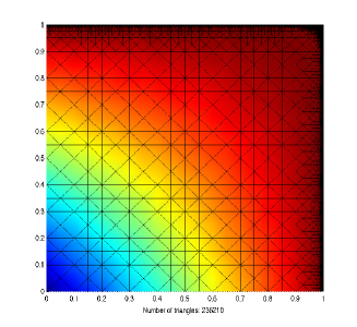
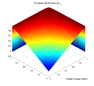
Figure 1. Adaptively refined mesh (left) and 3D plot of the corresponding approximate solution $u_{h}$ (right) by HDG-P2 for the case $\epsilon=10^{-4}$.

Example 6.1.

We consider a boundary layer problem in [4]. The convection-diffusion equation (1.1) is solved in the domain $\Omega=[0,1]\times[0,1]$ with $\beta=[1,1]^{T}$, $c=0$. The source term $f$ and the Dirichlet boundary condition are chosen such that

$$u(x,y)=x+y(1-x)+\frac{e^{-1/\epsilon}-e^{-(1-x)(1-y)/\epsilon}}{1-e^{-1/\epsilon}}$$

is the exact solution.

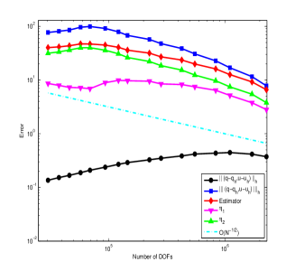
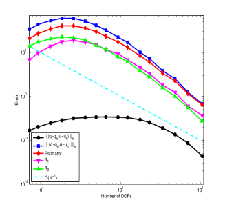
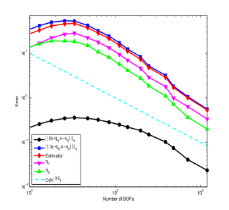
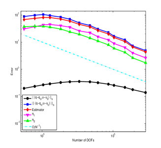
Figure 2. Convergence history of the adaptive HDG method. Left-Right: $\epsilon=10^{-5},\epsilon=10^{-6}$. Top-Bottom: $P1$-$P3$.

The solution develops boundary layers along the boundaries $x=1$ and $y=1$ for small $\epsilon$. The initial quasi-uniform mesh consists of 800 triangles and the initial mesh size $h_{0}=0.05$. Actually, our algorithm is robust for any coarser mesh. Figure 1 displays the adaptively refined mesh and the corresponding approximate solution $u_{h}$ by 20 iterations of the adaptive HDG-P2 method for two cases $\epsilon=10^{-4}$ and $\epsilon=10^{-5}$. One can observe that the mesh is always locally refined at the singularities along the boundaries $x=1$ and $y=1$, and the boundary layer solution can be captured on the adaptively refined mesh. In Figure 2, we show the error $\|({\boldsymbol{q}}-{\boldsymbol{q}}_{h},u-u_{h})\|_{h}$, the total energy error $\interleave({\boldsymbol{q}}-{\boldsymbol{q}}_{h},u-u_{h})\interleave_{h}$ (the total energy error is defined in (2.9)), the a posteriori error estimators $\eta_{1}$ and $\eta_{2}$, and the total a posteriori error estimator as functions of $N$ which is the number of degrees of freedom (DOFs) of $\widehat{u}_{h}$ for two cases $\epsilon=10^{-5}$ and $\epsilon=10^{-6}$ by HDG-P1, HDG-P2 and HDG-P3 respectively. In the following, we always let DOFs refer to the DOFs of $\widehat{u}_{h}$. For the case $\epsilon=10^{-5}$, the convergence results indicate the robustness of the proposed a posteriori error estimator and the almost optimal convergence rate $O(N^{-p/2})$ for the adaptive HDG method when the number of DOFs is sufficiently large. Here, $p$ is the polynomial order. The convergence of $\eta_{1}$ and $\eta_{2}$ is similar as the total a posteriori error estimator. For smaller $\epsilon=10^{-6}$ in this example, although the convergence of the error $\|({\boldsymbol{q}}-{\boldsymbol{q}}_{h},u-u_{h})\|_{h}$ slows down, the convergence of the a posteriori error estimators and the total energy error is also almost $O(N^{-p/2})$ when $p=1,2$ and $O(N^{-1})$ when $p=3$ on the currently obtained meshes.

Example 6.2.

We consider an internal layer problem in [50]. We set $\Omega=[0,1]\times[0,1],\beta=[0,1]^{T},c=1$. The source term $f$ and the Dirichlet boundary condition are chosen such that

$$u(x,y)=0.5\left(1-{\rm tanh}\left(\frac{0.5-x}{\alpha}\right)\right)$$

is the exact solution, where $\alpha$ is the width of the internal layer.

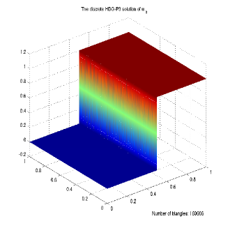
Figure 3. Adaptively refined mesh (Left) and 3D plot (Right) of the corresponding approximate solution $u_{h}$ by HDG-P3 for the case $\alpha=10^{-4}$ and $\epsilon=10^{-6}$.

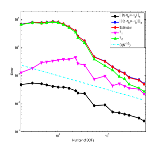
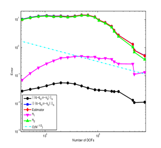
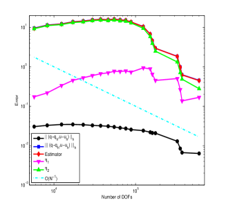
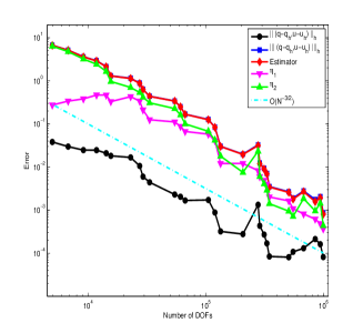
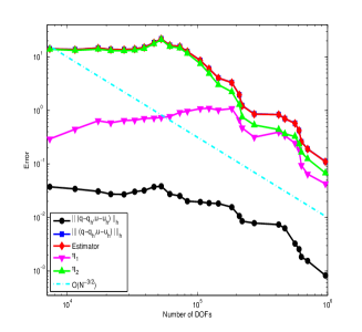
Figure 4. Convergence history of the adaptive HDG method. Left: $\alpha=10^{-3}$ and $\epsilon=10^{-5}$. Right: $\alpha=10^{-4}$ and $\epsilon=10^{-6}$. Top-Bottom: $P1$-$P3$.

The solution of this problem possesses an internal layer along $x=0.5$. The initial quasi-uniform mesh consists of 128 triangles and the initial mesh size $h_{0}=0.12$. The graphs of Figure 3 show the plots of the mesh and solution by 32 iterations of the adaptive HDG-P3 method for the case $\alpha=10^{-4}$ and $\epsilon=10^{-6}$. We can see that the singularities of the solutions can also be captured near $x=0.5$ on the adaptively refined mesh. Figure 4 shows the convergence of the corresponding errors. The robustness of the proposed a posteriori error estimator and the almost optimal convergence rate of the adaptive HDG method can be observed for HDG-P1, HDG-P2 and HDG-P3 when the number of DOFs is large enough. Moreover, we can also see that $\eta_{1}$ and $\eta_{2}$ converge similarly as the total a posteriori error estimator.

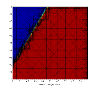
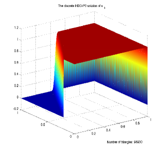
Figure 5. Adaptively refined mesh (Left) and the 3D plot (Right) of the corresponding approximate solution $u_{h}$ by HDG-P3 for the case $\epsilon=10^{-4}$.

Example 6.3.

This example is also taken from [4]. We set $\beta=[1/2,\sqrt{3}/2]^{T},c=0$, the source term $f=0$ and the Dirichlet boundary conditions as follows:

$$u=\begin{cases}1&\text{on $\{y=0,0\leq x\leq 1\}$ },\\ 1&\text{on $\{x=0,0\leq y\leq 1/5\}$ },\\ 0&\text{elsewhere }.\end{cases}$$

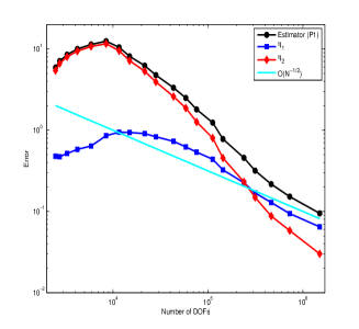
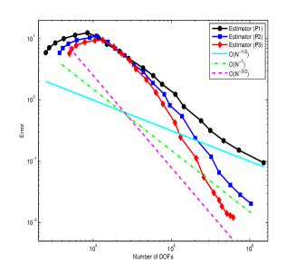
Figure 6. Convergence history of $\eta_{1}$, $\eta_{2}$ and the total a posteriori error estimator $\eta$ by HDG-P1 (Left) and comparing of convergence history of the estimator by HDG-P1, HDG-P2 and HDG-P3 (Right) for the case $\epsilon=10^{-4}$.

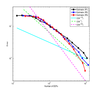
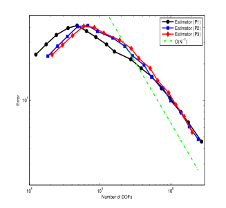
Figure 7. Convergence history of the estimator $\eta$ by HDG-P1, HDG-P2 and HDG-P3. Left: $\epsilon=10^{-5}$. Right: $\epsilon=10^{-6}$.

The solution of this problem possesses both interior layer and outflow layer. The initial quasi-uniform mesh consists of 800 triangles and the initial mesh size $h_{0}=0.05$. The graphs of Figure 5 show the adaptively refined mesh and the 3D plot of the corresponding approximate solution $u_{h}$ by 23 iterations of the adaptive HDG-P3 method for the case $\epsilon=10^{-4}$. Figure 5 indicates that both the interior and outflow layers can be captured by the adaptively refined mesh strategy. In particular, when the mesh size is $O(\epsilon)$ near the outflow layer and $O(\sqrt{\epsilon})$ near the interior layer, both interior and outflow layers can be captured well. Since there is no exact solution for this problem, we only show the convergence of the proposed a posteriori error estimator for the cases $\epsilon=10^{-4},10^{-5}$ and $10^{-6}$ in Figure 6 and Figure 7. For the cases $\epsilon=10^{-4},10^{-5}$, the almost optimal convergence rate $O(N^{-p/2})$ of the estimator can be observed for HDG-P1, HDG-P2 and HDG-P3 when the number of DOFs is large enough, and the convergence rate is faster when $p$ is larger. From the left graph of Figure 6, we can also see that $\eta_{1}$ and $\eta_{2}$ converge similarly as the total a posteriori error estimator for the case $\epsilon=10^{-4}$ by HDG-P1. Actually, for other cases the convergence property of $\eta_{1}$ and $\eta_{2}$ is always similar. For smaller $\epsilon=10^{-6}$, the convergence of the total a posteriori error estimator is almost the same as $O(N^{-1})$ for $p=1,2,3$ on the currently obtained meshes.

Appendix A. Estimate of $I_{1}$

By the Cauchy-Schwarz and Young’s inequalities, we get, for any $\delta>0$,

$$I_{1} \leq\frac{\delta}{2}\epsilon^{-1}\|{\boldsymbol{q}}-{\boldsymbol{q}}_{h}\|^{2}_{0,{\mathcal{T}}_{h}}+\frac{1}{2\delta}\|\nabla\psi e^{-\psi}\|^{2}_{L^{\infty}(\Omega)}\epsilon\|u_{h}-u^{{\mathcal{I}}}_{h}\|^{2}_{0,{\mathcal{T}}_{h}}$$ (A.1)

$$\quad+\frac{\delta}{2}\epsilon^{-1}\|{\boldsymbol{q}}-{\boldsymbol{q}}_{h}\|^{2}_{0,{\mathcal{T}}_{h}}+\frac{1}{2\delta}\|\varphi\|^{2}_{L^{\infty}(\Omega)}\epsilon^{-1}\|{\boldsymbol{q}}_{h}+\epsilon\nabla u^{{\mathcal{I}}}_{h}\|^{2}_{0,{\mathcal{T}}_{h}}$$

$$\leq\delta\epsilon^{-1}\|{\boldsymbol{q}}-{\boldsymbol{q}}_{h}\|^{2}_{0,{\mathcal{T}}_{h}}+\frac{1}{2\delta}\|\nabla\psi e^{-\psi}\|^{2}_{L^{\infty}(\Omega)}\epsilon\|u_{h}-u^{{\mathcal{I}}}_{h}\|^{2}_{0,{\mathcal{T}}_{h}}$$

$$\quad+\frac{1}{\delta}\|\varphi\|^{2}_{L^{\infty}(\Omega)}\left(\epsilon^{-1}\|{\boldsymbol{q}}_{h}+\epsilon\nabla u_{h}\|^{2}_{0,{\mathcal{T}}_{h}}+\epsilon\|\nabla u_{h}-\nabla u^{{\mathcal{I}}}_{h}\|^{2}_{0,{\mathcal{T}}_{h}}\right).$$

Appendix B. estimate of $I_{4}$

Now we consider the estimate of $I_{4}$. It is clear that

$$-\left({\boldsymbol{\beta}}\cdot\nabla(u-u^{{\mathcal{I}}}_{h}),\varphi(u-u^{{\mathcal{I}}}_{h})\right)_{{\mathcal{T}}_{h}}=\frac{1}{2}\left({\boldsymbol{\beta}}\cdot\nabla\varphi,(u-u^{{\mathcal{I}}}_{h})^{2}\right)_{{\mathcal{T}}_{h}}+\frac{1}{2}\left({\rm div}{\boldsymbol{\beta}}\,,\varphi(u-u^{{\mathcal{I}}}_{h})^{2}\right)_{{\mathcal{T}}_{h}},$$

which can be obtained by integration by parts and $\langle{\boldsymbol{\beta}}\cdot{\boldsymbol{n}},\varphi(u-u^{{\mathcal{I}}}_{h})^{2}\rangle_{\partial{\mathcal{T}}_{h}}=0$. Then, we have

$$I_{4} =\left({\boldsymbol{\beta}}\cdot\nabla\varphi(u-u_{h}),u_{h}-u^{{\mathcal{I}}}_{h}\right)_{{\mathcal{T}}_{h}}+\frac{1}{2}\left({\boldsymbol{\beta}}\cdot\nabla\varphi(u^{{\mathcal{I}}}_{h}-u_{h}),u^{{\mathcal{I}}}_{h}-u_{h}\right)_{{\mathcal{T}}_{h}}$$

$$\quad+2\big{(}(c-\frac{1}{2}{\rm div}{\boldsymbol{\beta}})(u^{{\mathcal{I}}}_{h}-u_{h}),\varphi(u-u_{h})\big{)}_{{\mathcal{T}}_{h}}-\big{(}(c-\frac{1}{2}{\rm div}{\boldsymbol{\beta}})(u^{{\mathcal{I}}}_{h}-u_{h}),\varphi(u^{{\mathcal{I}}}_{h}-u_{h})\big{)}_{{\mathcal{T}}_{h}}.$$

Appling the Cauchy-Schwarz and Young’s inequalities, we get

$$I_{4}\leq\frac{1}{2}(C^{d}_{5}+2C^{d}_{6})(\frac{1}{\delta}+1)\|u_{h}-u^{{\mathcal{I}}}_{h}\|^{2}_{0,{\mathcal{T}}_{h}}+(\frac{1}{2}C^{d}_{5}+C^{d}_{6})\delta\|u-u_{h}\|^{2}_{0,{\mathcal{T}}_{h}},$$ (B.1)

where $C^{d}_{5}=\|{\boldsymbol{\beta}}\cdot\nabla\varphi\|_{L^{\infty}(\Omega)},C^{d}_{6}=\|\varphi(c-\frac{1}{2}{\rm div}{\boldsymbol{\beta}})\|_{L^{\infty}(\Omega)}$.

Appendix C. Proof of Lemma 5.1

Proof.

We begin by the estimate $\alpha^{2}_{T}\|R_{h}\|^{2}_{0,T}\leq 2\alpha^{2}_{T}\|P_{W}R_{h}\|^{2}_{0,T}+2osc^{2}_{h}(R_{h},T)$. Note that for any $w\in H^{1}_{0}(T)$, we have

$$(R_{h},w)_{T}=({\rm div}({\boldsymbol{q}}-{\boldsymbol{q}}_{h})+{\boldsymbol{\beta}}\cdot\nabla(u-u_{h}),w)_{T}+(c(u-u_{h}),w)_{T}.$$

Moreover, for the element bubble function $B_{T}$, we have

$$\|P_{W}R_{h}\|^{2}_{0,T}\thickapprox\int_{T}B_{T}(P_{W}R_{h})^{2}\thickapprox\|B_{T}P_{W}R_{h}\|^{2}_{0,T}.$$

Here, we use $A\thickapprox B$ if $CB\leq A\leq CB$ with positive constant $C$. Taking $w=B_{T}P_{W}R_{h}$, we derive that

$$\|P_{W}R_{h}\|^{2}_{0,T} \thickapprox(P_{W}R_{h},w)_{T}=(R_{h},w)_{T}-(R_{h}-P_{W}R_{h},w)_{T}$$

$$=({\rm div}({\boldsymbol{q}}-{\boldsymbol{q}}_{h})+{\boldsymbol{\beta}}\cdot\nabla(u-u_{h}),w)_{T}+(c(u-u_{h}),w)_{T}-(R_{h}-P_{W}R_{h},w)_{T}.$$

Then, we can conclude the proof is complete by the above estimates and the Young’s inequality. ∎

References

- [1] R. Adams, Sobolev Spaces, Academic Press, New York, 1975.
- [2] M. Ainsworth and J. Oden, A Posteriori Error Estimation in Finite Element Analysis, Wiley-Interscience Series in Pure and Applied Mathematics, New York: Wiley, 2000.
- [3] L.E. Alaoui, A. Ern, and E. Burman, A priori and a posteriori analysis of nonconforming finite elements with face penalty for advection-diffusion equations, IMA J. Numer. Anal., 27 (2007) , pp. 151–171.
- [4] B. Ayuso and D. Marini, Discontinuous Galerkin methods for advection-diffusion-reaction problems, SIAM J. Numer. Anal., 47 (2009), pp. 1391–1420.
- [5] S. Badia and R. Codina, Analysis of a stabilized finite element approximation of the transient convection-diffusion equation using an ALE framework, SIAM J. Numer. Anal., 44 (2006), pp. 2159–2197.
- [6] A. N. Brooks and T.J.R. Hughes, Streamline upwind/Petrov-Galerkin formulations for convection dominated flows with particular emphasis on the incompressible Navier-Stokes equations, Comput. Methods Appl. Mech. Engrg., 32 (1982), pp.199–259.
- [7] F. Brezzi, T.J.R. Hughes, L.D. Marini, A. Russo, and E. Süli, A priori error analysis of residual-free bubbles for advection-diffusion problems, SIAM J. Numer. Anal., 36 (1999), pp. 1933–1948.
- [8] F. Brezzi, L.D. Marini, and E. Süli, Residual-free bubbles for advection-diffusion problems: the general error analysis, Numer. Math., 85 (2000), pp. 31–47.
- [9] D. Broersen and R. Stevenson, A Petrov-Galerkin discretization with optimal test space of a mild-weak formulation of convection-diffusion equations in mixed form, IMA J. Numer. Anal., 2014, accepted.
- [10] Erik Burman and Alexandre Ern, Stabilized Galerkin approximation of convection-diffusion-reaction equations: discrete maximum principle and convergence, Math. Comp., 74 (2005), pp. 1637–1652.
- [11] E. Burman and P. Hansbo, Edge stabilization for Galerkin approximations of convection-diffusion-reaction problems, Comput. Methods Appl. Mech. Engrg., 193 (2004), pp. 1437–1453.
- [12] E. Burman and A. Ern, Continuous interior penalty -finite element methods for advection and advection-diffusion equations, Math. Comp., 76 (2007), pp. 1119–1140.
- [13] J. Chan, N. Heuer, T. Bui-Thanh, and L. Demkowicz, A robust DPG method for convection-dominated diffusion problems II: Adjoint boundary conditions and mesh-dependent test norms, Computers & Mathematics with Applications, 67 (2014), pp. 771–795.
- [14] Y. Chen and B. Cockburn, Analysis of variable-degree HDG methods for convection-diffusion equations. Part I: General nonconforming meshes, IMA J. Num. Anal., 32(4) (2012), 1267–1293.
- [15] H. Chen, G. Fu, J. Li, and W. Qiu, First order least square method with ultra-weakly imposed boundary condition for convection dominated diffusion problems, submitted, arXiv:1309.7108[math.NA] (2013).
- [16] R. Codina and J. Blasco, Analysis of a stabilized finite element approximation of the transient convection-diffusion-reaction equation using orthogonal subscales, Comput. Vis. Sci., 4 (2002), pp. 167–174.
- [17] B. Cockburn, B. Dong, J. Guzmán, M. Restelli, and R. Sacco, A hybridizable discontinuous Galerkin method for steady-state convection-diffusion-reaction problems, J. Sci. Comput., 31 (2009), pp. 3827–3846.
- [18] B. Cockburn, J. Gopalakrishnan, and R. Lazarov, Unified hybridization of discontinuous Galerkin, mixed, and continuous Galerkin methods for second order elliptic problems, SIAM J. Numer. Anal., 47 (2009), pp. 1319–1365 .
- [19] B. Cockburn, J. Gopalakrishnan, and F.J. Sayas, A projection-based error analysis of HDG methods, Math Comp., 79 (2010), pp. 1351–1367.
- [20] B. Cockburn and W. Zhang, A posteriori error estimates for HDG methods, J. Sci. Comput., 51 (2012), pp. 582–607.
- [21] B. Cockburn and W. Zhang, A posteriori error analysis for hybridizable discontinuous Galerkin methods for second order elliptic problems, SIAM J. Numer. Anal., 51 (2013), pp. 676–693.
- [22] B. Cockburn and W. Zhang, An a posteriori error estimate for the variable-degree Raviart-Thomas method, Math. Comp., 83 (2014), pp. 1063–1082.
- [23] L. Demkowicz and N. Heuer, Robust DPG method for convection-dominated diffusion problems, SIAM J. Numer. Anal., 51 (2013), pp. 2514–2537.
- [24] W. Eckhaus, Boundary layers in linear elliptic singular perturbation problems, SIAM Rev., 14 (1972), pp. 225–270.
- [25] H. Egger and J. Schöberl, A hybrid mixed discontinuous Galerkin finite-element method for convection–diffusion problems, IMA J. Num. Anal., 30 (2010), 1206–1234.
- [26] K. Eriksson and C. Johnson, Adaptive streamline diffusion finite element methods for stationary convection-diffusion problems, Math. Comp., 60 (1993), pp. 167–188.
- [27] A. Ern and A. Stephansen, A posteriori energy-norm error estimates for advection-diffusion equations approximated by weighted interior penalty methods, J. Comput. Math., 26 (2008), pp. 488–510.
- [28] A. Ern, A. Stephansen, and M.Vohralík, Guaranteed and robust discontinuous Galerkin a posteriori error estimates for convection-diffusion-reaction problems, J. comput. Appl. Math., 234 (2010), pp. 114–130.
- [29] H. Goering, A. Felgenhauer, G. Lube, H.-G. Roos, and L. Tobiska, Singularly Perturbed Differential Equations, Akademie-Verlag, Berlin, 1983.
- [30] J. Guzmán, Local analysis of discontinuous Galerkin methods applied to singularly perturbed problems, J. Numer. Math.,14 (2006), pp. 41–56.
- [31] G. Fu, W. Qiu and W. Zhang, An analysis of HDG methods for convection-dominated diffusion problems, submitted, arXiv:1310.0887[math.NA] (2013).
- [32] P. Houston, C. Schwab and E. Süli, Discontinuous hp-finite element methods for advection-diffusion-reaction problems, SIAM J. Num. Anal., 39 (2002), pp. 2133–2163.
- [33] T.J.R. Hughes, G. Scovazzi, P. Bochev, and A. Buffa, A multiscale discontinuous Galerkin method with the computational structure of a continuous Galerkin method, Comput. Methods Appl. Mech. Engrg., 195 (2006), pp. 2761–2787.
- [34] O. A. Karakashian and F. Pascal, A posteriori error estimates for a discontinuous Galerkin approximation of a second order elliptic problems, SIAM J. Numer. Anal., 41 (2003), pp. 2374–2399.
- [35] O. A. Karakashian and F. Pascal, Convergence of adaptive discontinuous Galerkin approximations of second-order elliptic problems, SIAM J. Numer. Anal., 45 (2007), pp. 641–665.
- [36] R.M. Kirby, S.J. Sherwin, and B. Cockburn, To CG or to HDG: A comparative study, J. Sci. Comput., 51 (2012), pp. 183–212.
- [37] P. Knobloch and L. Tobiska, On the stability of finite element discretizations of convection diffusion reaction equations, IMA J. Numer. Anal., 31 (2011), pp. 147–164.
- [38] N.C. Nguyen, J. Peraire, and B. Cockburn, An implicit high-order hybridizable discontinuous Galerkin method for linear convection-diffusion equations, J. Comput. Phys., 288 (2009), pp. 3232–3254.
- [39] W. Reed and T. Hill, Triangular mesh methods for the neutron transport equation, Technical Report LA- UR-73-479, Los Alamos Scientific Laboratory, 1973.
- [40] H.-G. Roos, M. Stynes, and L. Tobiska, Robust Numerical Methods for Singularly Perturbed Differential Equations, volume 24 of Springer Series in Computational Mathematics, Springer-Verlag, Berlin, 2008, Second edition.
- [41] G. Sangalli, Robust a posteriori estimator for advection-diffusion-reaction problems, Math. Comp., 77 (2008), pp. 41–70.
- [42] D. Schötzau and L. Zhu, A robust a posteriori error estimator for discontinuous Galerkin methods for convection diffusion equations, Appl. Numer. Math., 59 (2009), pp. 2236–2255.
- [43] R. Stevenson, Optimality of a standard adaptive finite element method, Foundations of Computional Mathematics, 2 (2007), pp. 245–269.
- [44] M. Stynes, Steady state convection diffusion problems, Acta Numer., 14 (2005), pp. 445–508.
- [45] L. Tobiska and R. Verfürth, Robust a posteriori error estimates for stabilized finite element methods, submitted, arXiv:1402.5892[math.NA], (2014).
- [46] U. Nävert, A finite element method for convection-diffusion problems. PhD thesis, Department of Computer Science, Chalmers University of Technology, Göteborg, 1982.
- [47] R.Verfürth, A Review of Posteriori Error Estimation and Adaptive Mesh-refinement Techniques, Wiley-Teubner, Chichester,1996.
- [48] R.Verfürth, A posteriori error estimators for convection-diffusion equations, Numer. Math., 80 (1998), pp. 641–663.
- [49] R.Verfürth, Robust a posteriori error estimates for stationary convection-diffusion equations, SIAM J.Numer. Anal., 43 (2005), pp. 1766–1782.
- [50] M.Vohralík, A posteriori error estimates for lowest-order mixed finite element discretizations of convection-diffusion-reaction equations, SIAM J. Numer. Anal., 45 (2007), pp.1570–1599.
- [51] M.Vohralík, Residual flux-based a posteriori error estimates for finite volume and related locally conservative methods, Numer. Math., 111 (2008), pp. 121–158.
- [52] L. Zhu and D. Schötzau, A robust a posteriori error estimate for hp-adaptive DG methods for convection-diffusion equations, IMA J. Numer. Anal., 31 (2011), pp. 971–1005.
- [53] L. Zhu, S. Giani, P. Houston, and D. Schötzau, Energy norm a posteriori error estimation for hp-adaptive discontinuous Galerkin methods for elliptic problems in three dimensions, Math. Models Methods Appl. Sci., 21 (2011), pp. 267–306.