Historical Backtesting of Local Volatility Model using AUD/USD Vanilla Options

Abstract

The Local Volatility model is a well-known extension of the Black-Scholes constant volatility model whereby the volatility is dependent on both time and the underlying asset. This model can be calibrated to provide a perfect fit to a wide range of implied volatility surfaces. The model is easy to calibrate and still very popular in FX option trading. In this paper we address a question of validation of the Local Volatility model. Different stochastic models for the underlying can be calibrated to provide a good fit to the current market data but should be recalibrated every trading date. A good fit to the current market data does not imply that the model is appropriate and historical backtesting should be performed for validation purposes. We study delta hedging errors under the Local Volatility model using historical data from 2005 to 2011 for the AUD/USD implied volatility. We performed backtests for a range of option maturities and strikes using sticky delta and theoretically correct delta hedging. The results show that delta hedging errors under the standard Black-Scholes model are no worse than that of the Local Volatility model. Moreover, for the case of in and at the money options, the hedging error for the Back-Scholes model is significantly better.

1 Introduction

Under the well-known Black-Scholes pricing model [1], the asset price $S$ is modelled with geometric Brownian motion,

$$dS_{t}=\mu_{t}S_{t}dt+\sigma S_{t}dW_{t}\ ,$$ (1)

where $\mu_{t}$ is the drift, $\sigma$ is volatility and $W_{t}$ is a standard Brownian motion. One of the key assumptions of the model is the no-arbitrage condition, which means that it is impossible to make a riskless profit. From this assumption it can be shown that the fair price of a derivative security with underlying asset $S$ is equal to the mathematical expectation of the discounted payoff of the derivative. This expectation is computed with respect to a so-called risk-neutral probability measure. Furthermore, under this measure the dynamics of the asset price $S$ is given by

$$dS_{t}=(r-q)S_{t}dt+\sigma S_{t}dB_{t},$$ (2)

where $B_{t}$ is a standard Brownian motion under the risk neutral measure, $r$ is the constant risk-free interest rate and $q$ denotes the constant dividend yield. Given the price of an European option, strike, maturity and interest rates, the asset price volatility $\sigma$ can be computed numerically from the Black-Scholes pricing formula. We say that $\sigma$ is the volatility implied by the market price. If the Black-Scholes model was a perfect representation of the market, then the implied volatility would be equal for all market traded options. This is definitely not the case in practice.

The implied volatility is heavily dependent on the strike price and maturity of the option. The local volatility model is an extension of the Black-Scholes framework which can account for this dependence, and it does so by making volatility a function of the current time and current spot price i.e. $\sigma(S_{t},t)$. (2) is then replaced by

$$dS_{t}=(r-q)S_{t}dt+\sigma(S_{t},t)S_{t}dW_{t}.$$ (3)

2 The Black-Scholes setup

Let $V(S,t)$ denote the discounted price of a contingent claim at time $t$ with underlying asset price $S(t)$. Let $r$ denote the risk-free interest rate, $q$ denote the dividend yield and $\sigma$ the asset price volatility. Within the Black-Scholes framework, $V$ satisfies the fundamental partial differential equation (PDE)

$$\frac{\partial V}{\partial t}+\frac{1}{2}\sigma^{2}S^{2}\frac{\partial^{2}V}{\partial S^{2}}+(r-q)S\frac{\partial V}{\partial S}-rV=0,$$ (4)

with known boundary condition $V(S(T),T)$ for the case of European options. This PDE can be obtained by applying a trading strategy called delta hedging.

For ease of numerical implementation we transform the above PDE with $X=\log S$. Routine calculations show that the transformed PDE is

$$\frac{\partial V}{\partial t}+(r-q-\frac{1}{2}\sigma^{2})\frac{\partial V}{\partial X}+\frac{\sigma^{2}}{2}\frac{\partial^{2}V}{\partial X^{2}}-rV=0.$$ (5)

2.1 The Black-Scholes pricing formula

Assuming constant interest rates $r_{c}$, dividend yields $q_{c}$ and volatility $\sigma_{c}$, the Black-Scholes formula for the price of an European call option with strike $K$ and maturity $T$, at zero time $t=0$, is given by

$$C (\sigma_{c},K,T,r_{c},q_{c},S_{0})$$

$$=e^{-r_{c}T}\left(S_{0}e^{(r_{c}-q_{c})T}\Phi(d_{1})-K\Phi(d_{1}-\sigma_{c}\sqrt{T})\right),$$ (6)

where $\Phi(\cdot)$ denotes the cumulative distribution function for standard Normal distribution and

$$d_{1}=\frac{\ln\left(\frac{S_{0}}{K}\right)+\left(r_{c}-q_{c}+\frac{1}{2}\sigma_{c}^{2}\right)T}{\sigma_{c}\sqrt{T}}.$$

For the case where interest rates, dividend yields and volatility are time-dependent, the Black-Scholes formula can be applied with the following substitutions ([2, sec. 8.8] )

$$r_{c} =\frac{1}{T}\int_{0}^{T}r(u)du,$$ (7)

$$q_{c} =\frac{1}{T}\int_{0}^{T}q(u)du,$$ (8)

$$\sigma^{2}_{c} =\frac{1}{T}\int_{0}^{T}\sigma^{2}(u)du,$$ (9)

where $r(t)$, $q(t)$ and $\sigma(t)$ are called the instantaneous interest rate, instantaneous dividend yield and instantaneous volatility respectively. The interpretation is that in a small interval of time $[t,t+\Delta t]$, the amount of interest accrued/owed is $r(t)\Delta t$. Note that $r(t)$, $q(t)$ and $\sigma(t)$ are not observable in the market but instead we observe the integrals in (7), (8) and (9); see sections 5.3 and 5.4 for more discussion on this point and for how to input the correct values from market data.

3 Local volatility

The local volatility model extends the Black-Scholes framework by making volatility a function of current asset price and time. In addition we introduce time dependence for the interest rate and dividend yield. This leads to the following modification of equation (5),

$$\frac{\partial V}{\partial t} +(r(t)-q(t)-\frac{1}{2}[\sigma(e^{X_{t}},t)]^{2})\frac{\partial V}{\partial X}$$

$$+\frac{1}{2}[\sigma(e^{X_{t}},t)]^{2}\frac{\partial^{2}V}{\partial X^{2}}-r(t)V=0,$$ (10)

where the local volatility $\sigma(K,T)$ is given by

$$\sigma (K,T)$$

$$=\sqrt{\frac{2\theta T\frac{\partial\theta}{\partial T}+2(r(T)-q(T))K\theta T\frac{\partial\theta}{\partial K}}{\left[1+d_{1}K\sqrt{T}\frac{\partial\theta}{\partial K}\right]^{2}+K^{2}\theta T\left[\frac{\partial^{2}\theta}{\partial K^{2}}-d_{1}\left(\frac{\partial\theta}{\partial K}\right)^{2}\sqrt{T}\right]}},$$ (11)

$$d_{1} =\frac{\ln\left(\frac{S_{0}}{K}\right)+\int_{0}^{T}[r(t)-q(t)]dt+\frac{1}{2}\theta^{2}T}{\theta\sqrt{T}}.$$ (12)

Here we define $\theta(K,T)=C^{-1}(V)$, where $V=C(\theta,\cdot)$ is given by the Black-Scholes formula (2.1). That is, $\theta$ is the market implied volatility for a vanilla option with strike $K$ and maturity $T$. Equation (11) is sometimes called the Dupire formula. For a proof of the formula, see [3, p. 49].

The functions $r(t)$ and $q(t)$ are the instantaneous rates; see section 5.3 on how to determine these functions from market data.

To compute local volatility we require an implied volatility surface that can be interpolated from market data. There is no universal way to perform this interpolation. We now describe a simple method that yields good results for FX data.

3.1 Interpolating market implied volatility

To compute the local volatility function (11), we need partial derivatives of the implied volatility surface $\theta(K,T)$. In practice we only have a finite number of market data points, typically $5$ values for a given maturity and about $10$ maturities; see table 1. We need some interpolating procedure for $\theta$. This is an ill-posed problem, and there are a number of ways to interpolate these data points. We use natural cubic splines to interpolate across strikes and maturities.

Maturity / $\Delta$	$\boldsymbol{10\Delta}$Put	$\boldsymbol{25\Delta}$Put	ATM	$\boldsymbol{25\Delta}$Call	$\boldsymbol{10\Delta}$Call
1 week	9.963%	9.088%	8.450%	8.213%	8.338%
1 month	10.913%	10.038%	9.400%	9.163%	9.288%
2 months	11.363%	10.488%	9.850%	9.613%	9.738%
3 months	11.713%	10.838%	10.200%	9.963%	10.138%
6 months	12.155%	11.280%	10.630%	10.430%	10.605%
1 year	12.400%	11.525%	10.850%	10.675%	10.850%
2 years	12.157%	11.350%	10.750%	10.650%	10.844%
3 years	12.013%	11.250%	10.700%	10.650%	10.888%
4 years	11.966%	11.225%	10.700%	10.675%	10.935%
5 years	11.819%	11.100%	10.600%	10.600%	10.881%

Table 1: An example of AUD/USD market implied volatilities on 12 April 2005. The spot price for that day was $S_{0}=0.7735$.

3.2 Our method to compute local volatility

Suppose we have market data for $N$ different maturities and that for each maturity $M$ options are available. Let $K^{(i)}_{j}$ and $\theta^{(i)}_{j}$ denote the strike and implied volatility of the j-th vanilla option with maturity $T_{i}$.

1. Interpolation across strikes: For each market maturity $T_{i}$, $i\in\left\{1,\dots,N\right\}$ fit a natural cubic spline $y_{i}(k)$ through

   $$\left(K^{(i)}_{1},\theta^{(i)}_{1}\right),\left(K^{(i)}_{2},\theta^{(i)}_{2}\right),\dots,\left(K^{(i)}_{M},\theta^{(i)}_{M}\right).$$

   Note that $y_{i}^{\prime}(K)=\frac{\partial\theta}{\partial K}_{|(K,T_{i})}$ and $y_{i}^{\prime\prime}(K)=\frac{\partial^{2}\theta}{\partial K^{2}}_{|(K,T_{i})}$.

2. Interpolation across maturities: To find $\frac{\partial\theta}{\partial K}$ at any given $(K,T)$ fit another natural cubic spline $z(t)$ through

   $$\left(T_{1},y_{1}^{\prime}(K)\right),\left(T_{2},y_{2}^{\prime}(K)\right),\dots,\left(T_{N},y_{N}^{\prime}(K)\right).$$

   Then $\frac{\partial\theta}{\partial K}=z(T)$.

3. Similarly to find $\frac{\partial^{2}\theta}{\partial K^{2}}$ at any given $(K,T)$ fit another natural cubic spline $w(t)$ through

   $$\left(T_{1},y_{1}^{\prime\prime}(K)\right),\left(T_{2},y_{2}^{\prime\prime}(K)\right),\dots,\left(T_{N},y_{N}^{\prime\prime}(K)\right).$$

   Then $\frac{\partial^{2}\theta}{\partial K^{2}}=w(T)$.

4. To find $\theta$ and $\frac{\partial\theta}{\partial T}$ at $(K,T)$, fit a natural cubic spline $u(t)$ through

   $$\left(T_{1},y_{1}(K)\right),\left(T_{2},y_{2}(K)\right),\dots,\left(T_{N},y_{N}(K)\right).$$

   Then $\theta(K,T)=u(T)$ and $\frac{\partial\theta}{\partial T}=u^{\prime}(T)$.

5. Substitute above into (11) and compute $\left[\sigma(K,T)\right]^{2}$. If $\left[\sigma(K,T)\right]^{2}<0$ then we overwrite

   $$\sigma(K,T)=0.$$

Note that the method can obtain a value for local volatility for any $(K,T)$ pair beyond the market range (for $T$ smaller than the first market maturity, larger than the last market maturity etc), by linear extrapolation of the natural cubic splines. For example, if we have a natural cubic spline $y(x)$ fitted to data points $x_{1},x_{2},\dots,x_{n}$ then our extrapolation function $y^{*}(x)$ is defined by $y(x^{*})$ for $x*<x_{1}$ by

$$y^{*}(x)=\begin{cases}y^{\prime}(x_{1})(x-x_{1})+y(x_{1}),\textrm{ if $x<x_{1}$,}\\ y(x),\textrm{ if $x_{1}\leq x\leq x_{n}$,}\\ y^{\prime}(x_{n})(x-x_{n})+y(x_{n}),\textrm{ if $x>x_{n}$.}\end{cases}$$ (13)

4 Pricing using Crank-Nicolson method

Once we have a computable local volatility function, we can use the finite difference method to solve the PDE (10). Suppose that we would like to price an European call option with strike $K$ and maturity $T$ years. We approximate the PDE (10) with boundary conditions $V(S(T),T)=(S(T)-K)^{+}$.

4.1 Mesh properties

First we need a mesh of $(\textrm{price},\textrm{time})$ pairs. Suppose that we have $N$ different time points and $M$ different prices in the mesh. Furthermore, assume the mesh is rectangular and uniformly-spaced with boundaries of

• $0$ and $T$ for the time axis.

• $S_{0}\exp\left\{-D\right\}$ and $S_{0}\exp\left\{D\right\}$ for the price axis, where $D=\gamma\bar{\theta}\sqrt{T}$ and $\bar{\theta}$ is the average of the at the money implied volatilities. We set $\gamma=7$ which we determined experimentally as a value that resulted in an overall small numerical error for the Crank-Nicolson method. This value corresponds to a very small probability for the price to move beyond $S_{0}e^{D}$.

In addition, we scale the number of time points by $T$. Setting $N=500T+500$ gives sufficiently good results. Define $\Delta t=T/N$. Then the time interval $[0,T]$ is discretised by

$$t_{0}=0,t_{1}=\Delta t,t_{2}=2\Delta t,\dots,t_{N}=T.$$

Also define $\Delta x=2D/M$. Then the price interval $[S_{0}e^{-D},S_{0}e^{D}]$ is discretised by

$$s_{i}=S_{0}e^{-D+i(\Delta x)},$$

for $i=0,1,\dots,M$. This definition allows mesh points to coincide with the spot price. We did this for the convenience of the backtesting procedure to calculate difference vanillas using the same mesh. Next, the PDE (10) contains partial derivatives with respect to the logarithm of price. Let $x_{i}=\ln s_{i}$. Then

$$x_{i+1}-x_{i} =\ln s_{i+1}-\ln s_{i}$$

$$=\ln\left(\frac{S_{0}\exp\left\{-D+(i+1)\Delta x\right\}}{S_{0}\exp\left\{-D+i\Delta x\right\}}\right)$$

$$=\Delta x,$$

so the price points are indeed uniformly spaced in terms of log-prices.

4.2 The finite difference scheme

Let $i\in\left\{1,\dots,N\right\}$, $\nu(t,x)=r(t)-q(t)-\frac{1}{2}\left[\sigma(e^{x},t)\right]^{2}$ and $V_{j}^{i}=V(s_{j},t_{i})$. The Crank-Nicolson scheme is given by

$$a^{i-1}_{j}V_{j}^{i-1} -b^{i-1}_{j}V_{j+1}^{i-1}-c^{i-1}_{j}V_{j-1}^{i-1}$$

$$=d^{i}_{j}V_{j}^{i}+b^{i}_{j}V_{j+1}^{i}+c^{i}_{j}V_{j-1}^{i},$$ (14)

where

$$a^{i}_{j} =\frac{r(t_{i})}{2}+\frac{1}{\Delta t}+\frac{\sigma^{2}(t_{i},s_{j})}{2(\Delta x)^{2}},$$

$$b^{i}_{j} =\frac{\sigma^{2}(t_{i},s_{j})}{4(\Delta x)^{2}}+\frac{\nu(t_{i},s_{j})}{4\Delta x},$$

$$c^{i}_{j} =\frac{\sigma^{2}(t_{i},s_{j})}{4(\Delta x)^{2}}-\frac{\nu(t_{i},s_{j})}{4\Delta x},$$

$$d^{i}_{j} =\frac{1}{\Delta t}-\frac{r(t_{i})}{2}-\frac{\sigma^{2}(t_{i},s_{j})}{2(\Delta x)^{2}}.$$

For boundary conditions we use the fact that $\lim_{S\to 0}\frac{\partial V}{\partial S}=e_{0}$ and $\lim_{S\to\infty}\frac{\partial V}{\partial S}=e_{\infty}$ where

$$e_{0} =\begin{cases}0,\textrm{ if $V$ is price of call option}\\ -1,\textrm{ if $V$ is price of put option}\end{cases}$$

$$e_{\infty} =\begin{cases}1,\textrm{ if $V$ is price of call option}\\ 0,\textrm{ if $V$ is price of put option}\end{cases}$$

This leads to the following equations

$$V_{0}^{i}-V_{1}^{i} =e_{0}(s_{0}-s_{1}),$$ (15)

$$V_{M}^{i}-V_{M-1}^{i} =e_{\infty}(s_{M}-s_{M-1}).$$ (16)

To initiate the scheme, we set for all $j=\left\{0,\dots,M\right\}$

$$V_{j}^{N}=\begin{cases}\left(s_{j}-K\right)^{+},&\mbox{if we are pricing a call option.}\\ \left(K-s_{j}\right)^{+},&\mbox{if we are pricing a put option.}\end{cases}$$

We then repeatedly solve the system until we obtain $\left(V_{1}^{0},V_{2}^{0},\dots,V_{M}^{0}\right)^{\mathrm{T}}$ (for details see for e.g. [2]). If $M$ is an odd integer, the price of the option is $V_{(M+1)/2}^{0}$. Otherwise we may fit an interpolating function $\hat{V}(s)$ through

$$(s_{1},V^{0}_{1}),(s_{2},V^{0}_{2}),\dots,(s_{M},V^{0}_{M})$$

and the price is then $\hat{V}(S_{0})$. Also note that the delta of the option is $\hat{V}^{\prime}(S_{0})$. We have found that a natural cubic spline for $\hat{V}$ gives good results.

Remark: This pricing method is very fast if the meshpoints of our local volatility function coincide with the meshpoints in our finite difference scheme. This is how we implemented our scheme; we first set the mesh points for our finite difference scheme then pre-compute the local volatility function at these points.

5 Market data layout

In this paper we work with daily AUD/USD implied volatility data dating from 2005/03/22 to 2011/07/15. For each trading day, the market data contains a spot price and for a range of maturities (1 week, 1 month, 2 months, 3 months, 6 months, 1 year, 2 years, 3 years, 4 years and 5 years) there are

• implied volatility for at the money (ATM) options;

• risk reversals for 10 and 25 delta call, denoted by $RR_{10\Delta Call}$ and $RR_{25\Delta Call}$ respectively;

• butterflys for 10 and 25 delta put, denoted by $Fly_{10\Delta Put}$ and $Fly_{25\Delta Put}$ respectively;

• zero rates (yields) for the domestic and foreign currency.

From this data we need to extract the strike prices and implied volatilities for traded vanilla options. This is done through the Black-Scholes framework. Taking the Black-Scholes price of a call option (2.1) and differentiating, we obtain the call delta

$$\Delta_{call}(S_{0},K,T,\gamma_{d},\gamma_{f},\sigma) =\frac{\partial C(S_{0},K,T,\gamma_{d},\gamma_{f},\sigma)}{\partial S}$$

$$=e^{-\gamma_{f}T}\Phi(d_{1}),$$ (17)

where $\gamma_{d}=\frac{1}{T}\int_{0}^{T}f(t)dt$ and $\gamma_{f}=\frac{1}{T}\int_{0}^{T}q(t)dt$ denote the domestic and foreign yields respectively (this is discussed in detail in section 5.3). Utilising put-call parity the put delta is given by

$$\Delta_{put}(S_{0},K,T,\gamma_{d},\gamma_{f},\sigma)=\Delta_{call}(S_{0},K,T,\gamma_{d},\gamma_{f},\sigma)-e^{-\gamma_{f}T}.$$ (18)

Following a standard notation we use $10\Delta Put$ and $25\Delta Put$ to denote the volatility $\sigma$ and strike price $K$ that gives a put delta $\Delta_{put}$ of $10\%$ and $25\%$ respectively. Similarly, $10\Delta Call$ and $25\Delta Call$ denotes the volatility $\sigma$ and strike price $K$ that gives a call delta $\Delta_{call}$ of $10\%$ and $25\%$ respectively.

5.1 Computing implied volatilities

Using market definitions we reconstruct the market implied volatilities by using the following formulas,

$$\sigma_{10\Delta Put} =\sigma_{ATM}+Fly_{10\Delta}-\frac{1}{2}RR_{10\Delta},$$

$$\sigma_{25\Delta Put} =\sigma_{ATM}+Fly_{25\Delta}-\frac{1}{2}RR_{25\Delta},$$

$$\sigma_{25\Delta Call} =\sigma_{ATM}+Fly_{25\Delta}+\frac{1}{2}RR_{25\Delta},$$

$$\sigma_{10\Delta Call} =\sigma_{ATM}+Fly_{10\Delta}+\frac{1}{2}RR_{10\Delta}.$$

5.2 Computing strikes

After we determine the implied volatilities, the only parameter yet to be determined is the strike price. We use the delta formulas of (5) and (18) and an implementation of the inverse cumulative distribution function $\Phi^{-1}$ of the standard Normal distribution to determine the strike. For example, to obtain the strike price for the $10\Delta Put$ option we are looking for the value of $K$ satisfying

$$\delta_{put}(S_{0},K,T,\gamma_{d},\gamma_{f},\sigma_{10\Delta Put})=0.1,$$

which is easy to calculate via the inverse Normal distribution function.

5.3 Interest rates

On each trading day, we can extract from the market so called zero-coupon interest rates or zero rates for a range of different maturities. To explain the meaning of these rates we give an example. Suppose we have the following market zero rates for the Australian dollar:

Maturity (years)	Zero rate (%)
1	4.8
2	4.9
3	5
4	5.1

With continuous compounding of interest rates, a one year investment of $10 AUD grows to $10\times e^{0.048\times 1}=10.49$. Two year investment of the same amount grows to $10\times e^{0.049\times 2}=11.03$

We can now interpolate between these data points to obtain what is called a zero curve. There is no universally accepted way to perform this interpolation. Suppose the market rates are given by $(T_{1},\gamma_{1}),(T_{2},\gamma_{2}),\ldots,(T_{n},\gamma_{n})$ where $T_{i}$ denotes the $i^{th}$ maturity and $\gamma_{i}$ is its zero rate. We define our zero curve $\gamma(t)$ to be a function such that $t\gamma(t)$ is piecewise-linear through the points

$$(0,\gamma_{1}),(T_{1},\gamma_{1}),(T_{2},\gamma_{2}),\ldots,(T_{n},\gamma_{n}).$$

Now we will need to have the instantaneous interest rates for various calculations such as the Dupire formula (11). That is, we need to find the function $r(s)$ such that $\gamma(t)=\frac{1}{t}\int_{0}^{t}r(s)ds$. Since we assumed that $t\gamma(t)$ is piecewise-linear, it implies that $r(s)$ is piecewise-constant on the same intervals that $t\gamma(t)$ is piecewise-linear.

By construction $\gamma(t)=\gamma_{1}$ for $t\in[0,T_{1}]$ which implies that $r(t)=\gamma(t)$ over $[0,T_{1}]$. Next let $t\in(T_{i},T_{i+1}]$ and consider

$$\gamma(T_{i+1})T_{i+1}-\gamma(T_{i})T_{i} =\gamma_{i+1}T_{i+1}-\gamma_{i}T_{i}$$

$$=\int_{T_{i}}^{T_{i+1}}r(s)ds$$

$$=(T_{i+1}-T_{i})r(t),$$

so it follows that

$$r(t)=\frac{\gamma_{i+1}T_{i+1}-\gamma_{i}T_{i}}{T_{i+1}-T_{i}},\mbox{for $t\in(T_{i},T_{i+1}]$}.$$

In summary, the instantaneous interest rate is given by

$$r(t)=\begin{cases}\gamma_{1},\mbox{for $t\in[0,T_{1}]$}\\ \frac{\gamma_{i+1}T_{i+1}-\gamma_{i}T_{i}}{T_{i+1}-T_{i}},\mbox{for $t\in(T_{i},T_{i+1}]$, $i=1,\ldots,n-1$}\end{cases}$$ (19)

5.4 Term structure of volatility for Black-Scholes

To best compare performance of Black-Scholes with Local Volatility, we need to have time dependent volatilities for the Black-Scholes model. Under this condition, the market implied volatilities allow us to construct the term structure of volatility. Suppose that at the money implied volatilities are

$$(T_{1},\sigma_{1}),(T_{2},\sigma_{2}),\ldots,(T_{n},\sigma_{n})$$

Then similarly to the instantaneous interest rate of the previous section, we define the instantaneous volatility $\sigma:[0,T_{n}]\to R^{+}$ by

$$\sigma(t)=\begin{cases}\sigma_{1},\mbox{for $t\in[0,T_{1}]$}\\ \sqrt{\frac{\sigma^{2}_{i+1}T_{i+1}-\sigma^{2}_{i}T_{i}}{T_{i+1}-T_{i}}},\mbox{for $t\in(T_{i},T_{i+1}]$, $i=1,\ldots,n-1$}\end{cases}$$ (20)

From this define $\sigma_{avg}:[0,T_{n}]\to R^{+}$ by $\sigma_{avg}(t)=\sqrt{\frac{1}{t}\int_{0}^{t}\sigma^{2}(s)ds}$. Then it’s easy to check that $\sigma^{2}_{i}=\sigma^{2}_{avg}(T_{i})$ for all $i=1,\ldots,n$.

6 Calibrating the model

By calibrating the model, we mean a verification of our procedures above by comparing our results with market data. This is done by

1. Obtain current market data, and construct the local volatility surface as outlined in Section 3.2.

2. For each market traded option $V$,

   1. Obtain $V$’s strike price and maturity. Then apply the pricing methodology in Section 4 to obtain a price.

   2. Using the Black-Scholes formula (2.1), compute the implied volatility from the obtained price and compare with the market implied volatility of $V$. Ideally the computed implied volatility should be the same as the market volatility but because of numerical errors we have a slight difference (see section 7). We adjusted our procedures to obtain an absolute difference less than $0.5\%$.

Table 2 shows the average absolute difference for calibration error for our implementation over each day of historical AUD/USD foreign exchange data.

Maturity/ $\Delta$	$\boldsymbol{10\Delta}$Put	$\boldsymbol{25\Delta}$Put	ATM	$\boldsymbol{25\Delta}$Call	$\boldsymbol{10\Delta}$Call
1 week	0.005	0.005	0.005	0.005	0.005
1 month	0.005	0.005	0.005	0.005	0.005
2 months	0.005	0.005	0.005	0.005	0.005
3 months	0.005	0.005	0.005	0.005	0.005
6 months	0.005	0.005	0.005	0.005	0.005
1 year	0.005	0.005	0.005	0.005	0.005
2 years	0.005	0.005	0.005	0.005	0.005
3 years	0.005	0.005	0.005	0.005	0.005
4 years	0.005	0.005	0.005	0.005	0.005
5 years	0.005	0.005	0.005	0.005	0.006

Table 2: Average of absolute calibration errors from historical data (%)

7 Implementation

All our implementations were written in C++. Numerical errors from our implementation come from using a finite number of mesh points in the finite difference method (section 4.1) as well as the having truncated boundaries for the mesh.

Note that the pricing method for the local volatility model requires solving tridiagonal systems of equations for finding the natural cubic spline and for the finite difference method. There exists an algorithm to solve the system in linear time, see [4, sec. 2.4].

8 Delta Hedging

Let $V$ denote the price of an option. The delta of the option is defined as $\Delta=\frac{\partial V}{\partial S}$. Delta is a measure of the sensitivity of the option price to changes in the value of the underlying asset. Under the Black-Scholes framework, $\Delta$ can be computed explicitly.

Suppose we have a portfolio of options with stocks as underlying. Delta hedging is a strategy to reduce the risk of the portfolio to changes in price of the underlying assets. To hedge a short position of one call option we need to take a long position of $\Delta$ shares of the underlying asset. Because a change in share price leads to a change in delta, we must rebalance our long position to maintain the hedge. This means that if the current $\Delta$ changes to $\Delta^{\prime}$, we must buy or sell to be long $\Delta^{\prime}$ shares. Under the Black-Scholes framework, the rebalancing must be performed continuously in time to obtain a riskless portfolio.

8.1 The delta hedging procedure

Suppose that we are selling a European call option with expiry at time $T$, and that we wish to rebalance at $N$ evenly-spaced points in time. Let $\delta t=T/N$. Let $t_{0}=0,t_{1}=\delta t,\dots,t_{N}=T$. For $i\in\left\{1,\dots,N\right\}$ let $S_{i}$ and $\Delta_{i}$ denote the share price and delta of the call option at time $t_{i}$. Also let the price of a call option at time $t_{0}$ be $C$. We note that calculation of $C$ and $\Delta_{i}$ depends on the model we use for the asset price. Let $r(t)$ and $q(t)$ denote the instantaneous interest rate and instantaneous dividend yield, respectively at time $t$. These rates are computed by the formulas in section 5.3. At time $t_{0}=0$ we

1. Short one call for $C$ cash, and go long $\Delta_{0}$ shares. The cash position at this time is $P_{0}=C-\Delta_{0}S_{0}$.

2. At $t_{1}$ we perform our first rebalancing. At this point in time, we need to be long $\Delta_{1}$ shares which results in a cashflow of $\left(\Delta_{0}-\Delta_{1}\right)S_{1}$ . To see why, suppose that $\Delta_{0}<\Delta_{1}$. We need to buy $\left(\Delta_{1}-\Delta_{0}\right)$ shares which has a cash flow of $-\left(\Delta_{1}-\Delta_{0}\right)S_{1}=\left(\Delta_{0}-\Delta_{1}\right)S_{1}$. On the other hand if $\Delta_{1}<\Delta_{0}$ we need to sell $\Delta_{0}-\Delta_{1}$ shares which has a cashflow of $\left(\Delta_{0}-\Delta_{1}\right)S_{1}$.

3. Next note that interest charged/accrued on the cash position of $C-\Delta_{0}S_{0}$ between time $t_{0}$ and $t_{1}$ is $\left(e^{r(t_{0})\delta t}-1\right)P_{0}$. Similarly, the continuous dividend yield paid/received over this time period is $\left(e^{q(t_{0})\delta t}-1\right)\Delta_{0}S_{0}$.

4. After rebalancing at $t_{1}$, our cash position is

   $$P_{1}=\ e^{r(t_{0})\delta t}P_{0}+(e^{q(t_{0})\delta t}-1)\Delta_{0}S_{0}$$

   $$+\left(\Delta_{0}-\Delta_{1}\right)S_{1}.$$

5. At time $t_{2}$ we need to be long $\Delta_{2}$ shares, which results in a cashflow of $(\Delta_{1}-\Delta_{2})S_{2}$. Again taking into account interest and dividend yield, our cash position at this time is

   $$P_{2}=\ e^{r(t_{1})\delta t}P_{1}+\left(e^{q(t_{1})\delta t}-1\right)\Delta_{1}S_{1}$$

   $$+\left(\Delta_{1}-\Delta_{2}\right)S_{2}.$$

6. In general, the cash position at time $t_{i}$, $i\in\left\{1,\dots,N-1\right\}$ is

   $$P_{i}=\ e^{r(t_{i-1})\delta t}P_{i-1}+\left(e^{q(t_{i-1})\delta t}-1\right)\Delta_{i-1}S_{i-1}$$

   $$+\left(\Delta_{i-1}-\Delta_{i}\right)S_{i}.$$

7. After rebalancing at time $t_{N-1}$ we have a cash position of $P_{N-1}$ and a long position of $\Delta_{N-1}$ shares.

8. At maturity $t_{N}=T$, we will sell our long position of shares. We still earn/pay interest and dividend over the period $[t_{N-1},t_{N}]$. The final cash position is then

   $$P_{N}=\ e^{r(t_{N-1})\delta t}P_{N-1}$$

   $$+\left(e^{q(t_{N-1})\delta t}-1\right)\Delta_{N-1}S_{N-1}+\Delta_{N-1}S_{N}.$$

   The hedging error is then defined as $P_{N}-\left(S_{T}-K\right)^{+}$.

8.2 Simulated delta hedging

Under the Black-Scholes model, the asset price $S$ follows geometric Brownian motion where it is possible to have time dependent drift and volatility $\mu_{t}$ and $\sigma_{t}$. To simulate $S$ we use the scheme (see [5])

$$S(t_{n+1})=S(t_{n})\exp\left\{(\mu-\frac{1}{2}\sigma^{2})\delta t+\sigma_{t_{n}}\sqrt{\delta t}Z_{n}\right\},$$ (21)

where $Z_{n}$ are independent and identically distributed Normal random variables with mean $0$ and variance $1$. Using this scheme to generate a trajectory of the price process $S$ we may then perform delta hedging.

Under the local volatility model we may simulate the asset price process $S$ by

$$S(t_{n+1})=S(t_{n})\exp\left\{(\mu-\frac{1}{2}\sigma^{2})\delta t+\sigma(S(t_{n}),t_{n})\sqrt{\delta t}Z_{n}\right\}.$$ (22)

We performed simulated delta hedging under both the Black-Scholes and local volatility models and observed that hedging errors converged to zero as the time step decreases to zero.

9 Historical delta hedging

In this section we apply the delta hedging procedure with real daily AUD/USD implied volatility data as described in section 5. For a given call option with maturity of $T$ years we set $N$ be the number trading days between the day the option is written and the day of maturity. So just like in section 8.1, we define $\delta t=T/N$ and $t_{i}=i\delta t$ for $i=0,\ldots,N$. Then $t_{i}$ represents the start of the $(i+1)^{th}$ trading day.

The instantaneous interest rates $r(t)$ and $q(t)$ represent the domestic (AUD) and foreign (USD) rates respectively. The procedure for the historical backtest is the same as that described in section 8.1. However we must be careful with the interest rates since for each trading day a new sequence of market zero rates are quoted. To be precise the quantity $r(t_{i})$ that is needed in the delta hedging procedure is obtained by taking the domestic zero rate for the nearest quoted maturity $T_{1}$ from the market data corresponding to trading day $t_{i}$ (note the form of equation (19)).

The only points where the Black-Scholes and local volatility methods differ is the calculation of delta $\Delta_{i}$ on each trading day.

9.1 Backtesting under the Black-Scholes framework

For each trading day $t_{i}$, define

$$\gamma^{(i)}_{d} =\frac{1}{T-i\delta t}\int_{0}^{T-i\delta t}r(t)dt,$$

$$\gamma^{(i)}_{f} =\frac{1}{T-i\delta t}\int_{0}^{T-i\delta t}q(t)dt,$$

$$\sigma^{(i)}_{avg} =\sqrt{\frac{1}{T-i\delta t}\int_{0}^{T-i\delta t}\sigma^{2}(t)dt},$$

where these quantities are obtained from the market data at time $t_{i}$. We note that at the money implied volatilities were used.

At time $t_{0}$ we compute the initial call option price $C(S_{0},K,T,\gamma^{(0)}_{d},\gamma^{(0)}_{f},\sigma^{(0)}_{avg})$ by the Black-Scholes formula (2.1), and initial delta $\Delta_{call}(S_{0},K,T,\gamma^{(0)}_{d},\gamma^{(0)}_{f},\sigma^{(0)}_{avg})$ given by equation (5). To obtain the cash position $P_{i}$ at time $t_{i}$ we need the value of delta $\Delta_{i}$ at this time which is computed as

$$\Delta_{i}=\Delta_{call}(S_{i},K,T-i\delta t,\gamma^{(i)}_{d},\gamma^{(i)}_{f},\sigma^{(i)}_{avg}).$$

9.2 Backtesting under the local volatility framework

Under the LV model, we use the finite difference scheme of section 4.2 to compute the initial option price. Recall from section 4.2 that the finite difference scheme results with a sequence of time $t_{0}=0$ prices $\left(V(s_{1},t_{0}),V(s_{2},t_{0}),\dots,V(s_{M},t_{0})\right)$, where $s_{i}$ denotes the price grid points of the scheme. Fitting an interpolating function $\hat{V}(s)$ through

$$(s_{1},V(s_{1},t_{0})),(s_{2},V(s_{2},t_{0})),\dots,(s_{M},V(s_{M},t_{0})),$$

the initial price is then given by $C=\hat{V}(S_{0})$. We also define the time $t_{0}$ delta of the option by $\Delta_{0}=\hat{V}^{\prime}(S_{0})$, the first derivative of $V$ at $S_{0}$. Next we will describe two methods of computing the subsequent deltas $\Delta_{1},\dots,\Delta_{N-1}$. We first introduce some simplifying notions.

Let $i=1,\dots,N-1$. Suppose we apply the finite differencing scheme to the market data at time $t_{-1}$. After iteratively solving the required system of equations we obtain a sequence of time $t_{i-1}$ call option prices

$$\left(V(s_{1},t_{i-1}),V(s_{2},t_{i-1}),\dots,V(s_{M},t_{i-1})\right).$$

We then define the function $\hat{V}_{(i-1)}(s)$ as the natural cubic spline passing through

$$(s_{1},V(s_{1},t_{i-1})),(s_{2},V(s_{2},t_{i-1})),\dots,(s_{M},V(s_{M},t_{i-1})).$$

9.2.1 Theoretically correct delta

The so-called theoretically correct delta $\Delta_{i}$ at time $t_{i}$ for $i=1,\dots,N-1$ is defined by $\Delta_{i}=\hat{V}_{(i-1)}^{\prime}(S_{i})$, where $S_{i}$ is the spot price at time $t_{i}$.

The idea behind this definition of delta is that if we compute a local volatility function from current market data with spot price $S_{0}$, a subsequent change in the spot price should not alter the local volatility function. i.e.

$$\sigma(S,t;S_{0})=\sigma(S,t;S_{0}+\Delta S),$$ (23)

for some change in spot price $\Delta S$. If the local volatility function fully captured the real diffusion process of the underlying, then (23) should prevail. However there are claims in the literature that this is contrary to common market behaviour, see for example Hagan [6] and Rebonato [7].

9.2.2 Sticky delta

With sticky delta, we assume that a change in the spot price will not result in a change to the implied volatility and the delta [8]. That is, the market data implied volatilities (for e.g. in Table 1) which are expressed in terms of maturity and delta do not change when the spot price changes. This leaves the strike price to be altered. If $\hat{\sigma}$ denotes the implied volatility, it can be showed that

$$\hat{\sigma}(K,T;S_{0})=\hat{\sigma}\left(K+\frac{K\Delta S}{S_{0}},T;S_{0}+\Delta S\right).$$

That is, under sticky delta a shift in the spot price $S_{0}$ by $\Delta S$ leads to a shifting of the market strike $K$ by $\frac{K\Delta S}{S_{0}}$. To compute the quantity $\Delta_{i}$ under this assumption at time $t_{i}$, first compute the option price at time $t_{i-1}$, $\hat{V}_{(i-1)}(S_{i})$. Then take the market data at time $t_{i-1}$ and perturb the spot price $S_{i-1}$ by a small quantity $\Delta S=(0.001)S_{i-1}$ (this quantity cannot be very small nor very large due to large errors introduced in the calculation of derivative. Our chosen value for $\Delta S$ was determined from numerical tests for stability and accuracy). That is define a new spot price $S_{i-1}^{+}=S_{i-1}+\Delta S$. Taking $S_{i-1}^{+}$ as the new spot price and without modifying the implied volatilities, deltas and interest rates recompute the market strike prices as explained in section 5.2. Using this modified market data, compute a new option price by finite difference and interpolate through the $t_{i-1}$ prices with the function $V^{+}_{(i-1)}(s)$. Similarly, define another spot price $S_{i-1}^{-}=S_{i-1}-\Delta S$, recompute a new set of strike prices, compute finite difference and interpolate through the resulting prices with the function $V^{-}_{(i-1)}(s)$. The central difference sticky delta is then defined as

$$\Delta_{i}=\frac{\hat{V}^{+}_{(i-1)}(S_{i})-\hat{V}^{-}_{(i-1)}(S_{i})}{2\Delta S}.$$

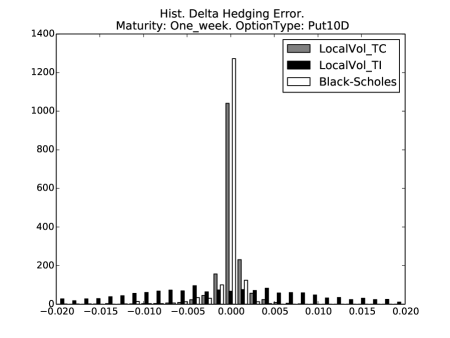
(a)

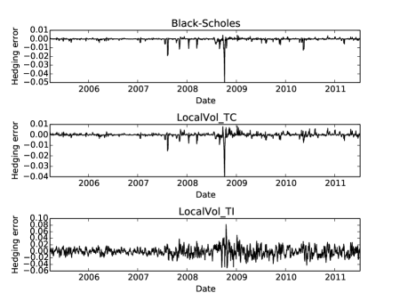
(b)

Figure 1: Delta hedging errors for (10$\Delta$Put) calls with one week maturity. LocalVol_TC and LocalVol_TI denote results from the theoretically correct and theoretically incorrect (sticky delta) local volatility models, respectively.

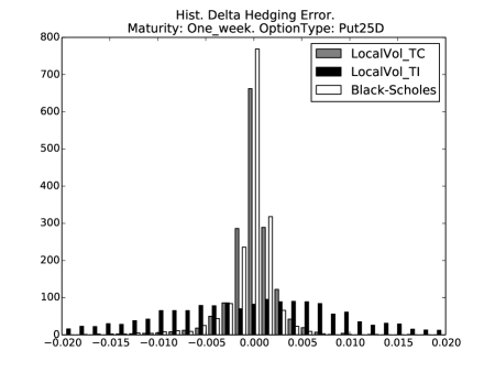
(a)

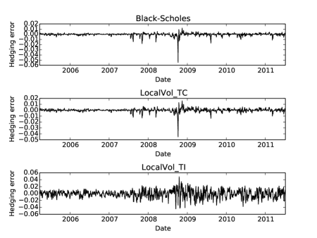
(b)

Figure 2: Delta hedging errors for (25$\Delta$Put) calls with one week maturity.

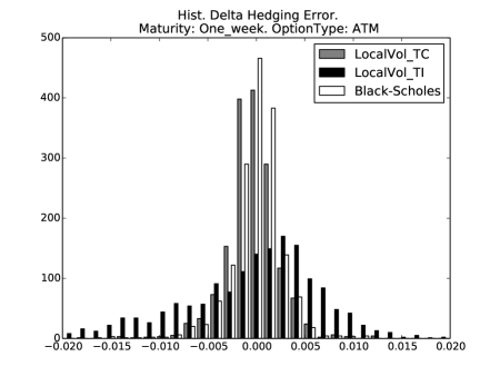
(a)

(b)

Figure 3: Delta hedging errors for ATM calls with one week maturity.

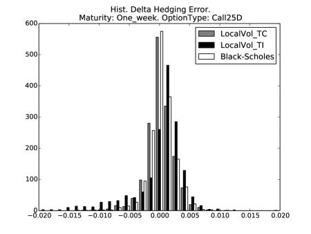
(a)

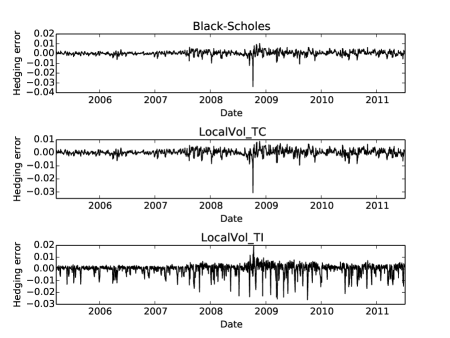
(b)

Figure 4: Delta hedging errors for (25$\Delta$Call) calls with one week maturity.

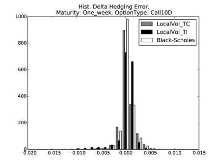
(a)

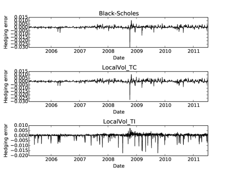
(b)

Figure 5: Delta hedging errors for (10$\Delta$Call) calls with one week maturity.

(a)

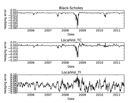
(b)

Figure 6: Delta hedging errors for (10$\Delta$Put) calls with one month maturity.

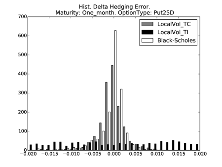
(a)

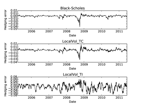
(b)

Figure 7: Delta hedging errors for (25$\Delta$Put) calls with one month maturity.

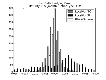
(a)

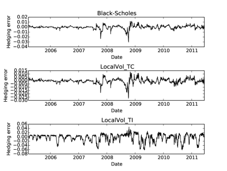
(b)

Figure 8: Delta hedging errors for ATM calls with one month maturity.

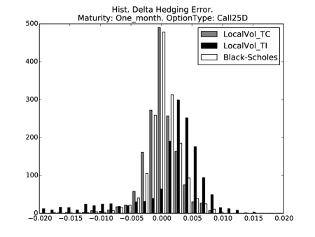
(a)

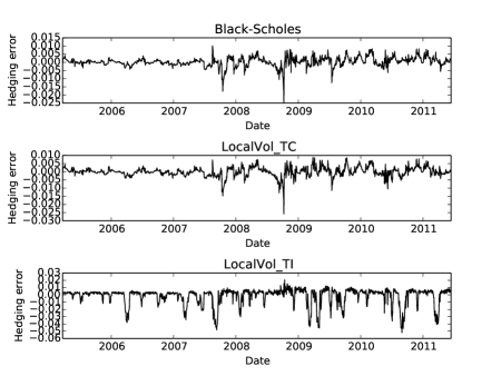
(b)

Figure 9: Delta hedging errors for (25$\Delta$Call) calls with one month maturity.

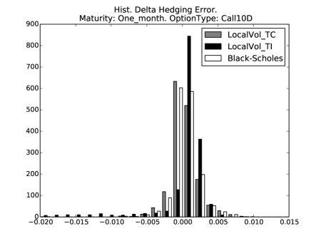
(a)

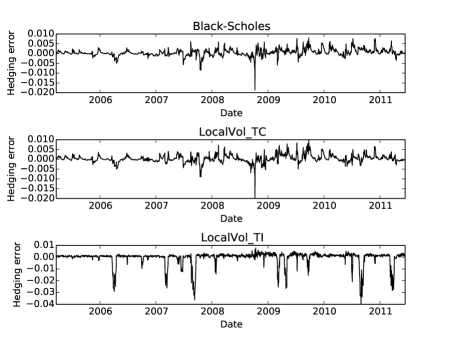
(b)

Figure 10: Delta hedging errors for (10$\Delta$Call) calls with one month maturity.

Delta	Model	Mean	Std. dev.
$10\Delta$Put	Black-Scholes	-0.0004	0.0024
$10\Delta$Put	LocalVol_TC	-0.0001	0.0023
$10\Delta$Put	LocalVol_TI	-0.001	0.0129
$25\Delta$Put	Black-Scholes	-0.0004	0.0029
$25\Delta$Put	LocalVol_TC	-0.0001	0.0028
$25\Delta$Put	LocalVol_TI	-0.0009	0.0108
ATM	Black-Scholes	-0.0	0.0028
ATM	LocalVol_TC	-0.0003	0.0028
ATM	LocalVol_TI	-0.0008	0.0078
$25\Delta$Call	Black-Scholes	0.0003	0.0023
$25\Delta$Call	LocalVol_TC	0.0002	0.0024
$25\Delta$Call	LocalVol_TI	-0.0	0.0046
$10\Delta$Call	Black-Scholes	0.0003	0.0016
$10\Delta$Call	LocalVol_TC	0.0003	0.0016
$10\Delta$Call	LocalVol_TI	0.0003	0.002

Table 3: Mean and standard deviation of hedging errors for each model under consideration for one week maturity.

Delta	Model	Mean	Std. dev.
$10\Delta$Put	Black-Scholes	-0.0012	0.005
$10\Delta$Put	LocalVol_TC	-0.0006	0.004
$10\Delta$Put	LocalVol_TI	-0.0063	0.0275
$25\Delta$Put	Black-Scholes	-0.0008	0.0041
$25\Delta$Put	LocalVol_TC	-0.0005	0.0039
$25\Delta$Put	LocalVol_TI	-0.0051	0.0236
ATM	Black-Scholes	-0.0002	0.0036
ATM	LocalVol_TC	-0.0006	0.0036
ATM	LocalVol_TI	-0.0035	0.0177
$25\Delta$Call	Black-Scholes	0.0003	0.0029
$25\Delta$Call	LocalVol_TC	-0.0001	0.0029
$25\Delta$Call	LocalVol_TI	-0.0016	0.0114
$10\Delta$Call	Black-Scholes	0.0005	0.0018
$10\Delta$Call	LocalVol_TC	0.0003	0.002
$10\Delta$Call	LocalVol_TI	-0.0005	0.0061

Table 4: Mean and standard deviation of hedging errors for each model under consideration for one month maturity.

10 Results

Figures 1 to 10 depict histograms of delta hedging errors computed from the historical data under the frameworks of Black-Scholes and local volatility. Within each histogram LocalVol_TC and LocalVol_TI denote the theoretically correct delta and sticky delta approaches, respectively. Sample means and standard deviations for these hedging errors are summarised in Tables 3 and 4.

We note that for in and at-the-money options (figures 1 to 3 for one week maturity and figures 6 to 8 for one month maturity), that the local volatility model with sticky delta performs significantly worse to the other two methods. It is only with deep in-the-money options (figure 5a) that sticky delta local volatility exhibits hedging errors better than Black-Scholes.

11 Conclusion

Using delta hedging as the criterion to measure the effectiveness of a market model, our results show that Black-Scholes is no worse than the local volatility model. In fact the Black-Scholes model performs significantly better than sticky delta local volatility, particularly for in and at-the-money options. The theoretically correct delta local volatility model gives hedging errors which are not too far from that of Black-Scholes and stick delta local volatility performs noticeably worse than the other models except for the case of deep out of the money options.

Further avenues of research include performing these empirical tests on other FX pairs and also incorporating other hedges such as vega. Also the framework can be used to validate/compare other models such as stochastic volatility, local stochastic volatility etc. It will also be of interest to determine hedging errors for exotic options such as barrier options.

References

- [1] F. Black and M. Scholes, “The pricing of options and corporate liabilities,” Journal of Political Economy, vol. 81, no. 3, pp. 637–654, 1973.
- [2] P. Wilmott, Paul Wilmott on Quantitative Finance. Wiley, 2007.
- [3] P. V. Shevchenko, “Advanced monte carlo methods for pricing european-style options,” CSIRO Mathematical and Information Sciences, CMIS Technical Report CMIS 2001/148, 2001.
- [4] W. H. Press, S. A. Teukolsky, W. T. Vetterling, and B. P. Flannery, Numerical recipes, 3rd ed. Cambridge: Cambridge University Press, 2007.
- [5] P. Glasserman, Monte Carlo methods in financial engineering. New York: Springer, 2003, vol. 53.
- [6] P. S. Hagan, D. Kumar, A. S. Lesniewski, and D. E. Woodward, “Managing smile risk,” Wilmott Magazine, pp. 84–108, 2002.
- [7] R. Rebonato, Volatility and correlation :the perfect hedger and the fox, 2nd ed. Wiley, 2005.
- [8] M. R. Fengler, Semiparametric modeling of implied volatility. Berlin: Springer-Verlag, 2005.