SU(2) Ginzburg-Landau theory for degenerate Fermi gases with synthetic non-Abelian gauge fields

Abstract

The non-Abelian gauge fields play a key role in achieving novel quantum phenomena in condensed-matter and high-energy physics. Recently, the synthetic non-Abelian gauge fields have been created in the neutral degenerate Fermi gases, and moreover, generate many exotic effects. All the previous predictions can be well understood by the microscopic Bardeen-Cooper-Schrieffer theory. In this work, we establish an SU(2) Ginzburg-Landau theory for degenerate Fermi gases with the synthetic non-Abelian gauge fields. We firstly address a fundamental problem how the non-Abelian gauge fields, imposing originally on the Fermi atoms, affect the pairing field with no extra electric charge by a local gauge-field theory, and then obtain the first and second SU(2) Ginzburg-Landau equations. Based on these obtained SU(2) Ginzburg-Landau equations, we find that the superfluid critical temperature of the intra- (inter-) band pairing increases (decreases) linearly, when increasing the strength of the synthetic non-Abelian gauge fields. More importantly, we predict a novel SU(2) non-Abelian Josephson effect, which can be used to design a new atomic superconducting quantum interference device.

The non-Abelian gauge fields, whose different components do not commute each other, are a central building block of the theory of fundamental interactions. Attributed to their high degrees of controllability, tunability, and versatility, ultracold quantum gases are a powerful platform to simulate the non-Abelian gauge fields. In general, the atomic quantum gases are charge neutral, and are thus not influenced by external gauge fields the way electrons are. Fortunately, by controlling different laser-atom interactions, the synthetic non-Abelian gauge fields can be created in these neutral quantum gases RJ95 ; JD11 ; NG14 . Moreover, the simplest non-Abelian gauge field, which is always called the one-dimensional (1D) equal-Rashba-Dresselhaus(ERD)-type spin-orbit coupling, has been realized experimentally YJL11 ; JYZ12 ; CQ13 ; JSC14 ; CH14 ; PW12 ; RAW13 ; ZF14 ; LWC12 , using a pair of Raman lasers. Recently, the similar but spatial-dependent gauge field has also been achieved in ultracold ⁸⁷Rb atom MCB13 . These important experiments pave a new way for exploring nontrivial quantum effects, induced by the synthetic non-Abelian gauge fields, in ultracold quantum gases. For instance, based on the microscopic Bardeen-Cooper-Schrieffer (BCS) theory, exotic superfluids RYW12 ; YZQ11 ; HH11 ; VJP11 ; HL12 ; WF13L ; WF13A ; YX14 ; MG11 ; MG12 ; KS12 ; HH13 ; CC13 ; CQU13 ; WZ13 ; XJL13 ; CCF14 ; HH14 , including the topological BCS MG11 ; MG12 ; KS12 ; HH13 ; CC13 and Fulde-Ferrell-Larkin-Ovchinnikov phases CQU13 ; WZ13 ; XJL13 ; CCF14 ; HH14 , have been predicted in degenerate Fermi gases.

In the conventional charge superconductors, the U(1) Ginzburg-Landau (GL) theory, in parallel with the microscopic BCS theory, is another famous theory to explore relevant physics MC73 . One of its most powerful features that it can be used to quantitatively describe the effects induced thermal fluctuations in the intermediate and strong coupling normal states, which are, however, missed in the BCS theory CAR93 . Moreover, some novel quantum phenomena, such as Josephson effect, flux flow, and the melting of the Abrikosov vortex lattice, etc. JFA04 , have also been revealed by this theory. However, the GL theory for degenerate Fermi gases with the synthetic non-Abelian gauge fields is still lacking. In this work, we establish an SU(2) GL theory for this system, based on the non-Abelian properties of the synthetic gauge fields.

Notice that in the conventional charge superconductors, the pairing has the electric charge $2e$, and is thus affected easily by the external gauge fields. However, the formed pairing in degenerate Fermi gases is charge neutral. It is natural to ask a fundamental and very important problem how the neutral pairing field interacts with the synthetic non-Abelian gauge fields, imposing originally on the Fermi atoms. We firstly address this key issue by a local gauge-field theory of the pairing field. Then, we obtain the first and second SU(2) GL equations by the variation of the total free energy with respect to the pairing field and the synthetic non-Abelian gauge fields. Based on these obtained SU(2) GL equations, we find that the superfluid critical temperature of the intra- (inter-) band pairing increases (decreases) linearly, when increasing the strength of the synthetic non-Abelian gauge fields. More importantly, we predict a novel SU(2) non-Abelian Josephson effect, which can be used to design a new atomic superconducting quantum interference device.

Results

Total free energy in space. In general, the pairing field, resulting from the two-component Fermi atom field $\phi(\mathbf{r})$ coupled with the synthetic SU(2) non-Abelian gauge fields, is expressed as $\psi(\mathbf{R})=\phi_{1}(\mathbf{r})\phi_{2}(\mathbf{r}^{\prime})$, where $\phi_{1}$ and $\phi_{2}$ are the fields for two different Fermi atoms, $\mathbf{r}$ is the 3D space-dependent coordinate of the Fermi atom, and $\mathbf{R}=(\mathbf{r}+\mathbf{r}^{\prime})/2$ is the coordinate of the pairing field AJL06 . Obviously, $\psi$ is a boson field. In terms of the local gauge-field theory of the pairing field (see Methods), we demonstrate strictly that this pairing field has an internal helical doublet and can interact with the same synthetic non-Abelian gauge fields, imposing originally on the Fermi atoms.

In addition, the total free energy is derived, in units of $\hbar=c=1$, by (see Methods)

$$F_{\text{s}}=\int d^{3}\mathbf{R(}f_{\text{n}}+U_{\text{eff}}+f_{\text{c}}+f_{\text{G}}).$$ (1)

In equation (1), $f_{\text{n}}$ is the energy density of the normal state. $U_{\text{eff}}=a\psi^{\ast}\psi+b(\psi^{\ast}\psi)^{2}/2$, with the coefficients $a$ and $b$, is the effective potential of the pairing field. The first and second terms of $U_{\text{eff}}$ are the free and self-interacting energy densities of the pairing field, respectively. The explicit expressions of the coefficients $a$ and $b$ can, in principle, be determined from the microscopic BCS theory AJL06 . In general, the coefficient $a$ is dependent of temperature. When the temperature is lower than the superfluid critical temperature, $a>0$, while $a<0$ vice versa. On contrary, the coefficient $b$ is positive for any temperature. $f_{\text{c}}=\left|\Pi_{i}\psi\right|^{2}/4m$ is the kinetic energy, where $\Pi_{i}=-i\partial_{i}-\alpha A_{i}$ and $m$ is the mass of the Fermi atom. $f_{\text{G}}=\varrho L_{ij}L_{ij}$ is the energy density functional of the synthetic non-Abelian gauge fields $A_{i}$, where $L_{ij}=\Pi_{i}A_{j}-\Pi_{j}A_{i}$ is the tensor of the synthetic non-Abelian gauge fields $A_{i}$, and satisfies the anti-symmetry property $L_{ij}=-L_{ji}$, and $\varrho$ is a coefficient determined by the synthetic non-Abelian gauge fields $A_{i}$. In the previous discussions, the synthetic non-Abelian gauge fields are usually chosen, in the spin-basis representation, as

$$\mathbf{A}=[l\sigma_{x},\chi l\sigma_{y},0,f(l)\text{\^{I}}_{2}\mathbf{]},$$ (2)

where $l$ and $f(l)$ are the introduced functions of space-time, the dimensionless constant $\chi$ determines the type of the synthetic non-Abelian gauge fields, and Î₂ is a $2\times 2$ unit matrix. For $\chi=1$, the 2D RD-type non-Abelian gauge field emerges, and becomes the 1D ERD-type non-Abelian gauge field in the case of $\chi=0$ YJL11 ; JYZ12 ; CQ13 ; JSC14 ; CH14 ; PW12 ; RAW13 ; ZF14 ; LWC12 . Recent experiment shows that the functions $l$ and $f(l)$ can be determined by the Rabi frequencies of laser fields MCB13 , thus both space- and time- dependent functions $l$ and $f(l)$ can be accessible.

The first SU(2) GL equation. To describe the stable superfluid, we need study the variations of the total free energy, $\delta F_{\text{s}}(\psi)$, $\delta F_{\text{s}}(\psi^{\ast})$, and $\delta F_{\text{s}}(A_{i})$. In the case of the three-component non-Abelian gauge fields $A_{i}$, the results are very complicate. For simplicity, here we only deal with the in-plane non-Abelian gauge fields, i.e., $A_{z}=0$. In such a case, we obtain the first SU(2) GL equation (see Methods)

$$\frac{1}{4m}\left[(-i\partial_{\zeta}-\alpha A_{\zeta})^{2}-\partial_{z}^{2}\right]\psi+a\psi+b\psi^{2}\psi=0$$ (3)

with $\zeta=x,y$.

The gauge-invariant field equation (3) fully describes the interplay between neutral superfluids and the synthetic non-Abelian gauge fields, when the temperature is lower than the superfluid critical temperature. It seems that this equation is similar to that of the U(1) case. In fact, the physics is quite different. Attributed to the SU(2) properties of the synthetic gauge fields, there are two kinds of superfluid states, including the positive and negative helical states. Moreover, they couple with each other and both of them are vectors in 2D Hilbert space of the helical basis. It means that equation (3) is a two-component coupled equation in 2D Hilbert space. In addition, in the U(1) case, the pairing is formed by two spin states. However, in the presence of the synthetic non-Abelian gauge fields, the pairing emerges in two helical states. These different spin and helical states lead to different dispersion relations, and thus different microscopic quantum statistics of the interacting many-body systems. It implies that the coefficients $a$ and $b$ are also different.

Due to existence of the term $b\psi^{2}\psi$, the two-component nonlinear equation (3) is hard to be solved exactly. Here we use an approximate linearization method (i.e., assuming $b\psi^{2}\psi\simeq 0$) to deal with this equation AAA57 ; BR10 . As an example, we consider a static RD-type non-Abelian gauge field, i.e., $l=1$ and $\chi=1$ in equation (2). In such case, we rewrite the spatial part of this non-Abelian gauge field as $[\sigma_{x}k_{\text{F}}(\xi_{0}+\varkappa y),\sigma_{z}k_{\text{F}}(\xi_{0}+\varkappa x),0\mathbf{]}$, with the dimensionless infinitesimal $\varkappa$ and the Fermi vector $k_{\text{F}}$ of the non-interacting Fermi gases, and then assume the corresponding solution as $\psi=\exp(ik_{z}z)h(x,y)$. The introduced dimensionless infinitesimal $\varkappa$ doesn’t change the static property of the RD-type non-Abelian gauge field since $\varkappa y\longrightarrow 0$ and $\varkappa x\rightarrow 0$, but is an auxiliary quality, which only help us to approximately solve equation (3). Substituting the assumed solution $\psi$ into equation (3) and using the approximate linearization method AAA57 ; BR10 , we obtain the following 2D oscillator-type equation: $-(\partial_{x}^{2}+\partial_{y}^{2})h(x,y)/4m+m\varkappa^{2}[\omega_{cy}^{2}(y-C_{0})^{2}+\omega_{cx}^{2}(x-C_{0})^{2}]h(x,y)=(\left|a\right|-k_{z}^{2}/4m)h(x,y)$, where $\omega_{cx}=\alpha\sigma_{z}k_{\text{F}}/2m$ and $\omega_{cy}=\alpha\sigma_{x}k_{\text{F}}/2m$ are the circular frequencies in the $x$ and $y$ directions, respectively, and $C_{0}=-\xi_{0}/\varkappa$. By further solving the above oscillator-type equation, we obtain $\left|a\right|-k_{z}^{2}/4m$ $=(n_{x}^{\prime}+1/2)\omega_{cx}+(n_{y}^{\prime}+1/2)\omega_{cy}$, where $n_{x}^{\prime}$ and $n_{y}^{\prime}$ are the positive integers. When the condensate occurs, only the ground state ($n_{x}^{\prime}=n_{y}^{\prime}=0$, $k_{z}=0$) becomes significant AAA57 ; BR10 . As a consequence, the critical temperature is obtained, in the spin-basis representation, by $T_{c}^{\text{s}}\simeq T_{c}(0)-\alpha k_{\text{F}}(\sigma_{x}+\sigma_{z})/4a_{T}m$, where $T_{c}(0)$ is the critical temperature without the synthetic non-Abelian gauge fields, and $a_{T}(>0)$ is the leading-order expansion coefficient of $a$ at $T_{c}(0)$.

Since in this work we investigate the physics of superfluid with the helical doublet, the critical temperature is obtained, from a transformation of SU(2) group representation to the helical basis of pairing doublet, by

$$T_{c}\simeq T_{c}(0)-\frac{\sqrt{2}\alpha k_{\text{F}}\sigma_{z}}{4a_{T}m}.$$ (4)

When $\alpha=0$, $T_{c}=T_{c}(0)$, as expected. Equation (4) shows that the superfluid critical temperature is a $2\times 2$ matrix, because equation (3) is a two-component coupled equation. The diagonal elements reflect the critical temperature for the different superfluid states (the positive and negative helical states). Using the similar consideration of the electric charge matrix of the left-handed doublet of lepton SW67 , we find that, when increasing the coupling strength $\alpha$, the critical temperature of the pairing field in the negative helical state increases linearly from a non-zero value, which is consistent with the result derived from the microscopic BCS theory with the Nozieŕes–Schmitt-Rind correction RYW12 . Moreover, we can confirm that the pairing fields in the positive and negative helical states govern the superfluid physics of the inter- and intra- band pairings, respectively. For the superfluid critical temperature of the inter-band pairing, it decreases linearly when increasing the coupling strength $\alpha$. This behavior can also be easily understood since the inter-band pairing is gradually suppressed, attributed to the blocking effect in Fermi surface.

The second SU(2) GL equation. The second SU(2) GL equation is obtained by (see Methods)

$$\frac{i\alpha}{4m}(\psi^{\ast}\partial_{\zeta}\psi-\psi\partial_{\zeta}\psi^{\ast})+\frac{\alpha^{2}}{2m}\psi^{\ast}\psi A_{\zeta}=2\varrho(\Lambda_{\zeta}-i2\alpha\Theta_{\zeta}),$$ (5)

where

$$\Lambda_{\zeta}=\partial_{\eta}\partial_{\zeta}A_{\eta}-\partial_{\eta}^{2}A_{\zeta}-\partial_{z}^{2}A_{\zeta},$$ (6)

$$\Theta_{\zeta}=-(\partial_{\zeta}A_{\eta})A_{\eta}+(\partial_{\eta}A_{\zeta})A_{\eta}$$ (7)

with $\eta=x,y$. Equation (5) is also a two-component field equation. The left term of this equation reflects the in-plane supercurrents AJL06 , i.e,

$$j_{\zeta}=\frac{i\alpha}{4m}(\psi^{\ast}\partial_{\zeta}\psi-\psi\partial_{\zeta}\psi^{\ast})+\frac{\alpha^{2}}{2m}\psi^{\ast}\psi A_{\zeta},$$ (8)

This means that equation (5) governs the interplay between the in-plane supercurrents $j_{\zeta}$ and the synthetic non-Abelian gauge fields $A_{\zeta}$. In addition, the term $\Theta_{\zeta}$ in equation (7) is a new term, originating from the non-Abelian properties of the synthetic gauge fields $A_{\zeta}$. The supercurrent in the $z$ direction is given by (see Methods)

$$j_{z}=\frac{i\alpha}{4m}(\psi^{\ast}\partial_{z}\psi-\psi\partial_{z}\psi^{\ast}).$$ (9)

In terms of Noether’s theorem LR96 , the neutral supercurrents in equations (8) and (9) are the SU(2) charge currents, rather than the conventional probability currents ($j_{i}=n_{0}\partial_{i}\theta/2m$) of superfluid order parameter $\psi_{0}=\sqrt{n_{0}}e^{i\theta}$ without any gauge field, where $n_{0}$ is the density of pairing. However, the supercurrent in the $z$ direction is trivial, since it doesn’t interact with the synthetic non-Abelian gauge fields $A_{\zeta}$. When the synthetic gauge fields are the U(1) cases, the term $\Theta_{\zeta}=0$, and equations (3) and (5) reduce respectively to $\left[(-i\partial_{\zeta}-e^{\prime}A_{\zeta})^{2}-\partial_{z}^{2}\right]\psi/4m+a\psi+b\psi^{2}\psi=0$ and $ie^{\prime}(\psi^{\ast}\partial_{\zeta}\psi-\psi\partial_{\zeta}\psi^{\ast})/4m+e^{\prime 2}\psi^{\ast}\psi A_{\zeta}/2m=2\varrho\Lambda_{\zeta}$, where $e^{\prime}$ is the effective electric charge AJL06 . Moreover, the pairing field $\psi$ is a single-component scalar field.

We emphasize that the nonlinear SU(2) GL equation (5) is gauge invariant, even if the terms $\Lambda_{\zeta}\$and $\Theta_{\zeta}$ are dependent of the synthetic non-Abelian gauge fields. Notice that for the static synthetic non-Abelian gauge fields, $\Lambda_{\zeta}=0$ and $\Theta_{\zeta}=0$, derived from equations (6)-(7). It seems that the in-plane supercurrents vanish. In fact, in terms of SU(2) symmetry, we make a local gauge transformation $\psi^{\prime}=U_{L}\psi$ and $A_{i}^{\prime}=-i(\partial_{i}U_{L})U_{L}^{{\dagger}}/\alpha+U_{L}A_{i}U_{L}^{{\dagger}}$, and then obtain $\Lambda_{\zeta}^{\prime}\neq 0$ and $\Theta_{\zeta}^{\prime}\neq 0$, i.e., equation (5) as well as the in-plane supercurrents still exist.

If the synthetic non-Abelian gauge fields are dependent of space-time, they can not be transformed to the static cases by a local gauge transformation. In this case, the superfluid physics becomes very rich, and however, is difficult to be discussed by the microscopic BCS theory. On contrary, our established GL theory is a powerful tool in this respect. In the Table I, we give the explicit expressions of $\Lambda_{\zeta}$, $\Theta_{\zeta}$, and especially, the supercurrents for the 2D RD- and 1D ERD- type non-Abelian gauge fields with $l=\Sigma t+\varepsilon\sin(\omega_{0}t)/\omega_{0}$, where the physical meanings of parameters $\Sigma$, $\varepsilon$, and $\omega_{0}$ will be interpreted in the following discussions. For the 1D ERD-type non-Abelian gauge field, the new term $\Theta_{\zeta}$ disappears. In addition, we will show in the next section that the space-time-dependent non-Abelian gauge fields generate a novel SU(2) non-Abelian Josephson effect, which is a tunneling phenomenon in a weakly-linked superfluid system BD65 .

SU(2) non-Abelian Josephson effect. To predict the SU(2) non-Abelian Josephson effect, we consider two identical degenerate Fermi gases without initial population imbalance, respectively distributed in two sides of double-well potential through a weakly-linked barrier LS07 ; AM05 ; SA07 ; HH111 , and denote these two regions as I and II (see Fig.1). The space-time-dependent non-Abelian gauge fields are chosen as the terms in equation (2). In this neutral Fermi atom system, we can investigate a gauge-invariant mass current $j_{\zeta}^{m}=2mj_{\zeta}$, where the factor $2$ originates that the formed pairing consists of two atoms BPA98 ; FSC01 .

[t] The explicit expressions of $\Lambda_{\zeta}$, $\Theta_{\zeta}$, and especially, the supercurrents for the 2D RD- and 1D ERD- type non-Abelian gauge fields. The supercurrent 1 can be influenced by the synthetic non-Abelian gauge fields, while the supercurrent 2 is only a trivial SU(2) charge current, like Eq. (9). In the case of the 1D ERD-type non-Abelian gauge field, the new term $\Theta_{\zeta}$ disappears, and the supercurrent 1 emerges only in the $x$ direction. Here, the functions are defined as $y_{1}=\Sigma t^{2}\partial_{\eta}\Sigma+t\partial_{\eta}(\Sigma\varepsilon)\sin(\omega_{0}t)/\omega_{0}$ and $y_{2}=\varepsilon\partial_{\eta}\varepsilon\sin^{2}(\omega_{0}t)/\omega_{0}^{2}$, respectively. The indices $\zeta$ and $\eta$ satisfy the Einstein rule, in which $\zeta$ and $\eta$ only take different coordinates of $x$ and $y$ at the same time, i.e., if $\zeta=x$, then $\eta=y$. ERD RD SU(2) gauge fields $(l\sigma_{x},0,0)$ $(l\sigma_{x},l\sigma_{y},0)$ ${\Lambda}_{\zeta}$ $-(\partial_{y}^{2}+\partial_{z}^{2})l\sigma_{x}$ $-(\partial_{\eta}^{2}+\partial_{z}^{2})l\sigma_{\zeta}$ $\Theta_{\zeta}$ $0$ $(y_{1}+y_{2})(\sigma_{\zeta}\sigma_{\eta}-\hat{I})$ Supercurrent 1 $j_{x}^{\text{ERD}}$ $j_{x}^{\text{RD}}$, $j_{y}^{\text{RD}}$ Supercurrent 2 $j_{y}^{\text{ERD}}$, $j_{z}^{\text{ERD}}$ $j_{z}^{\text{RD}}$

When the vacuum condensate occurs, we have two conditions, $\partial U_{\text{eff}}/\partial\psi=0$ and $\partial U_{\text{eff}}/\partial\psi^{\ast}=0$ LR96 , and thus $\psi^{\ast}\psi=-a/b$. So the pairing field is written as $\psi=(\sqrt{a/4b},\sqrt{a/4b})^{T}e^{i(\frac{\pi}{2}+\varphi)}$, where $\varphi$ is the phase. In addition, in this weakly-linked system, we also have two phenomenal boundary conditions, $\partial\psi_{\text{I}}/\partial\zeta=\psi_{\text{II}}/d^{\prime}$ and its complex conjugate, at the barrier MC73 , where the parameter $d^{\prime}$ is the width of barrier. Without the synthetic non-Abelian gauge fields $A_{\zeta}$, the direct-current Josephson mass current density in the $\zeta$ direction is found as $j_{\zeta}^{m}=-(a\alpha/2bd^{\prime})\hat{\Xi}\sin(\Delta\varphi)$, where the phase difference is defined as $\Delta\varphi\mathbf{=}\varphi_{\text{II}}-\varphi_{\text{I}}$ and $\hat{\Xi}$ is a $2\times 2$ matrix with $\hat{\Xi}_{11}=\hat{\Xi}_{12}=\hat{\Xi}_{21}=\hat{\Xi}_{22}=1$. In the presence of the synthetic non-Abelian gauge fields $A_{\zeta}$, the phase difference must be modified, in order to obtain the gauge-invariant mass current. By considering the dimensional property, we write a gauge-invariant phase difference as $\Delta\varphi=\varphi_{\text{II}0}-\varphi_{\text{I}0}-\alpha\int\nolimits_{\text{I}}^{\text{II}}A_{\zeta}d\zeta$, where $\Delta\Phi_{0}=\varphi_{\text{II}0}-\varphi_{\text{I}0}$ is the initial phase difference between the regions I and II. Since the synthetic non-Abelian gauge fields $A_{\zeta}$ are dependent of space-time, we further rewrite the total phase difference as $\Delta\mathbf{\varphi=}-\alpha\int_{t_{0}}^{t}dt\int\nolimits_{\text{I}}^{\text{II}}\frac{dA_{\zeta}}{dt}d\zeta$ , and the mass current is thus given by

$$j_{\zeta}^{m}=-\frac{a\alpha}{2bd^{\prime}}\left[\begin{array}[]{cc}1&1\\ 1&1\end{array}\right]\sin\mathbf{(-}\alpha\mathbf{\left[\begin{array}[]{cc}0&\kappa_{1}\\ \kappa_{2}&0\end{array}\right]),}$$ (10)

where $\kappa_{1}=\int_{t_{0}}^{t}dt\int\nolimits_{\text{I}}^{\text{II}}\lambda_{1}\frac{dl}{dt}d\zeta$, $\kappa_{2}=\int_{t_{0}}^{t}dt\int\nolimits_{\text{I}}^{\text{II}}\lambda_{2}\frac{dl}{dt}d\zeta$, and $\lambda_{1}$ and $\lambda_{2}$ are the dimensionless constants, determined by the type of the synthetic non-Abelian gauge fields. For the ERD-type ($\chi=0$) or the $x$ component of the RD-type ($\chi=1$) non-Abelian gauge fields, $\lambda_{1}=\lambda_{2}=1$, which become $\lambda_{1}=-i$ and $\lambda_{2}=i$ in the case of the $y$ component of the RD-type non-Abelian gauge field.

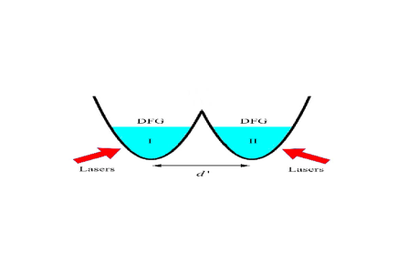
Figure 1: A possible scheme to achieve the SU(2) non-Abelian Josephson effect and the Shapiro step. Two identical degenerate Fermi gases (DFGs) without initial population imbalance are respectively distributed in two sides of the double-well potential. The lasers are used to create the non-Abelian gauge fields.

By controlling different laser-atom interactions (for example, adding a sinusoidal perturbation on Rabi frequencies, etc.) RJ95 ; JD11 ; NG14 , we can choose $dl/dt=\Sigma+\varepsilon\cos(\omega_{0}t)$ with $\Sigma=dG/d\zeta$ and $\varepsilon=dg/d\zeta$, where $G$ and $g$ reflect the chemical potential difference between the two wells of the unit SU(2) charge in the synthetic non-Abelian gauge fields and its amplitude of oscillating potential perturbation, respectively. In this case, the coefficient $\varrho=\omega_{0}d^{\prime 4}/4$. When $\{G,g\}\ll E_{\text{F}}$ ($E_{\text{F}}=k_{\text{F}}^{2}/2m$ is the Fermi energy of the non-interacting gases), equation (10) is simplified as (see Methods)

$$j_{\zeta}^{m}=-\frac{a\alpha}{2bd^{\prime}}\hat{\Xi}\sum\limits_{k=-\infty}^{\infty}\hat{\Omega}_{k}$$ (11)

with $\hat{\Omega}_{k}=$diag$(\kappa_{3},\kappa_{4})$, where $\kappa_{3}=\lambda_{1}\lambda_{2}(-1)^{k}J_{k}(\alpha g/\omega_{0})\sin[(\alpha G-k\omega_{0})t+\alpha\Delta\varphi_{01})]$, $\kappa_{4}=\lambda_{1}\lambda_{2}(-1)^{k}J_{k}(\alpha g/\omega_{0})\sin[(\alpha G-k\omega_{0})t+\alpha\Delta\varphi_{02})]$, $J_{k}(\alpha g/\omega_{0})$ is the $k$-th Bessel function with respect to $\alpha g/\omega_{0}$, and $\Delta\varphi_{01}$ and $\Delta\varphi_{02}$ are the matrix elements of the initial phase difference. Equation (11) shows that the space-time-dependent synthetic non-Abelian gauge fields can induce an alternating-current SU(2) Josephson mass current, which has never been predicted from the microscopic BCS theory YZQ11 ; HH11 ; VJP11 ; HL12 ; RYW12 ; WF13L ; WF13A ; YX14 ; MG11 ; MG12 ; KS12 ; HH13 ; CC13 ; CQU13 ; WZ13 ; XJL13 ; CCF14 ; HH14 .

In equation (11), if $\alpha G-k\omega_{0}=0$, the $k$-th current, with the magnitude $I_{k}=\left|a\alpha J_{k}(\alpha g/\omega_{0})/2bd^{\prime}\right|$, converts to a direct current. This means that the Shapiro step, with the same magnitude $I_{k}$, emerges in our predicted mass-current Josephson effect. We define a $k$-th gap $\Delta_{k}=\alpha G_{0}-k\omega_{0}=N\omega_{0}$, where $N\in\mathbb{Z}$ is a topological invariant of the fundamental group $\pi_{1}(S^{1})$ with $S^{1}=\mathbf{\mathbb{\mathbb{R}}}^{1}\cup\{\infty\}$. We find that the direct-current component is topologically trivial ($N=0$) and the alternating-current component is topologically nontrivial ($N\neq 0$). When increasing $G$, we need consider a generalized gap $\Delta_{k}=(N+\sigma)\omega_{0}$, where $\sigma\in[0,1]$. When $\sigma=1$, the $k$-th component becomes topologically nontrivial ($N=1$), while the $(k+1)$-th component becomes topologically trivial ($N=0$), where a new Shapiro step, with the magnitude $I_{k+1}$, appears. This process is depicted in Fig. 2. We emphasize that our predictions arises from the space-time-dependent non-Abelian gauge fields. If the gauge field is chosen as the static Rashba-type gauge fields, $\Delta\zeta_{\text{II{,}I}}\simeq d^{\prime}$, and only a constant Josephson mass current emerges. This Josephson mass current is topologically trivial, as shown in the black solid line in Fig. 2.

Finally, we briefly illustrate the possible experimental observation of the predicted SU(2) non-Abelian Josephson effect and the corresponding Shapiro steps. In experiments, the double-well potential can be constructed effectively by the superposition of a 1D periodic optical lattice with a 3D magnetic harmonic trap. The frequencies in the radial and normal directions of the 3D magnetic trap are of $10^{3}$Hz and $10^{2}$Hz, respectively LLAS04 . The width and height of barrier are about $2\sim 4\mu m$ and of $10^{3}$Hz, respectively. When the pairing field condenses in the double-well potential with particle density $n=3\times 10^{13}cm^{-3}$, $G\sim 0.1E_{\text{F}}$ and $g\sim 0.05E_{\text{F}}$ MCC04 . This means the the condition $\{G,g\}\ll E_{\text{F}}$ is valid. Thus, the predicted SU(2) non-Abelian Josephson effect as well as the Shapiro steps can be detected experimentally by the way of non-destructive phase contrast image LS07 .

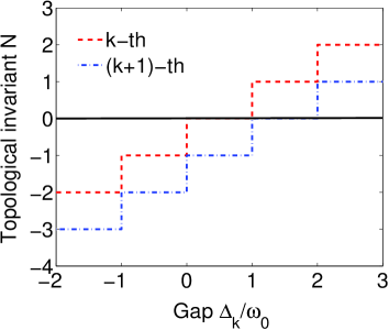
Figure 2: The evolution of the topological invariant of the current component in equation (11). The black line represents the topologically-trivial mass current in the presence of a static Rashba-type non-Abelian gauge field.

Discussion

In summary, we have demonstrated strictly that the neutral pairing of degenerate Fermi gases interacts with the same synthetic non-Abelian gauge fields, imposing originally on the Fermi atoms. Moreover, we have obtained the first and second SU(2) GL equations, which allow us to predict new quantum effects, such as an SU(2) non-Abelian Josephson effect and the corresponding Shapiro steps for the space-time-dependent non-Abelian gauge fields. These results give new applications of the synthetic non-Abelian gauge fields. For example, we can design a novel atomic direct-current superconducting quantum interference device RCB13 , based on the predicted SU(2) non-Abelian Josephson effect.

Methods

The local gauge theory of the pairing field. In order to apply the local gauge theory, we in this subsection consider the 4D space-time-dependent coordinate, i.e., $x_{\mu}=(t,\mathbf{r})$. We begin to study a two-component Fermi atom field $\phi(x_{\mu})$ coupled with the synthetic non-Abelian gauge field. When the massive Fermi atom field interacts with the synthetic non-Abelian gauge fields, its behavior is identical to a Dirac field with the same local gauge symmetry. In this Dirac-like atom field, each component reflects a spinor, corresponding to an internal helical state. The corresponding speace-time action is written as LR96

$$S=\int d^{4}x_{\mu}[\bar{\phi}i\gamma^{\mu}(\partial_{\mu}+i\alpha A_{\mu})\phi-m\bar{\phi}\phi-\frac{1}{4}F_{\mu\nu}F^{\mu\nu}].$$ (12)

In equation (12), $\gamma^{\mu}$ ($\mu=0,1,2,3$) are the Dirac gamma matrices, satisfying the Clifford algebra $\gamma^{\mu}\gamma^{\nu}+\gamma^{\nu}\gamma^{\mu}=\delta_{\mu\nu}$Î, where $\delta_{\mu\nu}$ and Î are the Kronecker notation and $4\times 4$ unit matrix, respectively. $\partial_{\mu}+i\alpha A_{\mu}$ are the covariant derivatives of the Fermi atom field $\phi$, where $A_{\mu}(x_{\mu})$ are the synthetic non-Abelian gauge fields with $[A_{\mu},A_{\nu}]\neq 0$, and $\alpha$ is a constant that governs the coupling between the Fermi atom field $\phi$ and the non-Abelian gauge fields $A_{\mu}$. $F_{\mu\nu}=\partial_{\mu}A_{\nu}-\partial_{\nu}A_{\mu}+i\alpha[A_{\mu},A_{\nu}]$ is the tensor of our considered non-Abelian gauge fields. The space-time action in equation (12) is invariant via a local gauge transformation $\phi^{\prime}=U_{L}\phi$, with $U_{L}(x_{\mu})=\exp[-i\Lambda^{\epsilon}(x_{\mu})\tau_{\epsilon}]$, where $\tau_{\epsilon}$ ($\epsilon=1,2,3$) are the generators of the SU(2) Lie group, and $\Lambda^{\epsilon}(x_{\mu})$ are the phase factors of space-time.

For the pairing field, we firstly investigate the global gauge symmetry, and then generalize it to the local case. When we introduce a global SU(2) operator $U_{G}=\exp(-i\Lambda_{G}^{a}\tau_{a})$, where $\Lambda_{G}^{a}$ is independent of space-time, to make a gauge transformation $\phi_{1}\rightarrow U_{G}\phi_{1}$ or $\phi_{2}\rightarrow U_{G}\phi_{2}$, the pairing field becomes $\psi\rightarrow U_{G}\phi_{1}\phi_{2}$, which means that $\psi^{\prime}=U_{G}\psi$. According to the principle of gauge-field theory, we should obtain a Lagrangian invariant $\mathcal{L}=T-V$, under the above global gauge transformation of the pairing field $\psi$. Using the relation $-i\partial_{\mu}\psi^{\prime}=-i\partial_{\mu}U_{G}\psi=-iU_{G}\partial_{\mu}\psi$ and its complex conjugate, we find directly that the kinetic energy $T=$ $(i\partial^{\mu}\psi^{\ast})(-i\partial_{\mu}\psi)$ is invariant. For the scalar pairing field $\psi$ that can condense in a non-zero vacuum state, the effective potential $V$ must have a stable and non-zero minimum point (vacuum). If expanding the effective potential $V$ with respect to $\psi^{\ast}\psi$ around the critical temperature $T_{c}$ (up to second order), we obtain $V\simeq-a\psi^{\ast}\psi-b(\psi^{\ast}\psi)^{2}/2$. Thus, the global gauge-invariant action for the pairing field $\psi$ is given by $S_{G}^{\psi}=\int d^{4}X_{\mu}[(i\partial^{\mu}\psi^{\ast})(-i\partial_{\mu}\psi)+U_{\text{eff}}]$, where $U_{\text{eff}}=-V$ is an effective potential LR96 .

To discuss the local gauge symmetry of the pairing field $\psi$, we replace $U_{G}$ by $U_{L}$ to make a similar gauge transformation. However, in such case, $-i\partial_{\mu}\psi^{\prime}\neq-iU_{L}\partial_{\mu}\psi$. As a result, we introduce new covariant derivatives of the paring field $\psi$, $D_{\mu}=-i\partial_{\mu}-\beta B_{\mu}$, to realize $(D_{\mu}\psi)^{\prime}=U_{L}(D_{\mu}\psi)$ LR96 , which gives rise to three following equations:

$$-i\partial_{\mu}(U_{L}\psi)-\beta B_{\mu}^{\prime}U_{L}\psi=-iU_{L}\partial_{\mu}\psi-\beta U_{L}B_{\mu}\psi,\text{c.c.},$$ (13)

and

$$B_{\mu}^{\prime}=-\frac{i}{\beta}(\partial_{\mu}U_{L})U_{L}^{{\dagger}}+U_{L}B_{\mu}U_{L}^{{\dagger}},$$ (14)

where c.c. is the complex conjugate. With the help of equation (14) and the covariant derivatives $D_{\mu}$, we confirm that $(D^{\mu}\psi^{\ast})(D_{\mu}\psi)$ are invariant under the local gauge transformation $U_{L}$, and so is the effective potential $U_{\text{eff}}$. As a consequence, we obtain the space-time action for the pairing field $\psi$ in the local gauge symmetry,

$$S_{L}^{\psi}=\int d^{4}X_{\mu}[(D^{\mu}\psi^{\ast})(D_{\mu}\psi)+U_{\text{eff}}+\mathcal{L}_{V}],$$ (15)

where $B_{\mu}$ are called the SU(2) Yang-Mills gauge fields, $\beta$ is a constant reflecting the coupling between the pairing field $\psi$ and the Yang-Mills gauge fields $B_{\mu}$, $\mathcal{L}_{V}=-V_{\mu\nu}V^{\mu\nu}/4$, with $V_{\mu\nu}=$ $D_{\mu}B_{\nu}-D_{\nu}B_{\mu}$, is the energy density invariant of the Yang-Mills gauge fields $B_{\mu}$.

Due to the identical gauge properties of the pairing field $\psi$ and the Fermi atom field $\phi$, the Yang-Mills gauge fields $B_{\mu}$ must have the same terms as the synthetic non-Abelian gauge fields $A_{\mu}$. Moreover, they have an identical conserved quality called the SU(2) charge, according to Noether’s theorem LR96 . This means that $\alpha=\beta$. The above two results lead to a significant conclusion that the pairing field $\psi$ can also couple identically with the non-Abelian gauge fields $A_{\mu}$, imposing originally on the Fermi atoms, and have a similar internal helical doublet, like the Fermi atoms. In addition, we obtain equation (1) in the text, by extracting the spatial part of the space-time action in equation (15).

The derivation of the first and second SU(2) GL equations. The variation of the total free energy functional can be written formally as

$$\delta F_{\text{s}}=\int d^{3}\mathbf{R(}\delta f_{\text{n}}+\delta U_{\text{eff}}+\delta f_{\text{c}}+\delta f_{\text{G}}).$$ (16)

When condensate of the pairing field $\psi$ occurs, $\delta f_{\text{n}}\equiv 0$. Since the effective potential density does not depend on the synthetic non-Abelian gauge fields, we have

$$\delta U_{\text{eff}}=\delta U_{\text{eff}}(\psi)+\delta U_{\text{eff}}(\psi^{\ast}).$$ (17)

If further neglecting the higher-order terms with respect to $\delta\psi$ and $\delta\psi^{\ast}$, we derive $\delta U_{\text{eff}}(\psi)=a\delta\psi\psi^{\ast}+b\delta\psi\psi^{\ast}\psi\psi$ and $\delta U_{\text{eff}}(\psi^{\ast})=a\psi\delta\psi^{\ast}+b\delta\psi^{\ast}\psi^{\ast}\psi^{\ast}\psi$.

For the coupled term between the pairing field $\psi$ and the synthetic non-Abelian gauge fields $A_{i}$, we have

$$\delta f_{\text{c}}=\delta f_{\text{c}}(\psi)+\delta f_{\text{c}}(\psi^{\ast})+\delta f_{\text{c}}(A_{i})\text{,}$$ (18)

where $i$ and $j$ run over $x$, $y$, and $z$, because the pairing has a 3D momentum. After a careful calculation, we have $\delta f_{\text{c}}(\psi)=\left[(\partial_{i}^{\ast}\psi^{\ast}+i\alpha A_{i}\psi^{\ast})\delta\psi-(\partial_{i}^{\ast}+i\alpha A_{i})^{2}\psi^{\ast}\delta\psi\right]/4m$ and $\delta f_{\text{c}}(\psi^{\ast})=\left[(\partial_{i}\psi-i\alpha A_{i}\psi)\delta\psi^{\ast}-(\partial_{i}-i\alpha A_{i})^{2}\psi\delta\psi^{\ast}\right]/4m$. On the other hand, when neglecting the higher-order terms with respect to $\delta A_{i}$, we obtain $\delta f_{\text{c}}(A_{i})\simeq\alpha^{2}\psi^{\ast}\psi\delta A_{i}A_{i}/2m+i\alpha(\psi^{\ast}\partial_{i}\psi\delta A_{i}-\psi\partial_{i}\psi^{\ast}\delta A_{i})/4m$.

Finally, we consider the variation of the energy functional density of the synthetic non-Abelian gauge fields $A_{i}$,

$$\delta f_{\text{G}}=\varrho\left[L_{ij}(\mathbf{A+}\delta\mathbf{A})L_{ij}(\mathbf{A+}\delta\mathbf{A})-L_{ij}(\mathbf{A})L_{ij}(\mathbf{A})\right],$$ (19)

where $L_{ij}(\mathbf{A})=-i\partial_{i}A_{j}+i\partial_{i}A_{j}+\alpha A_{j}A_{i}-\alpha A_{i}A_{j}$ and $L_{ij}(\mathbf{A+}\delta\mathbf{A})=-i\partial_{i}A_{j}+i\partial_{j}A_{i}-i\partial_{i}\delta A_{j}+i\partial_{j}\delta A_{i}+\alpha A_{j}A_{i}-\alpha A_{i}A_{j}-\alpha A_{i}\delta A_{j}+\alpha A_{j}\delta A_{i}-\alpha\delta A_{i}A_{j}+\alpha\delta A_{j}A_{i}-\alpha\delta A_{i}\delta A_{j}+\alpha\delta A_{j}A_{i}$. When neglecting all the high-order terms, such as $O^{2}(\delta A_{i})$, $O^{2}(\partial_{i}\delta A_{i})$, and $O^{2}(\delta A_{j}\partial_{i}\delta A_{i})$, we obtain

$$\delta f_{\text{G}} = 2\varrho(\alpha A_{i}A_{j}-\alpha A_{j}A_{i}+i\partial_{i}A_{j}-i\partial_{j}A_{i})$$

$$\times(\alpha A_{i}\delta A_{j}-\alpha A_{j}\delta A_{i}+i\partial_{i}\delta A_{j}-i\partial_{j}\delta A_{i}$$

$$+\alpha\delta A_{i}A_{j}-\alpha\delta A_{j}A_{i})$$

$$= 2\varrho(\Pi_{i}A_{j}-\Pi_{j}A_{i})(\Pi_{i}\delta A_{j}-\Pi_{j}\delta A_{i})-$$

$$2\alpha\varrho(\Pi_{i}A_{j}-\Pi_{j}A_{i})(\delta A_{i}A_{j}-\delta A_{j}A_{i}).$$

Equation (SU(2) Ginzburg-Landau theory for degenerate Fermi gases with synthetic non-Abelian gauge fields) shows the properties induced by the synthetic non-Abelian gauge fields $A_{i}$. If all non-commutators vanish, this equation becomes $\delta f_{\text{G}}=-2\varrho(\partial_{i}A_{j}-\partial_{j}A_{i})(\partial_{i}\delta A_{j}-\partial_{j}\delta A_{i})$, which is the typical result for the Abelian gauge field in the U(1) GL theory.

In the presence of the Abelian gauge fields, we have $(\nabla\times\mathbf{A})\cdot(\nabla\times\delta\mathbf{A})=\delta\mathbf{A\cdot}(\nabla\times\nabla\times\mathbf{A})-\nabla\cdot[(\nabla\times\mathbf{A})\times\delta\mathbf{A}]$. However, in the case of the SU(2) non-Abelian gauge fields only with the in-plane components (i.e., $A_{z}=0$), the above formula becomes $\partial_{\zeta}A_{\eta}\partial_{\zeta}\delta A_{\eta}-\partial_{\zeta}A_{\eta}\partial_{\eta}\delta A_{\zeta}-\partial_{\eta}A_{\zeta}\partial_{\zeta}\delta A_{\eta}+\partial_{\eta}A_{\zeta}\partial_{\eta}\delta A_{\zeta}=(\partial_{\eta}\partial_{\zeta}A_{\eta}-\partial_{z}^{2}A_{\zeta}-\partial_{\eta}^{2}A_{\zeta})\delta A_{\zeta}+(\partial_{\eta}^{2}A_{\zeta}\delta A_{\zeta}+\partial_{z}^{2}A_{\zeta}\delta A_{\zeta}+\partial_{\zeta}A_{\eta}\partial_{\zeta}\delta A_{\eta}-\partial_{\zeta}A_{\eta}\partial_{\eta}\delta A_{\zeta}+\partial_{z}A_{\eta}\partial_{z}\delta A_{\eta}-\partial_{\zeta}\partial_{\eta}A_{\zeta}\delta A_{\eta})$, and equation (SU(2) Ginzburg-Landau theory for degenerate Fermi gases with synthetic non-Abelian gauge fields) thus turns into

$$\delta f_{\text{G}} = \varrho[-2(\partial_{\eta}\partial_{\zeta}A_{\eta}-\partial_{z}^{2}A_{\zeta}-\partial_{\eta}^{2}A_{\zeta})\delta A_{\zeta}+$$

$$4i\alpha[-(\partial_{\zeta}A_{\eta})A_{\eta}+(\partial_{\eta}A_{\zeta})A_{\eta}]\delta A_{\zeta}$$

$$-2(\partial_{\eta}^{2}A_{\zeta}\delta A_{\zeta}+\partial_{z}^{2}A_{\zeta}\delta A_{\zeta}+\partial_{\zeta}A_{\eta}\partial_{\zeta}\delta A_{\eta}-$$

$$\partial_{\zeta}A_{\eta}\partial_{\eta}\delta A_{\zeta}+\partial_{z}A_{\eta}\partial_{z}\delta A_{\eta}-\partial_{\zeta}\partial_{\eta}A_{\zeta}\delta A_{\eta})].$$

In addition, for the 3D momentum of the pairing, the boundary conditions are written as MC73

$$(\partial_{i}^{\ast}+i\alpha A_{i})_{\mathbf{n}}\psi^{\ast}=0,\text{c.c.}.$$ (22)

Using these boundary conditions, the variation of the total free energy functional is obtained by

$$\delta F_{\text{s}}=\delta F_{\text{s}}(\psi)+\delta F_{\text{s}}(\psi^{\ast})+\delta F_{\text{s}}(A_{\zeta}),$$ (23)

where

$$\delta F_{\text{s}}(\psi) = \int d^{3}\mathbf{R\{}\frac{1}{4m}[(i\partial_{\zeta}^{\ast}+\alpha A_{\zeta})^{2}-\partial_{z}^{\ast 2}]\psi^{\ast}$$

$$+a\psi^{\ast}+b\psi^{\ast}\psi^{2}\}\delta\psi,$$

$$\delta F_{\text{s}}(\psi^{\ast}) = \int d^{3}\mathbf{R\{}\frac{1}{4m}[(-i\partial_{\zeta}-\alpha A_{\zeta})^{2}-\partial_{z}^{2}]\psi$$

$$+a\psi+b\psi^{2}\psi\}\delta\psi^{\ast},$$

$$\begin{split}\delta F_{\text{s}}(A_{\zeta})=&\frac{1}{2m}\int d^{3}\mathbf{R(}\alpha^{2}\psi^{\ast}\psi A_{\zeta}\\ &+\frac{i\alpha}{2}\mathbf{(}\psi^{\ast}\partial_{\zeta}\psi-\psi\partial_{\zeta}\psi^{\ast}\mathbf{)}\delta A_{\mu}\\ &+\varrho\int d^{3}\mathbf{R}\{-2(\partial_{\eta}\partial_{\zeta}A_{\eta}-\partial_{z}^{2}A_{\zeta}-\partial_{\eta}^{2}A_{\zeta})\delta A_{\zeta}\\ &+4i\alpha[-(\partial_{\zeta}A_{\eta})A_{\eta}+(\partial_{\eta}A_{\zeta})A_{\eta}]\delta A_{\zeta}\}\\ &+\varrho\int d^{3}\mathbf{R}[-2(\partial_{\eta}^{2}A_{\zeta}\delta A_{\zeta}+\partial_{z}^{2}A_{\zeta}\delta A_{\zeta}\\ &+\partial_{\zeta}A_{\eta}\partial_{\zeta}\delta A_{\eta}-\partial_{\zeta}A_{\eta}\partial_{\eta}\delta A_{\zeta}+\partial_{z}A_{\eta}\partial_{z}\delta A_{\eta}\\ &-\partial_{\zeta}\partial_{\eta}A_{\zeta}\delta A_{\eta})].\end{split}$$ (26)

Finally, using the conditions $\delta F_{\text{s}}(\psi)=\delta F_{\text{s}}(\psi^{\ast})=0$, we obtain the first GL equation (see equation (3) in the text). In addition, by considering $\delta F_{\text{s}}(A_{\zeta})=0$, we derive the second GL equation and the supercurrents in the $x$, $y$, and $z$ directions (see equations (5)-(9) in the text).

The derivation of equation (11). We rewrite equation (10) as

$$j_{\zeta}^{m}=-\frac{a\alpha}{2bd^{\prime}}\hat{\Xi}\mbox{Im}[\exp(\left[\begin{array}[]{cc}0&\varpi_{1}\\ \varpi_{2}&0\end{array}\right])],$$ (27)

where $\varpi_{1}=-i\alpha\lambda_{2}[Gt+g\sin(\omega_{0}t)/\omega_{0}+\Delta\varphi_{01}]$ and $\varpi_{2}=-i\alpha\lambda_{1}[Gt+g\sin(\omega_{0}t)/\omega_{0}+\Delta\varphi_{02}]$. When $\{G,g\}\ll E_{\text{F}}$, we approximately obtain

$$\begin{split}j_{\zeta}^{m}=&-\frac{a\alpha}{2bd^{\prime}}\hat{\Xi}\\ \times&\mbox{Im}[\exp(\left[\begin{array}[]{cc}0&\frac{\alpha\lambda_{1}}{i}(Gt+\Delta\varphi_{01})\\ \frac{\alpha\lambda_{2}}{i}(Gt+\Delta\varphi_{02})&0\end{array}\right])\\ &\times\exp(\left[\begin{array}[]{cc}0&\frac{\alpha g\lambda_{1}}{i\omega_{0}}\sin(\omega_{0}t)\\ \frac{\alpha g\lambda_{2}}{i\omega_{0}}\sin(\omega_{0}t)&0\end{array}\right])].\end{split}$$ (28)

Based on the definition of matrix exponential, equation (28) turns into

$$j_{\zeta}^{m}=-\frac{a\alpha}{2bd^{\prime}}\hat{\Xi}\mathbf{\mbox{Im}(}\hat{P}\mathbf{),}$$ (29)

where $\hat{P}=$diag$(\exp[i\alpha(Gt+\Delta\varphi_{01})]\exp[i\alpha g\sin(\omega_{0}t)/\omega_{0}]\lambda_{1}\lambda_{2}$, $\exp[i\alpha(Gt+\Delta\varphi_{02})]\exp[i\alpha g\sin(\omega_{0}t)/\omega_{0}]\lambda_{1}\lambda_{2})$. To analyze the properties of the gauge invariant mass current, we need take a Fourier-Bessel power series for the elements of the matrix $\hat{P}$. By considering the parity of the Bessel function, i.e., $J_{k}(x)=(-1)^{k}J_{-k}(x)$, we have

$$\begin{split}\exp[i\frac{\alpha g}{\omega_{0}}&\sin\left(\omega_{0}t\right)]=\\ =&\sum\limits_{k=-\infty}^{\infty}J_{k}(\frac{\alpha g}{\omega_{0}})\cos(k\omega_{0}t)+iJ_{k}(\frac{\alpha g}{\omega_{0}})\sin(k\omega_{0}t)\\ =&\sum\limits_{k=-\infty}^{\infty}(-1)^{k}J_{k}(\frac{\alpha g}{\omega_{0}})\exp(-ik\omega_{0}t).\end{split}$$ (30)

Substitute equation (30) into the matrix $\hat{P}$ yields equation (11).

Acknowledgements We thank Professors Ming Gong, An-chun Ji, and Qing Sun for their valuable discussions. This work is supported partly by the 973 program under Grant No. 2012CB921603; the NNSFC under Grant No. 61275211; the PCSIRT under Grant No. IRT13076; the NCET under Grant No. 13-0882; the FANEDD under Grant No. 201316; the OIT under Grant No. 2013804; and OYTPSP. C.Z. is supported partly by ARO (W911NF-12-1-0334), AFOSR (FA9550-13-1-0045), and NSF-PHY (1249293).

Author Contributions C.Z., G.C., and S.J. conceived the idea, K.Z., Y.F., and G.C. performed the calculations, C.Z., G.C., and S.J. wrote the manuscript and supervised the whole research project. Correspondence and requests for materials should be addressed to G.C. (chengang971@163.com).

Competing Interests The authors declare that they have no competing financial interests.

Author Information Reprints and permissions information is available at www.nature.com/reprints.

References

- (1) Ruseckas, J., Juzeliūnas, G., Öhberg, P. & Fleischhauer, M. Non-Abelian gauge potentials for ultracold atoms with degenerate dark states. Phys. Rev. Lett. 95, 010404 (2005).
- (2) Dalibard, J., Gerbier, F., Juzeliūnas, G. & Öhberg, P. Artificial gauge potentials for neutral atoms. Rev. Mod. Phys. 83, 1523-1543 (2011).
- (3) Goldman, N., Juzeliūnas, G., Öhberg, P. & Spielman I. B. Light-induced gauge fields for ultracold atoms. arXiv: 1308.6533.
- (4) Lin, Y.-J., Jiménez-García, K. & Spielman, I. B. Spin-orbit-coupled Bose-Einstein condensates. Nature 471, 83-86 (2011).
- (5) Zhang, J. Y. et al. Collective dipole oscillations of a spin-orbit coupled Bose-Einstein condensate. Phys. Rev. Lett. 109, 115301 (2012).
- (6) Qu, C., Hamner, C., Gong, M., Zhang, C. & Engels, P. Observation of Zitterbewegung in a spin-orbit-coupled Bose-Einstein condensate. Phys. Rev. A 88, 021604 (2013).
- (7) Ji, S.-C. et al. Experimental determination of the finite-temperature phase diagram of a spin-orbit coupled Bose gas. Nat. Phys. 10, 314-320 (2014).
- (8) Chris, H. et al. Dicke-type phase transition in a spin-orbit coupled Bose-Einstein condensate. Nat. Commun. in press (2014).
- (9) Wang, P. et al. Spin-orbit coupled degenerate Fermi gases. Phys. Rev. Lett. 109, 095301 (2012).
- (10) Williams, R. A., Beeler, M. C., LeBlanc, L. J., Jiménez-García, K. & Spielman, I. B. Raman-induced interactions in a single-component Fermi gas near an s-wave Feshbach resonance. Phys. Rev. Lett. 111, 095301 (2013).
- (11) Fu, Z. et al. Production of Feshbach molecules induced by spin-orbit coupling in Fermi gases. Nat. Phys. 10, 110-115 (2014).
- (12) Cheuk, L. W. et al. Spin-injection spectroscopy of a spin-orbit coupled Fermi gas. Phys. Rev. Lett. 109, 095302 (2012).
- (13) Beeler, M. C. et al. The spin Hall effect in a quantum gas. Nature 498, 201-204 (2013).
- (14) Yu, Z.-Q. & Zhai, H. Spin-orbit coupled Fermi gases across a Feshbach resonance. Phys. Rev. Lett. 107, 195305 (2011).
- (15) Hu, H., Jiang, L., Liu, X.-J. & Pu, H. Probing anisotropic superfluidity in atomic Fermi gases with Rashba spin-orbit coupling. Phys. Rev. Lett. 107, 195304 (2011).
- (16) Vyasanakere, J. P., Zhang, S. & Shenoy V. B. BCS-BEC crossover induced by a synthetic non-Abelian gauge field. Phys. Rev. B 84, 014512 (2011).
- (17) He, L. & Huang, X.-G. BCS-BEC Crossover in 2D Fermi gases with Rashba spin-orbit coupling. Phys. Rev. Lett. 108, 145302 (2012).
- (18) Liao, R., Yu, Y.-X. & Liu, W.-M. Tuning the tricritical point with spin-orbit coupling in polarized Fermionic condensates. Phys. Rev. Lett. 108, 080406 (2012).
- (19) Wu, F., Gou, G.-C., Zhang, W., & Yi, W. Unconventional superfluid in a two-dimensional Fermi gas with anisotropic spin-orbit coupling and Zeeman fields. Phys. Rev. Lett. 110, 110401 (2013).
- (20) Wu, F., Gou, G.-C., Zhang, W., & Yi, W. Unconventional Fulde-Ferrell-Larkin-Ovchinnikov pairing states in a Fermi gas with spin-orbit coupling. Phys. Rev. A 88, 043614 (2013).
- (21) Xu, Y., Chu, R.-L. & Zhang, C., Anisotropic Weyl fermions from the quasiparticle excitation spectrum of a 3D Fulde-Ferrell superfluid. Phys. Rev. Lett. 112, 136402 (2014).
- (22) Gong, M., Tewari, S. & Zhang, C. BCS-BEC crossover and topological phase transition in 3D spin-orbit coupled degenerate Fermi gases. Phys. Rev. Lett. 107, 195303 (2011).
- (23) Gong, M., Chen, G., Jia, S. & Zhang, C. Searching for Majorana Fermions in 2D spin-orbit coupled Fermi superfluids at finite temperature. Phys. Rev. Lett. 109, 105302 (2012).
- (24) Seo, K., Han, L. & Sá de Melo, C. A. R. Emergence of Majorana and Dirac particles in ultracold Fermions via tunable interactions, spin-orbit effects, and Zeeman fields. Phys. Rev. Lett. 109, 105303 (2012).
- (25) Hu, H., Jiang, L., Pu, H., Chen, Y. & Liu, X.-J. Universal impurity-induced bound state in topological superfluids. Phys. Rev. Lett. 110, 020401 (2013).
- (26) Chen, C. Inhomogeneous topological superfluidity in one-dimensional spin-orbit-coupled Fermi gases. Phys. Rev. Lett. 111, 235302 (2013).
- (27) Qu, C. et al. Topological superfluids with finite-momentum pairing and Majorana fermions. Nat. Commun. 4, 2710 (2013).
- (28) Zhang, W. & Yi, W. Topological Fulde-Ferrell-Larkin-Ovchinnikov states in spin-orbit-coupled Fermi gases. Nat. Commun. 4, 3710 (2013).
- (29) Liu, X.-J. & Hu, H. Inhomogeneous topological superfluidity in one-dimensional spin-orbit-coupled Fermi gases. Phys. Rev. A 88, 023622 (2013).
- (30) Chan, C. F. & Gong, M. Pairing symmetry, phase diagram, and edge modes in the topological Fulde-Ferrell-Larkin-Ovchinnikov phase. Phys. Rev. B 89, 174501 (2014).
- (31) Hu, H., Dong, L., Cao, Y., Pu, H. & Liu, X.-J. Gapless topological Fulde-Ferrell superfluidity induced by in-plane Zeeman field. arXiv: 1404.2442.
- (32) Cyrot, M. Ginzburg-Landau theory for superconductors. Rep. Prog. Phys. 36, 103 (1973).
- (33) Sá de Melo, C. A. R., Randeria, M. & Engelbrecht, J. R. Crossover from BCS to Bose superconductivity: transition temperature and time-dependent Ginzburg-Landau theory, Phys. Rev. Lett. 71, 3202-3205 (1993).
- (34) James, F. A. Superconductivity, Superfluids, and Condensates (Oxford University Press, New York, 2004).
- (35) Leggett, A. J. Quantum Liquids: Bose Condensation and Cooper Pairing in Condensed-Matter Systems (Oxford University Press, New York, 2006).
- (36) Abrikosov, A. A. On the magnetic properties of superconductors of the second group, Sov. Phys. JETP 5, 1174-1182 (1957).
- (37) Rosenstein, B. & Li, D. Ginzburg-Landau theory of type II superconductors in magnetic field, Rev. Mod. Phys. 82, 109-168 (2010).
- (38) Weinberg, S. A model of leptons, Phys. Rev. Lett. 19, 1264-1266 (1967).
- (39) Lewish, R. Quantum Field Theory (Cambridge University Press, Cambridge, 1996).
- (40) Josephson, B. D. Supercurrents though barriers. Adv. Phys. 14, 419-451 (1965).
- (41) Levy, S., Lahoud, E., Shomrni, I. & Steinhauer, J. The a.c. and d.c. josephson effects in a Bose-Einstein condensate. Nature 449, 579-583 (2007).
- (42) Albiez, M. et al. Direct observation of tunneling and nonlinear self-trapping in a single bosonic Josephson junction. Phys. Rev. Lett. 95, 010402 (2005).
- (43) Spuntarelli, A., Pieri, P. & Strinati, G. C. Josephson effect thoughout the BCS-BEC crossover. Phys. Rev. Lett. 99, 040401 (2007).
- (44) Hu, H. & Liu, X.-J. Josephson effect in atomic Fulde-Ferrell-Larkin-Ovchinnikov superfluid. Phys. Rev. A 83, 013631 (2011).
- (45) Anderson, B. P. & Kasevich, M. A. Macroscopic quamtum interference from atomic tunnel arrys. Science 282, 1686-1689 (1998).
- (46) Cataliotti, F. S. et al. Josephson junction arrays with Bose-Einstein condensates. Science 293, 843-846 (2001).
- (47) Pezzè, L. et al. Insulating behavior of trapped ideal fermi gas. Phys. Rev. Lett. 93, 120401 (2004).
- (48) Zwierlein, M. W. et al. Condensation of pairs of fermionic atoms near a Feshbach resonance. Phys. Rev. Lett. 92, 120403 (2004).
- (49) Ryu, C., Blackburn, P. W., Blinova, A. A. & Boshier, M. G. Experimental realization of Josephson junctions for an atom SQUID. Phys. Rev. Lett. 111, 205301 (2013).