Learning directed acyclic graphs via bootstrap aggregating

Abstract

Probabilistic graphical models are graphical representations of probability distributions. Graphical models have applications in many fields including biology, social sciences, linguistic, neuroscience. In this paper, we propose directed acyclic graphs (DAGs) learning via bootstrap aggregating. The proposed procedure is named as DAGBag. Specifically, an ensemble of DAGs is first learned based on bootstrap resamples of the data and then an aggregated DAG is derived by minimizing the overall distance to the entire ensemble. A family of metrics based on the structural hamming distance is defined for the space of DAGs (of a given node set) and is used for aggregation. Under the high-dimensional-low-sample size setting, the graph learned on one data set often has excessive number of false positive edges due to over-fitting of the noise. Aggregation overcomes over-fitting through variance reduction and thus greatly reduces false positives. We also develop an efficient implementation of the hill climbing search algorithm of DAG learning which makes the proposed method computationally competitive for the high-dimensional regime. The DAGBag procedure is implemented in the R package dagbag.

Keywords : graphical models, skeleton graph, v-structure, I-equivalence class, hill climbing algorithm, structural hamming distance, false positives

1 Introduction

A directed acyclic graph model (a.k.a. Bayesian network model) consists of a directed acyclic graph (DAG) $\mathcal{G}(\mathbb{V},\mathbb{E})$ and a probability distribution $\mathbb{P}$ over the node set $\mathbb{V}$ which admits recursive factorization according to $\mathcal{G}$ [21, 19]. The edge set $\mathbb{E}$ represents direct probabilistic interactions among the nodes. The graph $\mathcal{G}$ provides a compact and modular representation of $\mathbb{P}$. It also facilitates modeling, interpretation and reasoning.

DAG models have many applications. DAGs have been used to infer causal relationships in various research domains [26], to process natural languages [2], to develop medical intelligence systems, to construct genetic regulatory networks [12, 27, 31], to learn expression quantitative trait loci (eQTL) [25].

Graphical model learning is an active research field with a large body of literature [19]. An important topic of this field is to recover the underlying graph topology based on an independently and identically distributed (i.i.d.) sample from the distribution $\mathbb{P}$ [13, 15, 14, 33]. This is often referred to as graphical model structure learning.

One motivation for structure learning is to distinguish between direct and indirect interactions. Consider a simple system $X\rightarrow Y_{1}\rightarrow Y_{2}$, where $X$ is a single nucleotide variant (SNV) and $Y_{1},Y_{2}$ are gene expressions. If we adopt the most popular approach by practitioners which simply examines pairwise marginal correlations between SNVs and expression levels, we would declare $X$ as an eQTL for both $Y_{1},Y_{2}$. However, if we examine conditional independencies, we would find out that $X$ is only directly associated with $Y_{1}$, but is conditionally independent with $Y_{2}$ given $Y_{1}$. Thus we could recover the underlying system and (correctly) declare that $X$ is an eQTL for $Y_{1}$, but not for $Y_{2}$.

Except for elucidating independencies, structure learning could also help with parameter estimation, as the set of independencies imposes constraints on the parameter space. Moreover, after structure learning and parameter estimation, the learned model may be used for prediction of future instances.

In this paper, we consider structure learning of DAG models under the high-dimensional setting where the number of nodes $p$ is comparable to or larger than the sample size $n$. With a large number of nodes, the space of DAGs is huge as its size is super-exponential in $p$. This leads to computational challenges as well as excessive number of false positive edges due to over-fitting of the noise by commonly used DAG learning methods.

To tackle the computational challenges, we develop an efficient implementation of the hill climbing search algorithm, where at each search step we utilize information from the previous search step to speed up both score calculation and acyclic check. For a graph with $p=1000$ nodes, sample size $n=250$, it takes about $150$ seconds to conduct $2000$ search steps on a machine with 8GB memory and 2quad CPU.

DAG structure learning procedures are usually highly variable, i.e., the learnt graph tends to change drastically with even small perturbation of the data. To tackle this challenge, we propose to use bootstrap aggregating (bagging) [3] to achieve variance reduction and consequently to reduce the number of false positives. Specifically, an ensemble of DAGs is first learned based on bootstrap resamples of the data and then an aggregated DAG is derived by minimizing the overall distance to the entire ensemble. A family of metrics based on the structural hamming distance is defined for the space of DAGs (of a given nodes set) and is used for aggregation. The idea is to look for structures which are stable with respect to data perturbation. Since this approach is inspired by bagging, it is named as DAGBag. It is shown by simulation studies that, the proposed DAGBag procedure greatly reduces the number of false positives in edge detection while sacrificing little in power.

Although bagging is initially proposed for building stable prediction models, in recent years, model aggregation techniques have been successfully applied to variable selection in high-dimensional regression models [1, 38] and Gaussian graphical model learning [24, 22].

The idea of data perturbation and model aggregation have been previously considered for DAG learning. [11] and [16] propose to measure the confidence for a graphical feature (e.g. an edge) through feature frequencies based on graphs learnt on bootstrap resamples. [9] propose to find a stable prediction model through bagged estimate of the log-likelihood. [10] use data perturbation as a way to escape locally optimal solutions in the search algorithm. [4] study model averaging strategies for DAG structure learning under a Bayesian framework through edge selection frequency thresholding, even though there is no guarantee that the resulting graph is acyclic. None of these methods leads to an aggregated DAG as we are proposing in this paper.

The rest of the paper is organized as follows. In Section 2, we give a brief overview of DAG models. In Section 3, we discuss an efficient implementation of the hill climbing search algorithm for DAG structure learning. In Section 4, we propose aggregation strategies to improve DAG structure learning. In Section 5, we present numerical studies which show that aggregation is an effective way to reduce false positive edges. We conclude the paper by a summary (Section 6). Some details are deferred to Appendices.

2 Directed Acyclic Graph Models

In this section, we give a brief overview of directed acyclic graph models. For more details, the readers are referred to [21] and [19].

2.1 Directed acyclic graphs

A directed acyclic graph $\mathcal{G}(\mathbb{V},\mathbb{E})$ consists of a node set $\mathbb{V}=\{x_{1},\cdots,x_{p}\}$ and an edge set $\mathbb{E}$ with directed edges of the form $x_{i}\rightarrow x_{j}$ ($x_{i}$ is called a parent of $x_{j}$, and $x_{j}$ is called a child of $x_{i}$). As the name suggests, there is no cycle in a DAG, i.e., starting from any node, there is no directed path in the graph leading back to it. The most well known DAGs are tree graphs. Figure 1 gives four examples of DAG.

For each node $x_{j}$ ($j=1,\cdots p$), let $pa_{j}^{\mathcal{G}}=\{x_{i}\in\mathbb{V}:x_{i}\rightarrow x_{j}\in\mathbb{E}\}$ denote its parent set and $ch_{j}^{\mathcal{G}}=\{x_{k}\in\mathbb{V}:x_{j}\rightarrow x_{k}\in\mathbb{E}\}$ denote its children set. In this paper, $pa_{j}^{\mathcal{G}}$ is also referred to as the neighborhood of $x_{j}$. Note that, $\mathcal{G}$ is characterized by the parent sets, $\{pa_{j}^{\mathcal{G}}\}^{p}_{j=1}$. Therefore, DAG structure learning amounts to identifying the parent set for each node. Another representation of a DAG is by an adjacency matrix: $\mathbb{A}=(A_{ij})$ where $A_{ij}=1$ if $x_{i}\rightarrow x_{j}\in\mathbb{E}$, otherwise $A_{ij}=0$ ($1\leq i,j\leq p$).

Two nodes $x_{i},x_{j}$ are said to be adjacent in $\mathcal{G}$, denoted by $x_{i}\sim x_{j}$, if either $x_{i}\rightarrow x_{j}\in\mathbb{E}$ or $x_{j}\rightarrow x_{i}\in\mathbb{E}$. A v-structure is a triplet of nodes $(x_{1},x_{3},x_{2})$, such that $x_{1}\rightarrow x_{3}\in\mathbb{E}$, $x_{2}\rightarrow x_{3}\in\mathbb{E}$, and $x_{1},x_{2}$ are not adjacent. Figure 1 ( c ) shows a v-structure: $x_{1}\rightarrow x_{3}\leftarrow x_{2}$. In this v-structure, $x_{1}$ and $x_{2}$ are called co-parents of $x_{3}$.

There are two undirected graphs associated with a DAG $\mathcal{G}$, namely, a skeleton graph which is obtained by discarding edge directions in $\mathcal{G}$, and a moral graph which is obtained by adding edges between co-parents in the v-structures and then removing edge directions. Figure 2 shows a DAG with seven nodes (left), its skeleton graph (middle), and its moral graph (right) with three additional edges due to connecting co-parents highlighted in red color.

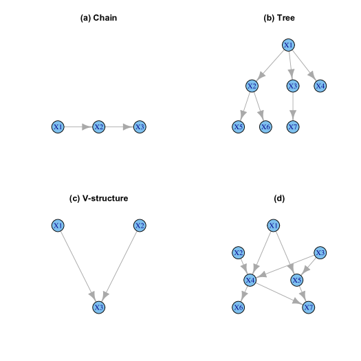
Figure 1: Four examples of Directed Acyclic Graph.

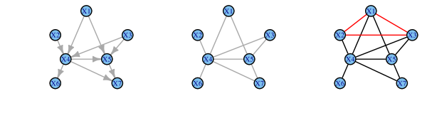
Figure 2: A DAG with seven nodes (left), its skeleton graph (middle) and its moral graph (right).

An important notion is d-separation.

Definition 1

A path from a node $x$ to another node $y$ is a sequence $x=\alpha_{0}\sim\alpha_{1}\sim\cdots\sim\alpha_{m}=y$. A path is said to be blocked by a subset of nodes $S$ if there exists a node on this path such that,

• either it is in the set $S$, and the arrows on the path do not meet head-to-head at this node, or

• neither the node, nor any of its descendants, is in the set $S$, and the arrows do meet head-to-head at this node.

(A node $x_{j}$ is called a descendant of another node $x_{i}$ if there is a directed path from $x_{i}$ to $x_{j}$ and $x_{i}$ is called an ancestor of $x_{j}$. )

Definition 2

Let $A,B,S$ be disjoint subsets of the node set $\mathbb{V}$. $A$ and $B$ are said to be d-separated by $S$ if all paths between $A$ and $B$ are blocked by $S$.

For the DAG in Figure 2, the set $S=(X_{4},X_{5})$ d-separates the sets $A=(X_{1},X_{2},X_{3})$ and $B=(X_{6},X_{7})$.

2.2 Factorization, I-map, P-map and I-equivalence

Next, we relate a probability distribution to a DAG which leads to the definition of DAG models. For each node $x_{i}$ of a DAG $\mathcal{G}$, we attach a random variable (also denoted by $x_{i}$) to it. We then consider a probability distribution $\mathbb{P}$ over the node set $\mathbb{V}=\{x_{1},\cdots,x_{p}\}$.

Definition 3

A distribution $\mathbb{P}$ is said to admit a recursive factorization (DF) according to a DAG $\mathcal{G}$ if it has a p.d.f. of the form:

$$p(\textbf{x})=\prod_{i=1}^{p}p(x_{i}|pa_{i}^{\mathcal{G}}),~{}~{}\textbf{x}=(x_{1},\cdots,x_{p})\in\mathcal{X},$$

where $p(x_{i}|pa_{i}^{\mathcal{G}})$ is the conditional probability density of $x_{i}$ given its parents $pa_{i}^{\mathcal{G}}$.

We can now formally define DAG models.

Definition 4

A DAG model is a pair $(\mathcal{G}(\mathbb{V},\mathbb{E}),\mathbb{P})$, where $\mathcal{G}$ is a DAG and $\mathbb{P}$ is a probability distribution over $\mathbb{V}$ which admits recursive factorization according to $\mathcal{G}$.

By definition, in a DAG model, the distribution $\mathbb{P}$ is specified by a set of local conditional probability distributions, namely, $\{p(x_{i}|pa_{i}^{\mathcal{G}}):i=1,\cdots,p\}$.

The factorization property leads to a compact representation of $\mathbb{P}$ if the graph $\mathcal{G}$ is sparse. In order to get a characterization of its independence properties, we need the notion of Markov property.

Definition 5

A distribution $\mathbb{P}$ is said to obey the directed global Markov property $(DG)$ according to a DAG $\mathcal{G}$ if whenever $A$ and $B$ are d-separated by $S$ in $\mathcal{G}$, there is $A$ and $B$ conditionally independent given $S$ under $\mathbb{P}$ , denoted by $A\mathchoice{\mathrel{\hbox to0.0pt{$\displaystyle\perp$\hss}\mkern 2.0mu{\displaystyle\perp}}}{\mathrel{\hbox to0.0pt{$\textstyle\perp$\hss}\mkern 2.0mu{\textstyle\perp}}}{\mathrel{\hbox to0.0pt{$\scriptstyle\perp$\hss}\mkern 2.0mu{\scriptstyle\perp}}}{\mathrel{\hbox to0.0pt{$\scriptscriptstyle\perp$\hss}\mkern 2.0mu{\scriptscriptstyle\perp}}}B|S~{}~{}~{}[\mathbb{P}]$.

It turns out that, DF and DG are equivalent [21].

Proposition 1

Let $\mathcal{G}$ be a DAG and $\mathbb{P}$ be a probability distribution over its node set which has a density with respect to a product measure $\mu$. Then $\mathbb{P}$ admits recursive factorization according to $\mathcal{G}$ if and only if $\mathbb{P}$ obeys directed global Markov property according to $\mathcal{G}$.

We can now try to characterize the independence properties of a distribution by a DAG. We need the notions of I-map and P-map.

Definition 6

Let $\mathcal{I}(\mathbb{P})$ denote all conditional independence assentations of the form $X_{A}\mathchoice{\mathrel{\hbox to0.0pt{$\displaystyle\perp$\hss}\mkern 2.0mu{\displaystyle\perp}}}{\mathrel{\hbox to0.0pt{$\textstyle\perp$\hss}\mkern 2.0mu{\textstyle\perp}}}{\mathrel{\hbox to0.0pt{$\scriptstyle\perp$\hss}\mkern 2.0mu{\scriptstyle\perp}}}{\mathrel{\hbox to0.0pt{$\scriptscriptstyle\perp$\hss}\mkern 2.0mu{\scriptscriptstyle\perp}}}X_{B}|X_{S}$ that hold under a distribution $\mathbb{P}$. Let $\mathcal{I}(\mathcal{G})$ be the set of conditional independence characterized by a DAG $\mathcal{G}$, i.e., $\mathcal{I}(\mathcal{G}):=\{X_{A}\mathchoice{\mathrel{\hbox to0.0pt{$\displaystyle\perp$\hss}\mkern 2.0mu{\displaystyle\perp}}}{\mathrel{\hbox to0.0pt{$\textstyle\perp$\hss}\mkern 2.0mu{\textstyle\perp}}}{\mathrel{\hbox to0.0pt{$\scriptstyle\perp$\hss}\mkern 2.0mu{\scriptstyle\perp}}}{\mathrel{\hbox to0.0pt{$\scriptscriptstyle\perp$\hss}\mkern 2.0mu{\scriptscriptstyle\perp}}}X_{B}|X_{S}:\hbox{$S$ d-separates $A$ and $B$ in $\mathcal{G}$}\}$. If $\mathcal{I}(\mathcal{G})\subseteq\mathcal{I}(\mathbb{P})$, then $\mathcal{G}$ is called an I-map of $\mathbb{P}$.

Proposition 1 says that, $\mathbb{P}$ factorizes according to $\mathcal{G}$ if and only if $\mathcal{G}$ is an I-map of $\mathbb{P}$. It is obvious that, the factorization property does not totally characterize the independence properties of a distribution. To see this, consider the distribution $\mathbb{P}$ under which $x_{i}$’s are mutually independent, then $\mathbb{P}$ factorizes according to any DAG (with nodes $x_{i}$’s). However, intuitively its “corresponding” DAG should be the empty graph. We thus have the following definition.

Definition 7

If $\mathcal{I}(\mathbb{P})=\mathcal{I}(\mathcal{G})$, i.e., all independencies in $\mathbb{P}$ are reflected by the d-separation properties in $\mathcal{G}$ and vice versa, then $\mathcal{G}$ is said to be a perfect map (P-Map) for $\mathbb{P}$.

Unfortunately, a P-map does not necessarily exist for a distribution $\mathbb{P}$. However, it can be shown that [19], for almost all distributions $\mathbb{P}$ that factorize over a DAG $\mathcal{G}$, we have $\mathcal{I}(\mathbb{P})=\mathcal{I}(\mathcal{G})$. On the other hand, there could be more than one P-maps for a distribution $\mathbb{P}$, as a set of independencies may be compatible to multiple DAGs.

Definition 8

Two DAGs $\mathcal{G}$ and $\tilde{\mathcal{G}}$ over the same set of nodes are said to be I-equivalent if $\mathcal{I}(\mathcal{G})=\mathcal{I}(\mathcal{\tilde{G}})$, i.e., they encode the same set of independencies.

We have the following characterization of I-equivalence [37].

Proposition 2

Two DAGs are I-equivalent if and only if they have the same set of skeleton edges and v-structures.

An immediate consequence of Proposition 2 is that I-equivalent DAGs have the same moral graph (but the converse is not true). The I-equivalent relation partitions the DAG space into equivalence classes. In the following, we use $\mathcal{E}(\mathcal{G})$ to denote the equivalence class that $\mathcal{G}$ belongs to.

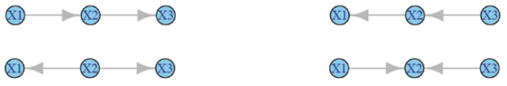
Figure 3: Four DAGs: $\mathcal{G}_{1}$ – upper left, $\mathcal{G}_{2}$ – upper right, $\mathcal{G}_{3}$– bottom left, $\mathcal{G}_{4}$ – bottom right.

In Figure 3, $\mathcal{G}_{1},\mathcal{G}_{2},\mathcal{G}_{3}$ are I-equivalent since they encode the same set of independencies: $\mathcal{I}=\{x_{1}\mathchoice{\mathrel{\hbox to0.0pt{$\displaystyle\perp$\hss}\mkern 2.0mu{\displaystyle\perp}}}{\mathrel{\hbox to0.0pt{$\textstyle\perp$\hss}\mkern 2.0mu{\textstyle\perp}}}{\mathrel{\hbox to0.0pt{$\scriptstyle\perp$\hss}\mkern 2.0mu{\scriptstyle\perp}}}{\mathrel{\hbox to0.0pt{$\scriptscriptstyle\perp$\hss}\mkern 2.0mu{\scriptscriptstyle\perp}}}x_{3}|x_{2}\}$, as in all three graphs, the only d-separation property is: $x_{2}$ d-separates $x_{1}$ from $x_{3}$. It is also clear that, they have the same moral graph: $x_{1}-x_{2}-x_{3}$. On the other hand, these three DAGs are not equivalent to $\mathcal{G}_{4}$ which has $\mathcal{I}=\{x_{1}\mathchoice{\mathrel{\hbox to0.0pt{$\displaystyle\perp$\hss}\mkern 2.0mu{\displaystyle\perp}}}{\mathrel{\hbox to0.0pt{$\textstyle\perp$\hss}\mkern 2.0mu{\textstyle\perp}}}{\mathrel{\hbox to0.0pt{$\scriptstyle\perp$\hss}\mkern 2.0mu{\scriptstyle\perp}}}{\mathrel{\hbox to0.0pt{$\scriptscriptstyle\perp$\hss}\mkern 2.0mu{\scriptscriptstyle\perp}}}x_{3}\}$ since in $\mathcal{G}_{4}$, $x_{1}$ and $x_{3}$ are de-separated by the empty set, but not by $x_{2}$. Its moral graph is $\begin{array}[]{ccc}x_{1}&-&x_{3}\\ \backslash&&/.\\ &x_{2}&\end{array}$

It is obvious that, it is impossible to distinguish I-equivalent DAGs based solely on the distribution $\mathbb{P}$. The best one can hope for is to learn the I-equivalence class corresponding to $\mathbb{P}$. Therefore, we formally define the goal of DAG structure learning as follows.

Definition 9

Given an i.i.d. sample $\mathbb{D}$ from a distribution $\mathbb{P}$, DAG structure learning is to recover the I-equivalence class of DAGs that are P-Maps for $\mathbb{P}$ (assuming existence of P-maps).

2.3 DAG structure learning

In this subsection, we give a brief overview of popular DAG structure learning methods. There are mainly three classes of methods for DAG learning, namely, score-based methods, constraint-based methods and hybrid methods.

In score-based methods, the DAG is viewed as specifying a model and structure learning is approached as a model selection problem. Specifically, a score-based method aims at minimizing a pre-specified score over the space of DAGs (defined on a given set of nodes). Commonly used scores include negative log-likelihood score, Akaike information criterion (AIC) score, Bayesian information criterion (BIC) score, Bayesian gaussian equivalent (BGe) score [13].

As mentioned earlier, the DAG space is super-exponentially large (with respect to the number of nodes) and thus an exhaustive search for models with the optimal score is usually infeasible. Therefore, greedy search algorithms are often employed. One of the most popular search algorithms for DAG learning is the hill climbing algorithm. At each search step, it conducts a local search among the graphs which are different from the current graph on a single edge [30]. Other options include conducting the search in the space of I-equivalence classes of DAGs [7] or using an ordering based algorithm [35].

In constraint-based methods, a DAG is viewed as a set of conditional independence constraints and the graph is learnt through conditional independence tests. One such method is the PC algorithm (PC-ALG) [37, 34, 17]. Other constraint-based methods include Grow and Shrink (GS) [23], Increament Association Markov Blanket (IAMB) and its two variants Fast IAMB and inter IAMB [39].

In hybrid methods, certain local structures of the graph such as the Markov blanket of each node are first learned, e.g., through independence tests and then such knowledge is used to impose restrictions on the search space in a score-based method. Hybrid methods include Max-Min Hill Climbing (MMHC) [36] and L1MB by [32].

In this paper, we focus on score-based methods. We first develop an efficient implementation of the hill climbing search algorithm (Section 3). We then propose aggregation strategies to improve the performance of DAG structure learning (Section 4). It should be noted that, the proposed aggregation procedure DAGBag can be coupled with any DAG learning algorithms whether it is score-based or constraint-based or hybrid.

3 An Efficient Structure Learning Algorithm

In this section, we first discuss decomposable scores used in score-based methods and the hill climbing algorithm for searching DAGs with the optimal score. We then propose an efficient implementation which greatly speeds up the hill climbing search algorithm and thus makes high-dimensional DAG structure learning computationally feasible.

3.1 Decomposable scores

In the rest of this paper, assume that we observe $n$ independently and identically distributed (i.i.d.) samples, $\mathbb{D}=\{X^{1},\cdots,X^{n}\}$, from a $p$-dimensional multivariate distribution $\mathbb{P}$ with mean $\boldsymbol{\mu}$ and covariance $\Sigma$, where $X^{k}=(x^{k}_{1},\cdots,x^{k}_{p})^{T}$ denotes the $k^{th}$ sample ($k=1,\cdots,n$). We also assume that the distribution $\mathbb{P}$ has a P-map. As mentioned earlier, our goal is to learn the I-equivalence class of DAGs which are P-maps of $\mathbb{P}$.

In the following, we use $X_{i}=\{x_{i}^{1},\cdots,x_{i}^{n}\}$ to denote the data of node $x_{i}$ ($i=1,\cdots,p$). Moreover, we use $\mathbb{G}(\mathbb{V})$ to denote the space of DAGs defined on the node set $\mathbb{V}=(x_{1},\cdots,x_{p})$. We first introduce the notion of decomposable scores.

Definition 10

A score defined on the DAG space $\mathbb{G}(\mathbb{V})$ is called decomposable if for any data $\mathbb{D}$ it has:

$$score(\mathcal{G}:\mathbb{D})=\sum^{p}_{i=1}score(x_{i}|pa^{\mathcal{G}}_{i}:\mathbb{D}),~{}~{}~{}\mathcal{G}\in\mathbb{G}(\mathbb{V}),$$

where $score_{i}:=score(x_{i}|pa^{\mathcal{G}}_{i}:\mathbb{D})$ only depends on the data of the node $x_{i}$ and the data of its parent set $pa^{\mathcal{G}}_{i}$ ($i=1,\cdots p$). Hereafter, we refer to $score_{i}$ as the neighborhood score of node $x_{i}$.

As we shall see in the next subsection, decomposable scores render efficient score updating in the search algorithm.

For the rest of this subsection, we adopt the working assumption that $\mathbb{P}$ is a multivariate normal distribution. We use $\theta$ to denote model parameters (in the Gaussian case, this includes the mean vector $\boldsymbol{\mu}$ and the covariance matrix $\Sigma$). Then for a given DAG $\mathcal{G}$, by the factorization property, the negative maximum-log-likelihood – the negative log-likelihood function evaluated at the restricted maximum likelihood estimator $\hat{\theta}_{\mathcal{G}}$ – leads to a decomposable score:

$$score_{like}(\mathcal{G}:\mathbb{D}) = -2\log\mathbb{P}_{\hat{\theta}_{\mathcal{G}}}(\mathbb{D})=\sum_{i=1}^{p}n\log(RSS_{i}/n),$$

where $RSS_{i}=RSS(x_{i}|pa^{\mathcal{G}}_{i}:\mathbb{D})$ is the residual sum of squares by least-squares regression of $x_{i}$ onto $pa_{i}^{\mathcal{G}}$ ($i=1,\cdots p$).

Structure learning based on the likelihood score will over-fit the data since it always favors larger models – distributions with less independence constraints which correspond to DAGs with more edges. Therefore, it is reasonable to consider scores that penalize for the model complexity. Two natural candidates are AIC and BIC which lead to the following decomposable scores:

$$score_{AIC}(\mathcal{G}:\mathbb{D}) = -2\log\mathbb{P}_{\hat{\theta}_{\mathcal{G}}}(\mathbb{D})+2|\mathbb{E}(\mathcal{G})|$$

$$= \sum_{i=1}^{p}\left(n\log(RSS_{i}/n)+2|pa_{i}^{\mathcal{G}}|\right),$$

where $|S|$ denotes the size of a set $S$, and

$$score_{BIC}(\mathcal{G}:\mathbb{D}) = -2\log\mathbb{P}_{\hat{\theta}_{\mathcal{G}}}(\mathbb{D})+|\mathbb{E}(\mathcal{G})|\log(n)$$

$$= \sum_{i=1}^{p}\left(n\log(RSS_{i}/n)+|pa_{i}^{\mathcal{G}}|\log(n)\right).$$

It can be shown that, $score_{BIC}$ is model selection consistent [6], meaning that as sample size $n$ goes to infinity (and the number of nodes $p$ being fixed), the following holds with probability going to one: (i) if $\mathcal{G}^{*}$ is a P-map of $\mathbb{P}$, then it will minimize the score; (ii) any $\mathcal{\tilde{G}}$ that is not a P-map of $\mathbb{P}$ will have a strictly larger BIC value. Furthermore, $score_{BIC}$ is also locally consistent [6], meaning that the following holds with probability going to one: (i) the score decreases by adding an edge that eliminates an independence constraint that is not implied by $\mathbb{P}$; (ii) the score increases by adding an edge that does not eliminate such a constraint. The local consistency property justifies the hill climbing search algorithm which conducts local updates of the model.

Under the Bayesian framework, various scores based on posterior probabilities of DAG have been proposed. These include the Bayesian Gaussian equivalent (BGe) score for multivariate normal distributions [13]. We will compare different scores in terms of their performance in DAG learning in Section 5.

3.2 Hill climbing algorithm

Given a score function, we want to find a DAG $\mathcal{G}^{\ast}$ that has the minimum score value among all DAGs, i.e.,

$$\mathcal{G}^{\ast}=\min_{\mathcal{G}\in\mathbb{G}(\mathbb{V})}score(\mathcal{G}:\mathbb{D}).$$

As mentioned earlier, due to the sheer size of the DAG space, an exhaustive search is infeasible for even moderate number of nodes. Therefore, heuristic search is often employed. A popular algorithm is the hill climbing algorithm which is a greedy iterative search algorithm. It starts with an empty graph (or an user given initial graph). At each subsequent step, a best operation, the one among the set of all eligible operations that results in the maximum reduction of the score, is used to update the current graph. The search stops when no operation is able to decrease the score anymore, which leads to a (local) optimal solution.

In the hill climbing algorithm for DAG learning, an operation is defined as either the addition of an absent edge, or the deletion of an existing edge, or the reversal of an existing edge. Moreover, an operation is eligible only if it does not result in cycles in the graph. This algorithm is outlined in Table 1.

Table 1: Hill climbing algorithm for DAG structure learning.

Input: data $\mathbb{D}$, node set $\mathbb{V}$, score function $score(\cdot:\cdot)$.

Initial step: $\mathcal{G}^{(0)}=$ empty graph; for $i=1,\cdots,p$, calculate $score_{i}(\mathcal{G}^{(0)}:\mathbb{D})$.

$s^{th}$ Step : Current graph $\mathcal{G}^{(s)}$.

$\bullet$ Acyclic check: for each potential operation, check whether applying it to $\mathcal{G}^{(s)}$ results in cycle or not.

$\bullet$ Score update: for each eligible operation $O$,

calculate the score change $\delta^{(s)}(O,\mathbb{D}):=score(O(\mathcal{G}^{(s)}):\mathbb{D})-score(\mathcal{G}^{(s)}:\mathbb{D})$,

where $O(\mathcal{G}^{(s)})$ denotes the graph resulting from applying $O$ to $\mathcal{G}^{(s)}$.

$\bullet$ Graph update: calculate $\delta^{(s)}_{\min}:=\min_{O}\delta^{(s)}(O,\mathbb{D})$.

$\bullet$ If $\delta^{(s)}_{\min}\geq 0$, stop the search algorithm and set $\mathcal{G}^{\ast}=\mathcal{G}^{(s)}$.

$\bullet$ Otherwise, choose the operation $O^{(s)}$ corresponding to $\delta^{(s)}_{\min}$.

$\bullet$ Set $\mathcal{G}^{(s+1)}=O^{(s)}(\mathcal{G}^{(s)})$.

$\bullet$ Proceed to step $s+1$.

Output: $\mathcal{G}^{\ast}$, the list of best operations $O^{(s)}$’s, the corresponding list of score decreases $\delta^{(s)}_{\min}$’s.

The major computational cost of the hill climbing algorithm is from the acyclic check for each potential operation (i.e., check whether the operation leads to cycles or not) and calculating score change for each eligible operation at every search step. Note that, by definition, an operation only results in the change in one (for addition and deletion operations) or two (for reversal operations) neighborhoods of the current graph. Consequently, for a decomposable score, an operation only changes the neighborhood score for up to two nodes. Therefore, the score updating step for each operation is computationally cheap as we only need to calculate the change of score for the neighborhood(s) involved in this operation. For instance, if operation $O$ is to add an edge $x_{i}\rightarrow x_{j}$, then applying $O$ on graph $\mathcal{G}$ leads to:

$$\delta(O,\mathbb{D})=score(O(\mathcal{G}):\mathbb{D})-score(\mathcal{G}:\mathbb{D})=score_{j}(O(\mathcal{G}):\mathbb{D})-score_{j}(\mathcal{G}:\mathbb{D}),$$

as only the neighborhood of $x_{j}$ is changed by operation $O$.

Nevertheless, even with decomposable scores, under the high-dimensional setting, acyclic check and score updating are costly due to the large number of potential operations ($\sim O(p^{2})$) at each search step. Moreover, when $p$ is large, it often takes many steps until the algorithm stops (i.e., to reach $\delta_{\min}\geq 0$). In the next subsection, we discuss efficient updating schemes which greatly speed up the search algorithm such that it may be used for high-dimensional DAG models learning.

3.3 Efficient score updating and acyclic check

In this subsection, we describe an efficient implementation of the hill climbing search algorithm for decomposable scores, where information from the previous step is re-used to facilitate both score updating and acyclic check in the current step.

We illustrate the idea by an example. Suppose the best operation selected in the previous step is to add $x_{i}\rightarrow x_{j}$. Then at the current step, the following holds: (i) any operation that does not involve neighborhood of $x_{j}$ results in the same score change as in the previous step; (ii) any operation that results in cycles in the previous step still leads to cycles; (iii) an operation that does not result in cycles in the previous step may only lead to cycles in the current step through $x_{i}\rightarrow x_{j}$. Therefore acyclic check can be performed very efficiently for such operations.

In the following, we use $\mathcal{\tilde{G}}$ to denote the graph in the previous step, $O^{\ast}$ to denote the selected operation by the previous step, and $\mathcal{G}^{\ast}=O^{\ast}(\mathcal{\tilde{G}})$ to denote the current graph. We also use $\delta(O:\mathcal{G})$ to denote the change of score resulting from applying operation $O$ to graph $\mathcal{G}$. We summarize the score updating and acyclic check schemes in the following two propositions.

Proposition 3

Suppose $score(\cdot:\cdot)$ is a decomposable score. For an (eligible) operation $O$, $\delta(O:\mathcal{\tilde{G}})=\delta(O:\mathcal{G}^{\ast})$, if one of the following holds:

• $O^{\ast}$ is one of the forms: “add $x_{i}\rightarrow x_{j}$” or “delete $x_{i}\rightarrow x_{j}$”, and $O$ is not one of the forms: “add $x_{k}\rightarrow x_{j}$” , “delete $x_{k}\rightarrow x_{j}$” , “ reverse $x_{j}\rightarrow x_{k}$ ”.

• $O^{\ast}$ is of the form “reverse $x_{i}\rightarrow x_{j}$”, and $O$ is not one of the forms: “add $x_{k}\rightarrow x_{j}$” , “delete $x_{k}\rightarrow x_{j}$” , “ reverse $x_{j}\rightarrow x_{k}$ ”, “add $x_{k}\rightarrow x_{i}$” , “delete $x_{k}\rightarrow x_{i}$”, “ reverse $x_{i}\rightarrow x_{k}$ ”.

In short, any operation that does not involve the neighborhoods changed by the selected operation in the previous step will lead to the same score change as in the previous step. This has been pointed out by [19].

In the following, $de(x_{i})$ denotes the set of descendent of node $x_{i}$ and $an(x_{i})$ denotes the set of ancestors of node $x_{i}$.

Proposition 4

The following holds for acyclic check.

• If $O^{\ast}$ is of the form “add $x_{i^{\ast}}\rightarrow x_{j^{\ast}}$”, then for an operation $O$ the following holds:

  • If $O$ does not lead to cycles in the previous step, then

    • if $O$ is of the form “add $x_{i}\rightarrow x_{j}$”, and $i\in de(x_{j^{\ast}})$ and $j\in an(x_{i^{\ast}})$, then $O$ leads to a cycle.

    • if $O$ is of the form “reverse $x_{i}\rightarrow x_{j}$”, and $j\in de(x_{j^{\ast}})$ and $i\in an(x_{i^{\ast}})$, then $O$ leads to a cycle.

    • if otherwise, $O$ remains acyclic.

  • If $O$ leads to a cycle in the previous step, it remains cyclic.

• If $O^{\ast}$ is of the form “delete $x_{i^{\ast}}\rightarrow x_{j^{\ast}}$”, then for an operation $O$ the following holds:

  • If $O$ does not lead to cycles in the previous step, it remains acyclic.

  • If $O$ leads to a cycle in the previous step, then

    • if $O$ is of the form “add $x_{i}\rightarrow x_{j}$”, and $i\in de(x_{j^{\ast}})$ and $j\in an(x_{i^{\ast}})$, then we need to check its acyclicity;

    • if $O$ is of the form “reverse $x_{i}\rightarrow x_{j}$”, and $j\in de(x_{j^{\ast}})$ and $i\in an(x_{i^{\ast}})$, then we need to check its acyclicity;

    • if otherwise, $O$ remains cyclic.

• If $O^{\ast}$ is of the form “reverse $x_{i^{\ast}}\rightarrow x_{j^{\ast}}$”, then for an operation $O$ the following holds:

  • If $O$ does not lead to cycles in the previous step, then

    • if $O$ is of the form “add $x_{i}\rightarrow x_{j}$”, and $i\in de(x_{i^{\ast}})$ and $j\in an(x_{j^{\ast}})$, then $O$ leads to a cycle.

    • if $O$ is of the form “reverse $x_{i}\rightarrow x_{j}$”, and $j\in de(x_{i^{\ast}})$ and $i\in an(x_{j^{\ast}})$, then $O$ leads to a cycle.

    • if otherwise, $O$ remains acyclic.

  • If $O$ leads to a cycle in the previous step, then

    • if $O$ is of the form “add $x_{i}\rightarrow x_{j}$”, and $i\in de(x_{j^{\ast}})$ and $j\in an(x_{i^{\ast}})$, then we need to check its acyclicity;

    • if $O$ is of the form “reverse $x_{i}\rightarrow x_{j}$”, and $j\in de(x_{j^{\ast}})$ and $i\in an(x_{i^{\ast}})$, then we need to check its acyclicity;

    • if otherwise, $O$ remains cyclic.

It is clear from the above two propositions that at each search step, only for a fraction of operations we need to calculate their score change and check the acyclic status. For the majority of operations, score change and acyclic status remain the same as those in the previous step and thus do not need to be re-assessed.

The implementation with these efficient updating schemes greatly speeds up the search algorithm. For example, for a graph with $p=1000$ nodes, sample size $n=250$, conducting $2000$ search steps takes $\sim 150$ seconds under our implementation and $\sim 2,500$ seconds under the hc function in bnlearn R package [33] (version 3.3, published on 2013-03-05). The above numbers are user times averaged over $10$ simulation replicates performed on a machine with 8GB memory and 2quad CPU.

We defer additional implementation details including early stopping and random restart into the Appendix (Section A-0.1).

4 Bootstrap Aggregating for DAG Learning

In this section, we propose the DAGBag procedure which is inspired by bootstrap aggregating – Bagging [3]. Bagging is originally proposed to get an aggregated prediction rule based on multiple versions of prediction rules built on bootstrap resamples of the data. It is most effective in improving highly variable learning procedures such as classification trees through variance reduction. Recently, the aggregation idea has been applied to learn stable structures in high-dimensional regression models and Gaussian graphical models [24, 38, 22].

4.1 DAGBag

As with many structure learning procedures, DAG learning procedures are usually highly variable – the learned graph changes drastically with even small perturbation of the data. Therefore, we propose to utilize the aggregation idea in DAG learning to search for stable structures. In particular, through aggregation we are able to alleviate over-fitting and greatly reduce the number of false positive edges.

In DAGbag, an ensemble of DAGs $\mathbb{G}^{e}=\{\mathcal{G}_{b}\}_{b=1}^{B}$ are first learned based on bootstrap resamples $\{\mathbb{D}_{b}\}_{b=1}^{B}$ of the original data $\mathbb{D}$ by a DAG learning procedure, e.g., a score-based method. Then an aggregated DAG is learned based on this ensemble. Aggregation of a collection of DAGs is nontrivial because the notion of average is not straightforward on the DAG space. Here, we generalize the idea of median by searching for a DAG that minimizes an average distance to the DAGs in the ensemble:

$$\mathcal{G}^{*}={\rm argmin}_{\mathcal{G}\in\mathbb{G}(\mathbb{V})}score_{d}(\mathcal{G}:\mathbb{G}^{e}),$$

where

$$score_{d}(\mathcal{G}:\mathbb{G}^{e}):=\frac{1}{B}\sum^{B}_{b=1}d(\mathcal{G},\mathcal{G}_{b})$$

with $d(\cdot,\cdot)$ being a distance matric on the DAG space. As a general recipe, the aggregated DAG $\mathcal{G}^{\ast}$ may be learned by the hill climbing search algorithm. However, as shown in the next subsection, for the family of distance metrics based on the structural hamming distance, the search can be conducted in a much more efficient manner.

The DAGBag procedure is outlined in Table 2.

Table 2: DAGBag procedure.

Input: data $\mathbb{D}$, node set $\mathbb{V}$, DAG learning procedure $\mathcal{L}$, distance measure $d(\cdot,\cdot)$ on the DAG space $\mathbb{G}(\mathbb{V})$,

number of bootstrap samples $B$.

Bootstrapping: obtain $B$ bootstrap samples of the data: $\mathbb{D}_{1},\cdots,\mathbb{D}_{B}$.

Ensemble of DAGs: for $b=1,\cdots,B$, learn a DAG $\mathcal{G}_{b}$ based on resample $\mathbb{D}_{b}$ by learning procedure $\mathcal{L}$.

Obtain an ensemble of DAGs: $\mathbb{G}^{e}:=\{\mathcal{G}_{1},\cdots,\mathcal{G}_{B}\}$.

Aggregation: learn an aggregated DAG:

$\mathcal{G}^{*}={\rm argmin}_{\mathcal{G}\in\mathbb{G}(\mathbb{V})}score_{d}(\mathcal{G}:\mathbb{G}^{e})$, where $score_{d}(\mathcal{G}:\mathbb{G}^{e}):=\frac{1}{B}\sum^{B}_{b=1}d(\mathcal{G},\mathcal{G}_{b})$.

Output: aggregated DAG $\mathcal{G}^{*}$.

4.2 Structural Hamming distances and aggregation scores

One crucial aspect of the DAGBag procedure is the distance metric $d(\cdot,\cdot)$ on DAG space which dictates how the ensemble of DAGs should be aggregated. In this subsection, we discuss distance metrics based on the structural Hamming distance (SHD) and the properties of their corresponding aggregation scores.

In information theory, the Hamming distance between two 0-1 vectors of equal length is the minimum number of substitutions needed to convert one vector to another. This can be generalized to give a distance measure between DAGs with the same set of nodes.

Definition 11

A structural Hamming distance between $\mathcal{G},\mathcal{\tilde{G}}\in\mathbb{G}(\mathbb{V})$ is defined as :

$$d(\mathcal{G},\mathcal{\tilde{G}}):=\text{the minimum number of operations needed to covert $\mathcal{G}$ to $\mathcal{\tilde{G}}$.}$$

It is obvious that, this definition leads to valid distance measures as: (i) $d(\mathcal{G},\mathcal{\tilde{G}})\geq 0$, “$=0$” if and only if $\mathcal{G}=\mathcal{\tilde{G}}$; (ii) $d(\mathcal{G},\mathcal{\tilde{G}})=d(\mathcal{\tilde{G}},\mathcal{G})$; (iii) $d(\mathcal{G},\mathcal{\tilde{G}})\leq d(\mathcal{G},\mathcal{G}^{\ast})+d(\mathcal{G}^{\ast},\mathcal{\tilde{G}})$.

As in the hill climbing search algorithm, we may define an operation as, the addition of an absent edge, or the deletion of an existing edge, or the reversal of an existing edge, which does not lead to cycles. In this subsection, we propose variants of SHD on DAG space where the difference among these variants lies in how reversal operations are counted.

Specifically, the addition or the deletion of an edge is always counted as one unit of operation. If the reversal of an edge is counted as two units of operations, then we have the following distance measure:

$$d_{SHD}(\mathcal{G},\mathcal{\tilde{G}}) = \sum_{i=1}^{p}\sum_{j=1}^{p}|\mathbb{A}(i,j)-\mathbb{\tilde{A}}(i,j)|=\sum_{1\leq i<j\leq p}|\mathbb{A}(i,j)-\mathbb{\tilde{A}}(i,j)|+|\mathbb{A}(j,i)-\mathbb{\tilde{A}}(j,i)|,$$

$$= \sum_{i=1}^{p}\sum_{j=1}^{p}\left(\mathbb{A}(i,j)-\mathbb{\tilde{A}}(i,j)\right)^{2},$$

where $\mathbb{A},\mathbb{\tilde{A}}$ denote the adjacency matrices of $\mathcal{G}$ and $\mathcal{\tilde{G}}$, respectively. Note that $d_{SHD}(\mathcal{G},\mathcal{\tilde{G}})$ is both the $\ell_{1}$ distance and the $\ell_{2}$ distance between the two adjacency matrices.

If the reversal of an edge is also counted as one unit of operation, then we have the following distance measure:

$$d_{adjSHD}(\mathcal{G},\mathcal{\tilde{G}})=\sum_{1\leq i<j\leq p}\max\{|\mathbb{A}(i,j)-\mathbb{\tilde{A}}(i,j)|,|\mathbb{A}(j,i)-\mathbb{\tilde{A}}(j,i)|\}.$$

More generally, one may count the reversal of an edge as $\alpha(>0)$ units of operations which leads to the following family of distances.

Definition 12

For $\alpha>0$, the generalized structural Hamming distance $d_{GSHD(\alpha)}$ on the DAG space $\mathbb{G}(\mathbb{V})$ is defined as:

$$d_{GSHD(\alpha)}(\mathcal{G},\mathcal{\tilde{G}})=\sum_{1\leq i<j\leq p}S_{ij}(\mathbb{A},\mathbb{\tilde{A}};\alpha),~{}~{}\mathcal{G},\mathcal{\tilde{G}}\in\mathbb{G}(\mathbb{V}),$$

where $S_{ij}(\mathbb{A},\mathbb{\tilde{A}};\alpha)$ is defined as following:

• If $|\mathbb{A}(i,j)-\mathbb{\tilde{A}}(i,j)|+|\mathbb{A}(j,i)-\mathbb{\tilde{A}}(j,i)|=0$, then $S_{ij}(\mathbb{A},\mathbb{\tilde{A}};\alpha)=0$;

• If $|\mathbb{A}(i,j)-\mathbb{\tilde{A}}(i,j)|+|\mathbb{A}(j,i)-\mathbb{\tilde{A}}(j,i)|=1$, then $S_{ij}(\mathbb{A},\mathbb{\tilde{A}};\alpha)=1$;

• If $|\mathbb{A}(i,j)-\mathbb{\tilde{A}}(i,j)|+|\mathbb{A}(j,i)-\mathbb{\tilde{A}}(j,i)|=2$, then $S_{ij}(\mathbb{A},\mathbb{\tilde{A}};\alpha)=\alpha$.

It is easy to see that, $d_{SHD}$ corresponds to $\alpha=2$ and $d_{adjSHD}$ corresponds to $\alpha=1$. In the literature, $d_{SHD}$ and $d_{GSHD(0.5)}$ have been used to compare a learned DAG to the “true” DAG as performance evaluation criteria of DAG learning procedures in numerical studies [36, 28].

In $d_{SHD}$, a reversely oriented direction is penalized twice as much as a missing or an extra skeleton edge. Since edge directions are not always identifiable, it is reasonable to penalize a reversely oriented direction less severely. This is supported by our numerical results where aggregation based on $d_{adjSHD}$ (or $d_{GSHD(\alpha)}$ with an $\alpha<2$) usually outperforms aggregation based on $d_{SHD}$. In general, with larger $\alpha$, the aggregated DAG retains less edges and tends to have smaller false positive edges as well as less correct edges.

In the following, we use score.SHD, score.adjSHD and score.GSHD$(\alpha)$ to denote aggregation scores based on $d_{SHD}$, $d_{adjSHD}$ and $d_{GSHD(\alpha)}$, respectively.

In Proposition 5 below, we derive an expression of score.SHD in terms of edge selection frequencies (SF).

Definition 13

Given an ensemble of DAGs: $\mathbb{G}^{e}=\{\mathcal{G}_{b}:b=1,\cdots B\}$, the selection frequency (SF) of a directed edge $e$ is defined as

$$p_{e}:=\#\{\mathcal{G}_{b}:e\in\mathbb{E}(\mathcal{G}_{b})\}/B,$$

where $\mathbb{E}(\mathcal{G}_{b})$ denotes the edge set of DAG $\mathcal{G}_{b}$.

Proposition 5

Given an ensemble of DAGs: $\mathbb{G}^{e}=\{\mathcal{G}_{b}:b=1,\cdots B\}$, the aggregation score under $d_{SHD}$ is

$$score.SHD(\mathcal{G}:\mathbb{G}^{e})=\sum_{e\in\mathbb{E}(\mathcal{G})}(1-2p_{e})+C,$$

where

$$C=\frac{1}{B}\sum_{b=1}^{B}\sum_{i=1}^{p}\sum_{j=1}^{p}\mathbb{A}_{b}(i,j)=\sum_{i=1}^{p}\sum_{j=1}^{p}p_{x_{i}\rightarrow x_{j}},$$

is a constant which only depends on the ensemble $\mathbb{G}^{e}$, but does not depend on $\mathcal{G}$.

By Proposition 5, $score.SHD$ is super-decomposable in that it is an additive function of the selection frequencies of individual edges. Moreover, the DAG $\mathcal{G}^{\ast}$ that minimizes score.SHD could only contain edges with selection frequency larger than $50\%$ and it should contain as many such edges as possible. Indeed, as shown by Proposition 6, the hill climbing algorithm is simplified to the algorithm described in Table 3.

Table 3: Hill climbing algorithm with aggregation score.SHD.

Input: an ensemble of DAGs: $\mathbb{G}^{e}=\{\mathcal{G}_{b}:b=1,\cdots B\}$.

Calculate selection frequency for all possible edges.

Order edges with selection frequency $>50\%$.

Add edges sequentially according to SF and stop when SF $\leq 0.5$.

$\bullet$ Initial step: $\mathcal{G}^{(0)}$= empty graph, $\mathbb{C}=$ empty set.

$\bullet s^{th}$ step: current graph $\mathcal{G}^{(s)}$, current operation $O$: “add the edge with the $s^{th}$ largest SF”.

$\bullet$ If $O$ passes the acyclic check, then $\mathcal{G}^{(s+1)}=O(\mathcal{G}^{(s)})$, i.e., add this edge.

If $O$ does not pass the acyclic check, then $\mathcal{G}^{(s+1)}=\mathcal{G}^{(s)}$, i.e., does not add this edge,

and add this edge to $\mathbb{C}$.

$\bullet$ If the $(s+1)^{th}$ largest SF $>50\%$, proceed to step $s+1$.

Otherwise, set $\mathcal{G}^{\ast}=\mathcal{G}^{(s+1)}$ and stop the algorithm.

Output: $\mathcal{G}^{\ast}$, and the set of “cyclic edges” $\mathbb{C}$.

Proposition 6

In each step of the hill climbing algorithm with score.SHD, the following operations (assuming eligible) will not decrease the score:

• add an edge with selection frequency $\leq 0.5$;

• delete an edge in the current graph;

• reverse an edge in the current graph.

Moreover, among eligible edge addition operations, the one corresponding to the largest selection frequency will lead to the most decrease of score.SHD. Therefore, the hill climbing search algorithm can be conducted as described in Table 3.

In addition, it is shown in Proposition 7 that, the algorithm in Table 3 leads to a global optimal solution if the set of “cyclic edges” $\mathbb{C}$ (defined in Table 3) has at most one edge.

Proposition 7

Given an ensemble of DAGs: $\mathbb{G}^{e}=\{\mathcal{G}_{b}:b=1,\cdots B\}$ defined on node set $\mathbb{V}$, the DAG $\mathcal{G}^{\ast}$ obtained by the algorithm in Table 3 reaches the minimum score.SHD value:

$$score.SHD(\mathcal{G}^{\ast}:\mathbb{G}^{e})=\min_{\mathcal{G}\in\mathbb{G}(\mathbb{V})}score.SHD(\mathcal{G}:\mathbb{G}^{e}),$$

provided that $|\mathbb{C}|\leq 1$.

The proofs of Propositions 5, 6 and 7 are given in the Appendix (A-0.2).

All the above results for score.SHD can be generalized to score.GSHD$(\alpha)$. For this purpose, we need the definition of generalized selection frequency.

Definition 14

Given an ensemble of DAGs: $\mathbb{G}^{e}=\{\mathcal{G}_{b}:b=1,\cdots B\}$ and an $\alpha>0$, the generalized selection frequency (GSF) of a directed edge $e$ is defined as

$$gp_{e}(\alpha):=p_{e}+(1-\frac{\alpha}{2})p_{e^{*}},$$

where $e^{*}$ denotes the edge with the reversed direction of $e$.

score.GSHD can be expressed in terms of generalized selection frequencies.

Proposition 8

Given an ensemble of DAGs: $\mathbb{G}^{e}=\{\mathcal{G}_{b}:b=1,\cdots B\}$ and an $\alpha>0$, the aggregation score under $d_{GSHD(\alpha)}$ is

$$score.GSHD(\alpha)(\mathcal{G}:\mathbb{G}^{e})=\sum_{e\in\mathbb{E}(\mathcal{G})}(1-2gp_{e}(\alpha))+C,$$

where

$$C=\frac{1}{B}\sum_{b=1}^{B}\sum_{i=1}^{p}\sum_{j=1}^{p}\mathbb{A}_{b}(i,j)=\sum_{i=1}^{p}\sum_{j=1}^{p}p_{x_{i}\rightarrow x_{j}},$$

is a constant which only depends on the ensemble $\mathbb{G}^{e}$, but does not depend on $\mathcal{G}$.

Also the hill climbing search algorithm with score.GSHD can be simplified to the procedure described in Table 4 (Proposition 9). Note that, only when $\alpha=2$, the GSF of an edge $e$ does not depend on the SF of the reversed edge $e^{*}$, and the search under the corresponding score score.SHD only depends on the SF of individual edges. For $\alpha$ other than $2$, the search depends on the SF of pairs of reversely oriented edges through GSF. In particular, the larger $\alpha$ is, the more an edge would be penalized by the extent of how frequently the reversed edge appeared in the ensemble.

Table 4: Hill climbing algorithm with aggregation score.GSHD$(\alpha)$.

Input: an ensemble of DAGs: $\mathbb{G}^{e}=\{\mathcal{G}_{b}:b=1,\cdots B\}$, an $\alpha>0$.

Calculate generalized selection frequency $gp_{e}(\alpha)$ for all possible edges.

Order edges with generalized selection frequency $>50\%$.

Add edges sequentially according to GSF and stop when GSF $\leq 0.5$.

$\bullet$ Initial step: $\mathcal{G}^{(0)}$= empty graph, $\mathbb{C}=$ empty set.

$\bullet s^{th}$ step: current graph $\mathcal{G}^{(s)}$, current operation $O$: “add the edge with the $s^{th}$ largest GSF”.

$\bullet$ If $O$ passes the acyclic check, then $\mathcal{G}^{(s+1)}=O(\mathcal{G}^{(s)})$, i.e., add this edge.

If $O$ does not pass the acyclic check, then $\mathcal{G}^{(s+1)}=\mathcal{G}^{(s)}$, i.e., does not add this edge,

and add this edge to $\mathbb{C}$.

$\bullet$ If the $(s+1)^{th}$ largest GSF $>50\%$, proceed to step $s+1$.

Otherwise, set $\mathcal{G}^{\ast}=\mathcal{G}^{(s+1)}$ and stop the algorithm.

Output: $\mathcal{G}^{\ast}$, and the set of “cyclic edges” $\mathbb{C}$.

Proposition 9

In each step of the hill climbing algorithm with score.GSHD$(\alpha)$, the following operations (assuming eligible) will not decrease the score:

• add an edge with generalized selection frequency $\leq 0.5$;

• delete an edge in the current graph;

• reverse an edge in the current graph.

Moreover, among eligible edge addition operations, the one corresponding to the largest generalized selection frequency will lead to the most reduction of score.GSHD$(\alpha)$. Therefore, the hill climbing search algorithm can be conducted as described in Table 4.

In addition, $\mathcal{G}^{\ast}$ reaches the minimum score.GSHD$(\alpha)$ value:

$$score.GSHD(\alpha)(\mathcal{G}^{\ast}:\mathbb{G}^{e})=\min_{\mathcal{G}\in\mathbb{G}(\mathbb{V})}score.GSHD(\alpha)(\mathcal{G}:\mathbb{G}^{e}),$$

provided that $|\mathbb{C}|\leq 1$.

The proofs of Propositions 8 and 9 are given in the Appendix (Section A-0.2).

5 Numerical Study

In this section, we conduct an extensive simulation study to examine the proposed DAGBag procedure and compare it to several existing DAG learning algorithms.

5.1 Simulation setting

Given the true data generating DAG $\mathcal{G}$ and a sample size $n$, $n$ i.i.d. samples are generated according to the Gaussian linear mechanism corresponding to $\mathcal{G}$:

$$x_{i}=\sum_{j\in pa_{i}^{\mathcal{G}}}\beta_{ij}x_{j}+\epsilon_{i},~{}~{}~{}i=1,\cdots,p,$$

where $\epsilon_{i}$s are independent Gaussian random variables with mean zero and variance $\sigma^{2}_{i}$.

The coefficients $\beta_{ij}$s in the linear mechanism are uniformly generated from $\mathcal{B}=[-0.5,-0.3]\cup[0.3,0.5]$. The error variances $\sigma^{2}_{i}$s are chosen such that for each node the corresponding signal-to-noise-ratio (SNR), defined as the ratio between the standard deviation of the signal part and that of the noise part, is in a given range $\mathcal{R}$. Here we consider two settings, namely, a high SNR case $\mathcal{R}=[0.5,1.5]$ and a low SNR case $\mathcal{R}=[0.2,0.5]$.

The generated data are standardized to have sample mean zero and sample variance one before applying any DAG structure learning algorithm. For DAGBag, the number of bootstrap resamples is set to be $B=100$ and the learning algorithm applied to each resample is the score-based method with BIC score. For each simulation setting, $100$ independent replicates are generated.

We consider DAGs with different dimension and complexity as well as different sample sizes. The data generating graphs are shown in Figures B-1 to B-6 in the Appendix (Section B-1). Statistics of each graph and the simulation parameters are given in Table 5.

Table 5: Graph statistics and simulation parameters.

DAG	$p$	$|\mathbb{E}|$	V-struct	Moral $|\mathbb{E}|$	$n$	SNR	max-step∗
Empty Graph	1000	0	0	0	250	[0.5,1.5]	2000
Tree Graph	100	99	0	99	50	[0.5,1.5]	500
					50,102,	[0.2,0.5]
Sparse Graph	102	109	77	184	200, 500,	[0.5,1.5]	500
					1000, 5000
Dense Graph	104	527	1675	1670	100	[0.2,0.5]	1000
						[0.5,1.5]
Large Graph	504	515	307	808	100, 250	[0.2,0.5]	1000
						[0.5,1.5]
Extra-Large Graph	1000	1068	785	1823	100, 250	[0.5,1.5]	5000
Ultra-Large Graph	2639	2603	1899	4481	250	[0.5,1.5]	10000

^∗ maximum number of steps allowed in the search algorithm.

5.2 Performance evaluation

We report results on skeleton edge, v-structure and moral edge (edges in the moral graph) detection by tables and figures. The reason to report results on these objects is because they are identifiable: I-equivalent DAGs have same sets of skeleton edges, v-structures and moral edges.

In the tables in Appendix C-1, for each method, the numbers of skeleton edges, v-structures and moral edges of the learned graph, denoted by “Total E”, “Total V” and “Total M”, as well as the numbers of correctly identified skeleton edges, correctly identified v-structures and correctly identified moral edges, denoted by “Correct E”, “Correct V”, “Correct M”, are reported. All numbers are averaged over the results on $100$ replicates. The standard deviations are given in the parenthesis.

Under a given setting, if the learned graph of one method has similar or less number of edges than the learned graph of another method, while at the same time it identifies more correct edges, then it is fair to say that this method outperforms the other one because of less false positives and higher power. However, quite often, the method with less number of edges also identifies less correct edges, making methods comparison difficult. Therefore, besides recording the results at the learned graphs, we also draw learning curves for edge/v-structure detection to facilitate methods comparison.

For methods using a search algorithm, at each search step, we record the number of skeleton edges (v-structures) and the number of correct skeleton edges (v-structures) of the current graph. We then draw a “Total E” (“Total V”) versus “Correct E” (“Correct V”) curve across search steps. The end point of each curve denotes the result of the leaned graph (i.e., the place at which the search algorithm stops). For MMHC (by R package bnlearn) and PC-Alg (by R package pcalg), there is a tuning parameter $\alpha$ denoting the significance level used by the independence tests. Therefore, their learning curves are driven by this parameter: we run the algorithm on a series of $\alpha$ and draw the learning trajectory based on results across $\alpha$’s.

If the learning curve of one method lies above that of another method, then the former method is better among the two, since it detects more correct edges (v-structures) at each given number of total edges (v-structures).

5.3 Results and findings

False positive reduction by aggregation

To illustrate the effectiveness of the aggregation methods in false positive reduction, we first consider an empty graph with $p=1000$ nodes, $|\mathbb{E}|=0$ edge and sample size $n=250$. As can been seen from Table C-1, aggregation methods result in very few false positive edges, whereas the non-aggregation methods, namely, score, MMHC and PC-Alg, all have very large number of false positives. Same patterns are observed on the same graph with a larger sample size $n=500$ (results omitted).

We then consider a graph with $p=504$ nodes, $|\mathbb{E}|=515$ edges and $|\mathbb{VS}|=307$ v-structures (Figure B-4), under two sample sizes, $n=100$ and $n=250$, with $SNR\in[0.5,1.5]$. Figures B-7 and B-8 show the learning curves (driven by the updating steps in the search algorithm) in terms of skeleton edge detection and v-structure detection. The end point of each curve indicates the place where the corresponding algorithm stops (i.e., the learned graph). For the purpose of a better graphical presentation, the curves corresponding to score are cut short (since it stops much later than other methods) with the corresponding numbers given in the caption. Tables C-10 and C-11 in Appendix C-1 show the total number of skeleton edges/v-structures and correct number of skeleton edges/v-structures in the learned graph by each method.

As can be seen from these figures, the aggregation methods have learning curves (colored curves) well above those of the non-aggregation score method (black curves) in both skeleton edge detection and v-structure detection, demonstrating their superior performance. Moreover, aggregation methods stop much earlier than the score method due to the (implicit) model regularization resulted from aggregation. This is why aggregation methods have much reduced number of false positives.

Among score.GSHD$(\alpha)$ methods, adjSHD ($\alpha=1$), GSHD$(0.5)$ and GSHD$(1.5)$ have very similar learning curves, with the ones with smaller $\alpha$ stop later (i.e., more edges, higher false positive rate and higher power). SHD ($\alpha=2$) has inferior learning curves in edge detection and slightly better learning curves in v-structure detection compared with other score.GSHD methods with smaller $\alpha$. It also stops much earlier, demonstrating that over-penalization of edge direction discrepancy is detrimental for both learning efficiency (represented by learning curves) and power (represented by the position of the end point).

We also consider a Tree Graph with $p=100$ nodes (Figure B-1), where we compare the aggregation based methods with the minimum spanning tree (MST) algorithm [20, 29]. MST is the method of choice if we know aprior that the graph is a tree. When sample size is $n=50$ (Table C-2), the aggregation methods have less power than MST, but their false positive rates remain low. When sample size is increased to $n=100$ (results omitted), the aggregation methods are able to achieve a performance similar to that of MST.

Other main observations are listed below. More detailed results can be found in Appendix B-1 (learning curves) and Appendix C-1 (tables).

• For the high SNR setting $(SNR\in[0.5,1.5])$, aggregation methods have superior learning curves compared to the non-aggregating methods, in both skeleton edge detection and v-structure detection.

• For the low SNR setting $(SNR\in[0.2,0.5])$, under Sparse Graph (Figure B-2) and Dense Graph (Figure B-3) (both graphs have $p\sim 100$) with $n\sim 100$, all methods tend to have similar learning curves in terms of skeleton edge detection and all of them perform poorly in v-structure detection due to lack of power (thus corresponding learning curves are not shown). While under the Large Graph ($p\sim 500$), the aggregation methods have better learning curves for both SNR ranges under both $n=100$ and $n=250$.

• For all settings, aggregation based methods stop much earlier than the non-aggregation score method. This is due to model regularization induced by the aggregation process and it leads to much reduced number of false positives.

• In terms of skeleton edge detection, adjSHD, GSHD(1.5),GSHD(0.5) have superior learning curves compared to SHD. The differences are more pronounced in the high SNR cases.

• In terms of v-structure detection, all aggregation based methods have somewhat similar learning curves. The main difference among these methods lie in where the search algorithm stops.

In summary, aggregation based methods are particularly competitive for either high SNR or high-dimensional settings.

Effect of sample size on aggregation methods

Here we study effect of sample size on DAG learning procedures. By comparing results on Large Graph with both SNR ranges: $n=100$ vs. $n=250$ (Table C-10 vs. Table C-11; Table C-12 vs. Table C-13), it appears that sample size $n$ does not have much effect on the false positive rate of the aggregation methods. Even under small sample sizes, the aggregation methods are able to maintain a low false positive rate. The effect of sample size is mainly in power: the smaller $n$, the less power in edge/v-structure detection.

Due to the consistency of the BIC score, we expect all methods (including score) will converge to a graph in the true I-equivalence class when $n$ goes to infinity. We conduct a simulation on Spare Graph with $SNR\in[0.5,1.5]$ under a series of sample sizes $n=50,102,200,500,1000,5000$ to demonstrate such a convergence. Figure B-13 shows the skeleton edge detection learning curves of score and adjSHD under different sample sizes. It can be seen that, the curves corresponding to larger sample sizes lie above those corresponding to smaller sample sizes. Moreover, with $n$ increasing, the curves become closer to the diagonal line where number of false positives becomes zero. These results are also given in Table C-6.

Effect of graph topology on aggregation methods

Here we study the effect of graph topology on aggregation methods (focusing on adjSHD for ease of comparison and illustration). We first compare the results under the Sparse Graph which has $p\sim 100,|\mathbb{E}|\sim 100$ (Figure B-2) to the results under the Dense Graph which has $p\sim 100,|\mathbb{E}|\sim 500$ and many more v-structures (Figure B-3). For simulations with $n\sim 100$ and $SNR\in[0.5,1.5]$ (Table C-3 vs. Table C-8), the power is much smaller under the Dense Graph due to its higher intrinsic dimension/more complex model. However, the false positive rate is only slightly higher under the Dense Graph. This again demonstrates the effectiveness of the aggregation methods in false positive reduction even when the underlying model is complex.

We then compare the results under Large ($p\sim 500$, Figure B-4), Extra-large ($p\sim 1000$, Figure B-5) and Ultra-large ($p\sim 2600$, Figure B-6) graphs. All these graphs have similar edge/node ratio in that $p\sim|\mathbb{E}|$. However they have increasing number of nodes. For simulations with $n=250$ and $SNR\in[0.5,1.5]$ (Tables C-11, C-15,C-16), both false positive rates and powers are quite similar across these three networks. This indicates that, the nominal dimension alone does not have much effect on performance of aggregation methods.

In summary, for aggregation methods, false positive rate is not much affected by the complexity of the underlying model, while the power is lower for more complex models. Moreover, the complexity of the model is not much affected by the nominal dimension (i.e., the number of nodes), but rather factors including the intrinsic dimension, degree of sparsity of the network, the number of v-structures, etc.

Robustness to distributional assumptions

To investigate the robustness of the score-based procedures (aggregation or not) to the Normality assumption, instead of sampling the residual terms of the linear mechanisms from Normal distributions, they are sampled from mean-centered student t-distributions (df $=3$ and df $=5$) and Gamma distributions (shape parameter $=1$, scale parameter $=2$).

The results under the Sparse Graph with $p=102$ nodes, $|\mathbb{E}|=109$ edges, and sample size $n=102,SNR\in[0.5,1.5]$ are shown in Table C-7. We conclude that the score-based procedures are robust with respect to distributional assumptions.

Comparison of scores

Here, we compare different scores by a simulation under Sparse Graph with $p=n=102$. The scores under consideration include negative maximum log-likelihood score (like), BIC, eBIC, GIC and score equivalent Gaussian posterior density (BGe, by the bnlearn R package) .

Extended Bayesian information criterion (eBIC) [5] and the generalized information criterion (GIC) [18] are two criteria for high-dimensional setting which penalize more on model complexity compared with BIC:

$$\text{score}_{eBIC}(\mathcal{G}:\mathbb{D}) = \sum_{i=1}^{p}\left(n\log(RSS_{i}/n)+|pa^{\mathcal{G}}_{i}|\left(\log(n)+2\log(p)\right)\right)$$

$$\text{score}_{GIC}(\mathcal{G}:\mathbb{D}) = \sum_{i=1}^{p}\left(n\log(RSS_{i}/n)+|pa^{\mathcal{G}}_{i}|\left(\log\log(n)\right)\log(p)\right).$$

For the BGe score, there is a parameter “iss”, equivalent sample size, that needs to be specified. Here we consider $iss=3$ and $iss=10$ ($10$ is the default in bnlearn).

It can be seen from Table C-5 that, in terms of the performance of the (non-aggregation) score method, like and BGe with $iss=10$ result in most false positives. For like, this is because it does not penalize on model complexity and thus leads to larger models with more edges. As for Bge, although $iss=10$ is the default value for the prior sample size, it appears to be too liberal under this simulation setting.

GIC and BGe with $iss=3$ seemingly have the best score results: less total edges and more correct edges. eBIC penalizes the most on model complexity (in this case, the factor is $13.9$ for eBIC, compared with $7.1$ for GIC and $4.6$ for BIC). Therefore, it has least false positives, but also the least power.

After model aggregation, BIC, like, GIC all perform very similarly. BGe with $iss=10$ is not as competitive as BGe with $iss=3$, as the former detects considerably more total edges/v-structures with only slightly more correct edges/v-structures. eBIC is still under-powered, but with lower false positive rates than others.

Coupled with aggregation procedures, the advantage of BIC over like mainly lies in computation, as on each bootstrap resample, we expect the search algorithm to stop earlier with BIC score. The drawback of BGe is that it is not straightforward to choose a good $iss$ value in practice.

As an alternative to the aforementioned scores, [9] proposed a bagged estimate for log-likelihood score. For each eligible operation, the likelihood score change is averaged across bootstrap resamples. The operation that results in the most (bootstrap averaged) score improvement is selected. This method may be beneficial for building good predictive models, but it results in too many false positives in terms of structure learning. Table C-17 shows its performance under the Spare Graph, which is similar as that of BGe with $iss=10$ in the same setting.

In summary, BIC score coupled with DAGBag is a good choice.

6 Summary

In this paper, we made two major contributions in DAG structure learning. First, we propose an efficient implementation of the popular hill climbing search algorithm. Second, we propose an aggregation framework DAGBag which aggregates an ensemble of DAGs learned on bootstrap resamples. We also propose a family of distance metrics on the DAG space based on the structural hamming distance and investigate their properties and corresponding aggregation scores. Through extensive simulation studies, we show that the DAGBag procedure is able to greatly reduce number of false positives compared to the non-aggregation procedure it couples with. It should be noted that, the DAGBag procedure is a general procedure which may be coupled with any DAG learning algorithm. We implement the DAGBag procedure in an R package dagbag which is available on http://anson.ucdavis.edu/$\sim$jie/software.html.

Appendix A Technical Details

A-0.1 Implementation details

Early stopping

As mentioned earlier, when the number of nodes $p$ is large, it usually takes many steps for the search algorithm to achieve a non-negative minimum score change: $\delta_{\min}\geq 0$. We observe that, the best operations selected in the later steps of the search often lead to only tiny decreases of the score. Indeed, these are mostly “wrong” operations, for example the addition of a null edge (i.e., an edge not in the true model). This phenomenon is particularly severe for the $p>n$ case due to over-fitting of the noise. It not only results in excessive and un-necessary computational cost, but also leads to large number of false positives in edge detection.

Therefore, we propose an early stopping rule which stops the search algorithm when the decrease of the score is smaller than a threshold $\epsilon$, i.e., we stop the search algorithm whenever $\delta_{\min}>-\epsilon$. In our implementation, the default value of $\epsilon$ is set as $10^{-6}$. Even through this is a very simple early stopping rule, it not only speeds up the search algorithm, but also reduces the number of false positives. In this sense, it may also be viewed as a regularization scheme.

We use a numerical example to illustrate the effectiveness of this early stopping rule. We generate $50$ i.i.d. samples based on a Gaussian linear mechanism according to a graph with $102$ nodes and $109$ edges. With the early stopping rule, the algorithm detects $483$ skeleton edges with $84$ of them being correct edges, while without early stopping, the algorithm detects $875$ skeleton edges with $92$ being correct.

When the number of nodes $p$ is much larger than the sample size $n$, even with the above early stopping rule, the search algorithm often still runs many steps before it stops. To avoid too much computational burden, we may set a max-step and the search algorithm will be stopped if the number of steps reaches max-step whether it is deemed converged or not.

Random restart

Because hill climbing algorithm is a greedy search algorithm which usually leads to local optimal solutions, one may want to utilize techniques for global optimal search such as random restart [33], data perturbation [10] and simulated annealing [8]. In random restart, after the hill climbing algorithm stops, we may perturb the learnt DAG structure through randomly adding new edges or randomly deleting and reversing existing edges (under the acyclic constraint). We then restart the search starting from the perturbed structure. This process is repeated several times and in the end, the structure with the smallest score is selected. Since under the high-dimensional setting, the learnt DAG often contains many false positive edges, we may revise the above procedure by only allowing deletion and reversal in the perturbation.

[10] comment on random restart and simulated annealing in DAG learning that these techniques randomly perturb the structure of local optima and are unlikely to lead to improvement in the score. This is confirmed by our numerical experiments, where we observe that neither score nor edge detection is improved through random restart, indicating that the local optima achieved by hill climbing is very stable and not easy to jump out of at least by simple methods.

Blacklist and whitelist

Sometimes, we may have prior knowledge about the presence or absence of certain edges. For example, in constructing expression quantitative trait loci networks, it is reasonable to assume that only genotype nodes may point to expression nodes but not vice versa. If available, such information may be used to constrain the model space through a blacklist and/or a whitelist. The former forbids the presence of some edges and the latter guarantees the presence of some edges. Implementation of the hill climbing search algorithm with such information is straightforward: in each search step, an eligible operation is now an operation which is not forbidden by the blacklist and passes the acyclic check. Moreover, all edges in the whitelist would be in the initial graph and will never be deleted or reversed in the subsequent steps.

A-0.2 Proofs

Proof of Proposition 5. By definition of aggregation score

$$score.SHD(\mathcal{G}:\mathbb{G}^{e}) = \frac{1}{B}\sum_{b=1}^{B}d_{SHD}(\mathcal{G},\mathcal{G}_{b})=\frac{1}{B}\sum_{b=1}^{B}\sum_{(i,j)}|\mathbb{A}(i,j)-\mathbb{A}_{b}(i,j)|$$

$$= \frac{1}{B}\sum_{(i,j)\in\mathbb{E}(\mathcal{G})}\sum_{b=1}^{B}(1-\mathbb{A}_{b}(i,j))+\frac{1}{B}\sum_{(i,j)\notin\mathbb{E}(\mathcal{G})}\sum_{b=1}^{B}\mathbb{A}_{b}(i,j),$$

where $(i,j)$ denotes the edge $x_{i}\rightarrow x_{j}$. By definition of selection frequency,

$$\frac{1}{B}\sum_{(i,j)\in\mathbb{E}(\mathcal{G})}\sum_{b=1}^{B}\mathbb{A}_{b}(i,j)=\sum_{(i,j)\in\mathbb{E}(\mathcal{G})}p_{(i,j)}.$$

Moreover,

$$\frac{1}{B}\sum_{(i,j)\in\mathbb{E}(\mathcal{G})}\sum_{b=1}^{B}\mathbb{A}_{b}(i,j)+\frac{1}{B}\sum_{(i,j)\notin\mathbb{E}(\mathcal{G})}\sum_{b=1}^{B}\mathbb{A}_{b}(i,j)=\frac{1}{B}\sum_{b=1}^{B}\sum_{i=1}^{p}\sum_{j=1}^{p}\mathbb{A}_{b}(i,j)=:C.$$

Therefore,

$$score.SHD(\mathcal{G}:\mathbb{G}^{e})=\sum_{(i,j)\in\mathbb{E}(\mathcal{G})}(1-p_{(i,j)})+C-\sum_{(i,j)\in\mathbb{E}(\mathcal{G})}p_{(i,j)}.$$

End of proof.

Proof of Proposition 6. Let $\mathcal{G}$ denote the current graph.

(i) If the operation $O$ is to add an edge $e$ where $p_{e}\leq 0.5$. Then by Proposition 5, the change of score.SHD is

$$score.SHD(O(\mathcal{G}):\mathbb{G}^{e})-score.SHD(\mathcal{G}:\mathbb{G}^{e})=1-2p_{e}\geq 0.$$

(ii) If the operation $O$ is to delete an existing edge $e$ in the current graph $\mathcal{G}$, then the change of score is

$$score.SHD(O(\mathcal{G}):\mathbb{G}^{e})-score.SHD(\mathcal{G}:\mathbb{G}^{e})=2p_{e}-1>0,$$

since $p_{e}>0.5$ as shown in (i).

(iii) If the operation $O$ is to reverse an existing edge $e$ in the current graph $\mathcal{G}$, then the change of score is

$$score.SHD(O(\mathcal{G}):\mathbb{G}^{e})-score.SHD(\mathcal{G}:\mathbb{G}^{e})=(1-2p_{e^{*}})-(1-2p_{e})>0,$$

where $e^{*}$ is the reversed edge from $e$. The above is because, $p_{e}>0.5$ as shown in (i). Moreover, by $p_{e}+p_{e}^{*}\leq 1$ as $e,e^{*}$ can not appear simultaneously in a DAG, we have $p_{e^{*}}<0.5$.

(iv) For addition operations, it is obvious from (i) that, the one with the largest selection frequency leads to the most score decrease. End of proof.

Proof of Proposition 7. We want to show that, if $|\mathbb{C}|\leq 1$, then for any $\mathcal{G}\in\mathbb{G}(\mathbb{V})$, there is

$$score.SHD(\mathcal{G}^{\ast}:\mathbb{G}^{e})\leq score.SHD(\mathcal{G}:\mathbb{G}^{e})~{}~{}~{}(\ast).$$

Let $\mathbb{E}^{+}=\{x_{i}\rightarrow x_{j}:p_{(i,j)}>0.5,1\leq i,j\leq p\}$ be the set of all possible edges having SF $>0.5$. Let $\mathbb{G}(\mathbb{V})^{+}$ be the subset of DAGs with edges all in $\mathbb{E}^{+}$.

We only need to proof $(\ast)$ for DAGs in $\mathbb{G}(\mathbb{V})^{+}$. To see why this is the case, for a DAG $\mathcal{G}$, let $\mathbb{E}^{-}(\mathcal{G})$ denote the set of its edges with SF $\leq 0.5$. Let $O$ be “delete all edges in $\mathbb{E}^{-}(\mathcal{G})$”. Then $O(\mathcal{G})$ is still a DAG since no cycle will be created by dropping edges and all its edges have SF $>0.5$, so $O(\mathcal{G})\in\mathbb{G}(\mathbb{V})^{+}$. Moreover, by Proposition 5,

$$score.SHD(O(\mathcal{G}):\mathbb{G}^{e})-score.SHD(\mathcal{G}:\mathbb{G}^{e})=\sum_{e\in\mathbb{E}^{-}(\mathcal{G})}(2p_{e}-1)\leq 0.$$

Moreover, $(\ast)$ holds for $\mathcal{G}\in\mathbb{G}(\mathbb{V})^{+}$ with $\mathbb{E}(\mathcal{G})\subseteq\mathbb{E}(\mathcal{G}^{\ast})$, since

$$score.SHD(\mathcal{G}^{\ast}:\mathbb{G}^{e})-score.SHD(\mathcal{G}:\mathbb{G}^{e})=\sum_{e\in\mathbb{E}(\mathcal{G}^{\ast})\backslash\mathbb{E}(\mathcal{G})}(1-2p_{e})\leq 0,$$

as by definition, all edges in $\mathcal{G}^{\ast}$ have SF $>0.5$.

As in Algorithm Table 3, order the edges in $\mathbb{E}^{+}$ by their selection frequencies from the largest to the smallest and denote the edges passing the acyclic check by “a” and those failing the acyclic check by “c”.

If there is no “c” edge, i.e., $|\mathbb{C}|=0$, then $\mathbb{E}(\mathcal{G}^{\ast})=\mathbb{E}^{+}$. Thus for any DAG $\mathcal{G}\in\mathbb{G}(\mathbb{V})^{+}$, we have $\mathbb{E}(\mathcal{G})\subseteq\mathbb{E}(\mathcal{G}^{\ast})$ and $(\ast)$ holds.

If there is one “c” edge, i.e., $|\mathbb{C}|=1$, denoted by $c^{*}$, let $\mathbb{E}_{1}^{+}$ be the set of “a” edges having SF greater or equal to that of $c^{*}$ and $\mathbb{E}_{2}^{+}$ be the rest of the “a” edges. Then $\mathbb{E}(\mathcal{G}^{\ast})=\mathbb{E}_{1}^{+}\cup\mathbb{E}_{2}^{+}$. Consider a DAG $\mathcal{G}\in\mathbb{G}(\mathbb{V})^{+}$ such that $\mathbb{E}(\mathcal{G})$ is not a subset of $\mathbb{E}(\mathcal{G}^{\ast})$, so it has to contain the $c^{*}$ edge. Let $\mathbb{E}(\mathcal{G})^{+}$ be the subset of edges in $\mathbb{E}(\mathcal{G})$ ordered before $c^{*}$ and $\mathbb{E}(\mathcal{G})^{-}$ be the subset of edges ordered after $c^{*}$. So $\mathbb{E}(\mathcal{G})=\mathbb{E}(\mathcal{G})^{+}\cup\{c\}\cup\mathbb{E}(\mathcal{G})^{-}$.

Due to the acyclic constraint, at least one edge $e^{*}$ in $\mathbb{E}_{1}^{+}$ can not be in $\mathbb{E}(\mathcal{G})$, so $\mathbb{E}(\mathcal{G})^{+}\subseteq\mathbb{E}_{1}^{+}\backslash e^{*}$. Moreover, $\mathbb{E}(\mathcal{G})^{-}\subseteq\mathbb{E}_{2}^{+}$. Therefore,

$$score.SHD(\mathcal{G}^{\ast}:\mathbb{G}^{e})-score.SHD(\mathcal{G}:\mathbb{G}^{e})$$

$$\leq (1-2p_{e^{*}})-(1-2p_{c^{*}})+\sum_{e\in\mathbb{E}_{2}^{+}\backslash\mathbb{E}(\mathcal{G})^{-}}(1-2p_{e})\leq 0,$$

since $p_{e^{*}}\geq p_{c^{*}}$ and $p_{e}>0.5$. End of proof.

Proof of Proposition 8. To help with the proof, we use Table A-1 to show the value of $S_{ij}(\mathbb{A},\mathbb{\tilde{A}};\alpha)$ for $1\leq i<j\leq p$. For an adjacency matrix $\mathbb{A}$ and a given pair $(i,j)$ with $i<j$, let $(1,0)$ denote the case where $\mathbb{A}(i,j)=1,\mathbb{A}(j,i)=0$, $(0,1)$ denote the case where $\mathbb{A}(i,j)=0,\mathbb{A}(j,i)=1$ and $(0,0)$ denote the case where $\mathbb{A}(i,j)=0,\mathbb{A}(j,i)=0$ (note $(1,1)$ is not possible due to the acyclic constraint).

Table A-1: $S_{ij}(\mathbb{A},\mathbb{\tilde{A}};\alpha)$ with $1\leq i<j\leq p$ and $\alpha>0$.

$\mathbb{\tilde{A}}\backslash\mathbb{A}$	$(1,0)$	$(0,1)$	$(0,0)$
$(1,0)$	$0$	$\alpha$	$1$
$(0,1)$	$\alpha$	$0$	$1$
$(0,0)$	$1$	$1$	$0$

By definition:

$$score.GSHD(\alpha)(\mathcal{G}:\mathbb{G}^{e}) = \frac{1}{B}\sum_{b=1}^{B}\sum_{1\leq i<j\leq p}S_{ij}(\mathbb{A},\mathbb{A}_{b};\alpha)$$

$$= \sum_{i<j:x_{i}\rightarrow x_{j}\in\mathbb{E}(\mathcal{G})}\left(\alpha p_{ji}+p_{ij}^{0}\right)$$

$$+ \sum_{i<j:x_{j}\rightarrow x_{i}\in\mathbb{E}(\mathcal{G})}\left(\alpha p_{ij}+p_{ij}^{0}\right)$$

$$+ \sum_{i<j:x_{i}\rightarrow x_{j}\notin\mathbb{E}(\mathcal{G}),x_{j}\rightarrow x_{i}\notin\mathbb{E}(\mathcal{G})}\left(p_{ij}+p_{ji}\right),$$

where $p_{ij}$ denotes the selection frequency of edge $x_{i}\rightarrow x_{j}$, and $p_{ij}^{0}=p_{ji}^{0}:=1-p_{ij}-p_{ji}$ is the frequency that neither $x_{i}\rightarrow x_{j}$ nor $x_{j}\rightarrow x_{i}$ got selected.

Note that,

$$\sum_{i<j:x_{i}\rightarrow x_{j}\notin\mathbb{E}(\mathcal{G}),x_{j}\rightarrow x_{i}\notin\mathbb{E}(\mathcal{G})}\left(p_{ij}+p_{ji}\right) = \sum_{1\leq i<j\leq p}\left(p_{ij}+p_{ji}\right)$$

$$- \sum_{i<j:x_{i}\rightarrow x_{j}\in\mathbb{E}(\mathcal{G})}\left(p_{ij}+p_{ji}\right)-\sum_{i<j:x_{j}\rightarrow x_{i}\in\mathbb{E}(\mathcal{G})}\left(p_{ij}+p_{ji}\right).$$

Therefore

$$score.GSHD(\alpha)(\mathcal{G}:\mathbb{G}^{e}) = \sum_{i<j:x_{i}\rightarrow x_{j}\in\mathbb{E}(\mathcal{G})}\left(\alpha p_{ji}+1-2(p_{ij}+p_{ji})\right)$$

$$+ \sum_{i<j:x_{j}\rightarrow x_{i}\in\mathbb{E}(\mathcal{G})}\left(\alpha p_{ij}+1-2(p_{ij}+p_{ji})\right)$$

$$+ \sum_{1\leq i<j\leq p}\left(p_{ij}+p_{ji}\right)$$

$$= \sum_{i<j:x_{i}\rightarrow x_{j}\in\mathbb{E}(\mathcal{G})}\left(1-2\left(p_{ij}+(1-\frac{\alpha}{2})p_{ji}\right)\right)$$

$$+ \sum_{i<j:x_{j}\rightarrow x_{i}\in\mathbb{E}(\mathcal{G})}\left(1-2\left(p_{ji}+(1-\frac{\alpha}{2})p_{ij}\right)\right)$$

$$+ \sum_{1\leq i<j\leq p}\left(p_{ij}+p_{ji}\right).$$

By definitions of the constant $C$ and the generalized selection frequency, we complete the proof.

Proof of Proposition 9. Let $\mathcal{G}$ denote the current graph.

(i) If the operation $O$ is to add an edge $e$ where $gp_{e}\leq 0.5$. Then by Proposition 8, the change of score.GSHD$(\alpha)$ is

$$score.GSHD(\alpha)(O(\mathcal{G}):\mathbb{G}^{e})-score.GSHD(\alpha)(\mathcal{G}:\mathbb{G}^{e})=1-2gp_{e}\geq 0.$$

(ii) If the operation $O$ is to delete an existing edge $e$ in the current graph $\mathcal{G}$, then the change of score is

$$score.GSHD(\alpha)(O(\mathcal{G}):\mathbb{G}^{e})-score.GSHD(\alpha)(\mathcal{G}:\mathbb{G}^{e})=2gp_{e}-1>0,$$

since $gp_{e}>0.5$ as shown in (i).

(iii) For addition operations, it is obvious from (i) that, the one with the largest generalized selection frequency leads to the most score decrease.

(iv) Consider an operation $O$ to reverse an existing edge $e$ in the current graph $\mathcal{G}$. Assume that it is eligible. Also assume that there is no reversal operation got selected in any of the previous steps. Then the change of score is

$$score.GSHD(\alpha)(O(\mathcal{G}):\mathbb{G}^{e})-score.GSHD(\alpha)(\mathcal{G}:\mathbb{G}^{e}) = (1-2gp_{e^{*}})-(1-2gp_{e})$$

$$= 2(gp_{e}-gp_{e}^{*}),$$

where $e^{*}$ is the reversed edge from $e$. Since at the current step, reversing $e$ is an eligible operation (i.e., not causing cycle), then at a previous step $s$ where edge $e$ got added, adding edge $e^{*}$ must also be an eligible operation since there is no deletion (due to (ii)) and reversal operation (by assumption) got selected before this step. Since at step $s$, the operation “add $e$” got selected over the operation “add $e^{*}$”, it means that $gp_{e}\geq gp_{e}^{*}$ due to (iii). Therefore, the score change is non-negative. This also means that the operation “reverse $e$” will not be selected at the current step. By induction, no eligible reversal operation will lead to score decrease.

The last part of the Proposition can be proved by the same arguments as in the proof of Proposition 7 and thus the details are omitted here. End of proof.

Appendix B-1 Figures

DAGs used in the simulation study

Figure B-1: Tree Graph with $p=100,|\mathbb{E}|=99$.

Figure B-2: Sparse Graph with $p=102,|\mathbb{E}|=109,|\mathbb{VS}|=77$, Moral $|\mathbb{E}|=184$.

Figure B-3: Dense Graph with $p=104,|\mathbb{E}|=527,|\mathbb{VS}|=1675$, Moral $|\mathbb{E}|=1670$.

Figure B-4: Large Graph with $p=504,|\mathbb{E}|=515,|\mathbb{VS}|=307$, Moral $|\mathbb{E}|=808$.

Figure B-5: Extra-large Graph, $p=1000,|\mathbb{E}|=1068,|\mathbb{VS}|=785$, Moral $|\mathbb{E}|=1823$.

Figure B-6: Ultra-large Graph, $p=2639,|\mathbb{E}|=2603,|\mathbb{VS}|=1899$, Moral $|\mathbb{E}|=4481$.

Learning curves

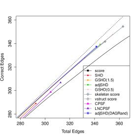
Figure B-7: Learning Curves for Large Graph with $p=504$ nodes, $|\mathbb{E}|=515$ edges, $|\mathbb{VS}|=307$ v-structures and sample size $n=100$, SNR $\in[0.5,1.5]$. Skeleton detection (left): score stops at $(990,430)$; v-structure detection (right): score stops at $(1151,123)$. Dotted line indicates the diagonal line where $\#$ of total $=\#$ of correct.

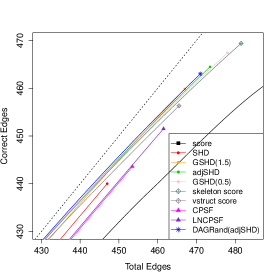
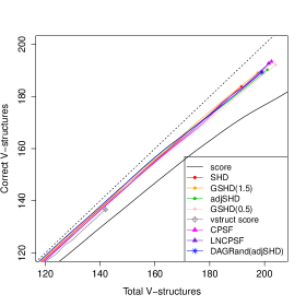
Figure B-8: Learning Curves for Large Graph with $p=504$ nodes, $|\mathbb{E}|=515$ edges, $|\mathbb{VS}|=307$ v-structures and sample size $n=250$, SNR $\in[0.5,1.5]$. Skeleton detection (left): score stops at $(971,494)$; v-structure detection (right): score stops at $(992,212)$. Dotted line indicates the diagonal line where $\#$ of total $=\#$ of correct.

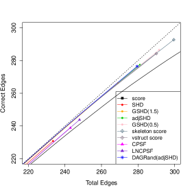
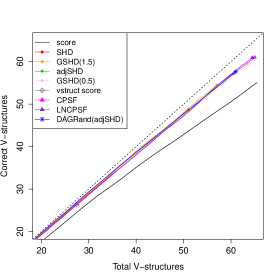
Figure B-9: Learning curves for Large Graph with $p=504,|\mathbb{E}|=515,n=100$, SNR $\in[0.2,0.5]$, skeleton edge curves (left), v-structure curves (right), score stops at $(991.51,371.45)$ on skeleton edge curve and $(1232.6,94.71)$ on v-structure curve.

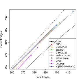
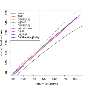
Figure B-10: Learning curves for Large Graph with $p=504,|\mathbb{E}|=515,n=250$, SNR $\in[0.2,0.5]$, skeleton edge curves (left), v-structure curves (right), score stops at $(978.49,451.3)$ on skeleton edge curve and $(1036.51,165.86)$ on v-structure curve.

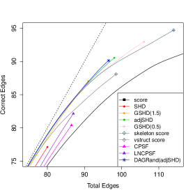
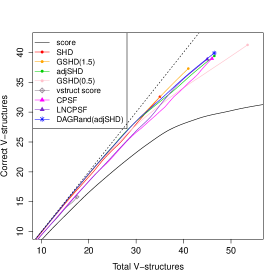
Figure B-11: Learning curves for Sparse Graph with $p=102,|\mathbb{E}|=109,n=102$, SNR $\in[0.5,1.5]$, skeleton edge curves (left), v-structure curves (right), score stops at $(336.79,99.77)$ on skeleton edge curve and $(672.46,36.07)$ on v-structure curve.

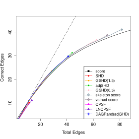
Figure B-12: Skeleton edge learning curve for Sparse Graph with $p=102,|\mathbb{E}|=109,n=102$, SNR $\in[0.2,0.5]$, score stops at $(307.6,58.08)$.

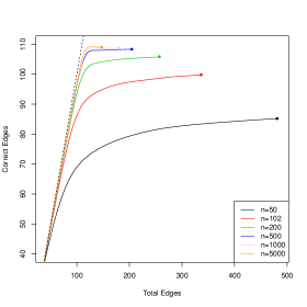
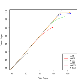
Figure B-13: Skeleton edge learning curves of score (left) and adjSHD (right) under Sparse Graph with $p=102,|\mathbb{E}|=109,\text{SNR}\in[0.5,1.5]$, and $n=50,102,200,500,1000,5000$.

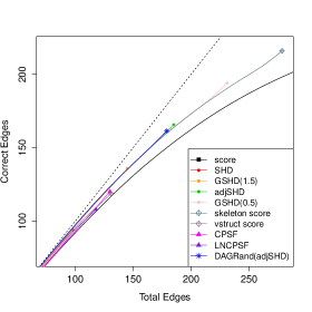
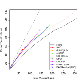
Figure B-14: Learning curves for Dense Graph with $p=104,|\mathbb{E}|=527,n=100$, SNR $\in[0.5,1.5]$, skeleton edge curves (left), v-structure curves (right), score stops at $(524.69,254.70)$ on skeleton edge curve and $(1541.32,206.58)$ on v-structure curve.

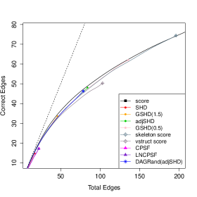
Figure B-15: Learning Curves for Dense Graph with $p=104,|\mathbb{E}|=527,n=100$, SNR $\in[0.2,0.5]$, skeleton edge curves (left), v-structure curves (right), score stops at $(343.9,95.63)$ on skeleton edge curve.

Appendix C-1 Tables

Remark 1

Results are averaged over $100$ independent replicates. Numbers in parenthesis are standard deviations.

Remark 2

• “Total E” – number of skeleton edges in the learned graph; “Correct E” – number of correctly identified skeleton edges in the learned graph;

• “Total V” – number of v-structures in the learned graph; “Correct V” – number of correctly identified v-structures in the learned graph;

• “Total M” – number of edges in the corresponding moral graph of the learned graph; “Correct M” – number of correctly identified moral edges by the learned graph;

• $p$: number of nodes; $|\mathbb{E}|$: number of edges; $n$: sample size; SNR: signal-to-noise-ratio;

• “$100$ bootstrap resamples”: aggregation based on bootstrap resamples; “Independent data”: aggregation based on independent data sets (replicates).

Table C-1: Empty Graph with $p=1000,n=250$.

	Stop/Tuning	Correct E	Total E	Correct V	Total V
score	N.A.	0(0)	1996.1(1.2)	0(0)	3105.3(102)
SHD	N.A.	0(0)	0.1(0.32)	0(0)	0(0)
adjSHD	N.A.	0(0)	6(2.31)	0(0)	0(0)
MMHC	5e-04	0(0)	214.1(10.52)	0(0)	21(3.06)
	0.005	0(0)	1333.1(18.5)	0(0)	814.8(15.87)
	0.05∗	0(0)	4199.6(45.7)	0(0)	9821.1(248.11)
PC-Alg	5e-04	0(0)	203.6(8.6)	0(0)	38.2(5.39)
	0.005∗∗	0(0)	946.5(12.47)	0(0)	560.8(22.44)
	0.01∗∗	0(0)	1433.1(16.43)	0(0)	1231.9(29.4)

^∗ default value set in bnlearn; ^∗∗ values suggested in [17]

Table C-2: Tree Graph with $p=100,|\mathbb{E}|=99$, $n=50$, SNR $\in[0.5,1.5]$.

	Correct E	Total E	Correct V	Total V
score	89.94(2.73)	473.72(8.07)	0	3103.41(543.52)
MST∗	90.44(2.33)	99(0)	0	0
100 bootstrap resamples
SHD(2)	66.08(3.79)	67.58(3.96)	0	2.22(1.44)
GSHD(1.5)	75.03(3.41)	77.27(3.6)	0	5.06(2.25)
adjSHD(1)	78.68(3.26)	82.26(3.47)	0	7.43(2.69)
GSHD(0.5)	81.68(3.02)	87.17(3.21)	0	10.14(3)
Independent data, 100 replicates
SHD(2)	68	68	0	0
GSHD(1.5)	98	98	0	3
adjSHD(1)	99	99	0	4
GSHD(0.5)	99	99	0	4

^∗ minimum spanning tree

Table C-3: Sparse Graph with $p=102,|\mathbb{E}|=109$, v-structure$=77$, Moral Edge$=184$, $n=102$, SNR $\in[0.5,1.5]$.

	Correct E	Total E	Correct V	Total V	correct M	Total M
score	99.77(2.5)	336.79(16.79)	36.07(7.41)	672.46(90.68)	155.4(7.06)	961.38(93.28)
DAGBag, bootstrap
SHD(2)	77.64(4.92)	80.34(5.37)	31.68(6.56)	35.06(7)	110.12(11.11)	115.2(11.62)
GSHD(1.5)	86.62(3.88)	91.4(4.43)	35.11(6.95)	41.25(7.67)	122.69(10.16)	132.35(11.09)
adjSHD(1)	89.87(3.74)	98.43(4.38)	36.78(7.13)	46.94(8.46)	128.17(10.1)	145.02(11.77)
GSHD(0.5)	92.33(3.35)	106.17(4.68)	38.23(7.09)	53.64(8.72)	132.77(9.68)	159.4(12.16)
Independent data, 100 replicates
SHD(2)	99	99	60	60	158	158
GSHD(1.5)	106	106	65	65	170	170
adjSHD(1)	107	107	66	66	172	172
GSHD(0.5)	109	109	72	72	180	180

Table C-4: Sparse Graph with $p=102,|\mathbb{E}|=109$, v-structure$=77$, Moral Edge$=184$, $n=102$, SNR $\in[0.2,0.5]$.

	Correct E	Total E	Correct V	Total V	Correct M	Total M
score	58.08(5.22)	307.6(15.81)	4.83(2.47)	630.08(93.83)	80.37(7.43)	896.58(94.87)
100 bootstrap resamples
SHD(2)	10.76(2.95)	11.98(3.25)	0.17(0.4)	0.84(0.91)	11(3.08)	12.82(3.72)
GSHD(1.5)	23.29(3.61)	28.92(4.06)	0.45(0.63)	3.18(1.74)	24.11(3.81)	32.1(5.02)
adjSHD(1)	30.48(4.17)	44.27(5.03)	0.9(0.82)	8.05(3.05)	32.03(4.47)	52.32(7.26)
GSHD(0.5)	36.12(4.28)	62.62(6.67)	1.42(1.11)	17.44(5.33)	38.65(4.77)	80.04(11.07)
Independent data, 100 replicates
SHD(2)	2	2	0	0	2	2
GSHD(1.5)	23	23	0	1	23	24
adjSHD(1)	34	34	0	1	34	34
GSHD(0.5)	49	49	1	3	50	52

Table C-5: Score comparison on Sparse Graph with $p=102,|\mathbb{E}|=109,n=102,SNR\in[0.5,1.5]$.

	Correct E	Total E	Correct V	Total V	Correct M	Total M
BIC
score	99.77(2.5)	336.79(16.79)	36.07(7.41)	672.46(90.68)	155.4(7.06)	961.38(93.28)
SHD	77.64(4.92)	80.34(5.37)	31.68(6.56)	35.06(7)	110.12(11.11)	115.2(11.62)
adjSHD	89.87(3.74)	98.43(4.38)	36.78(7.13)	46.94(8.46)	128.17(10.1)	145.02(11.77)
like
score	101.13(2.41)	498.59(1.24)	30.98(6.86)	1561.28(117.33)	162.37(6.2)	1802.02(88.53)
SHD	76.46(5.06)	79.46(5.42)	29.08(6.88)	32.52(7.55)	106.6(11.41)	111.84(12.13)
adjSHD	89.76(3.7)	98.84(4.43)	34.13(7.21)	44.39(8.27)	125.9(10.2)	142.92(11.59)
eBIC
score	83.68(4.87)	91.13(5.63)	30.74(7.61)	36.96(7.9)	119.22(12)	127.74(12.25)
SHD	68.33(5.54)	68.97(5.62)	25.65(6.31)	26.45(6.38)	94.37(11.44)	95.31(11.38)
adjSHD	78.87(4.84)	80.07(5.02)	29.63(6.68)	31.17(6.84)	109.03(11.12)	111.09(11.27)
GIC
score	97.2(3.04)	174.39(8.46)	40.59(7.44)	159.61(23.07)	147.56(8.74)	331.05(28.83)
SHD	77.92(4.93)	80.39(5.24)	32.24(7.11)	35.72(7.86)	110.96(11.74)	115.93(12.44)
adjSHD	89.33(3.61)	97.02(4.58)	36.96(6.86)	46.13(8.66)	127.81(9.85)	142.75(12.18)
BGe with $iss=3$
score	101.3(3.2)	218.7(14.27)	54.6(8.45)	286.7(30.68)	157.7(9.18)	497.4(41.59)
SHD	89.2(3.94)	101.2(4.66)	47.6(6.31)	66.5(9.98)	136(9.4)	166.5(13.57)
adjSHD	94.9(3.28)	117.7(4.55)	52.1(6.64)	86.8(12.21)	146.5(8.96)	203(15.66)
BGe with $iss=10$
score	104.1	582.9	52.5(7.95)	2045.8(200.59)	169.1(5.74)	2181.2(149.48)
SHD	91.5(3.47)	115.3(5.01)	49.3(6.48)	86.1(13.7)	140.1(9.19)	199.8(17.66)
adjSHD	98.8(3.29)	166.8(8.38)	55.3(7.23)	163(14.57)	154.4(9.06)	324.7(18.82)

Table C-6: Effect of sample size on Sparse Graph with $p=102,|\mathbb{E}|=109,\text{SNR}\in[0.5,1.5]$.

	Correct E	Total E	Correct V	Total V
n=50
score	85.15(4.36)	482.1(5.71)	21.92(6.12)	3332.9(583.53)
SHD	37.63(4.69)	38.83(4.88)	5.66(2.46)	6.34(2.68)
adjSHD	57.42(5.04)	61.6(5.2)	9.86(3.3)	12.61(3.81)
n=102
score	99.77(2.5)	336.79(16.79)	36.07(7.41)	672.46(90.68)
SHD	77.64(4.92)	80.34(5.37)	31.68(6.56)	35.06(7)
adjSHD	89.87(3.74)	98.43(4.38)	36.78(7.13)	46.94(8.46)
n=200
score	105.78(1.88)	257.3(11.95)	51.49(6.26)	358.46(40.25)
SHD	96.58(3.48)	101.24(4.44)	50.42(6.55)	58.07(7.92)
adjSHD	103.05(2.48)	116.13(4.24)	52.58(6.14)	70.67(9.08)
n=500
score	108.35(0.87)	204.8(9.63)	58.34(5.06)	212.78(23.47)
SHD	104.64(2.12)	111.55(3.56)	61.93(5.4)	74.87(8.13)
adjSHD	107.64(1.13)	124.46(4.69)	61.54(5.03)	84.81(9.24)
n=1000
score	108.71(0.48)	180.85(8.67)	61.74(6.05)	161.24(16.53)
SHD	106.62(1.52)	113.27(3.48)	64.79(4.43)	76.03(6.03)
adjSHD	108.72(0.55)	124.19(4.37)	63.95(4.22)	83.82(7.66)
n=5000
score	108.99(0.1)	147.69(6.79)	65.04(3.89)	106.76(10.47)
SHD	107.68(1.24)	114.09(3.16)	65.18(3.53)	72.82(5.75)
adjSHD	108.97(0.17)	123.19(3.89)	64.02(3.57)	75.26(6.61)

Table C-7: Robustness on Sparse Graph with $p=102,|\mathbb{E}|=109$, $n=102$, SNR $\in[0.5,1.5]$.

	Correct E	Total E	Correct V	Total V	Correct M	Total M
Normal distribution
score	99.77(2.5)	336.79(16.79)	36.07(7.41)	672.46(90.68)	155.4(7.07)	961.38(93.28)
SHD(2)	77.64(4.92)	80.34(5.37)	31.68(6.56)	35.06(7)	110.12(11.11)	115.2(11.62)
GSHD(1.5)	86.62(3.88)	91.4(4.43)	35.11(6.95)	41.25(7.67)	122.69(10.16)	132.35(11.09)
adjSHD(1)	89.87(3.74)	98.43(4.38)	36.78(7.13)	46.94(8.46)	128.17(10.1)	145.02(11.77)
GSHD(0.5)	92.33(3.35)	106.17(4.68)	38.23(7.09)	53.64(8.72)	132.77(9.68)	159.4(12.16)
T-distribution, df=3
score	99.81(2.92)	334.95(17.53)	40.38(6.96)	672.93(94.79)	157.72(7.31)	958.15(98.77)
SHD(2)	79.24(5.71)	82.77(6.09)	35.63(6.76)	40.84(7.59)	115.96(11.8)	123.3(12.91)
GSHD(1.5)	88.13(4.7)	94.46(5.01)	39.23(6.73)	48.05(7.91)	128.54(10.67)	142.02(11.99)
adjSHD(1)	91.29(3.98)	101.98(4.54)	40.81(6.57)	53.83(8.28)	133.72(9.89)	155.21(11.78)
GSHD(0.5)	93.44(3.67)	110.63(5.13)	41.95(6.71)	62.17(8.84)	137.63(9.68)	172.09(12.58)
LN.CPSF	85.15(5.39)	92.57(5.79)	43.03(7.34)	55.39(8.74)	129.7(11.66)	147.31(13.57)
T-distribution, df=5
score	100.43(2.83)	333.51(16.03)	37.85(7.72)	663.69(87.57)	156.74(7.54)	948.72(89.64)
SHD(2)	78.26(4.59)	81.24(4.58)	31.92(6.38)	36.3(6.72)	111.66(10.06)	117.37(10.55)
GSHD(1.5)	87.21(4.09)	92.73(4.65)	35.38(6.47)	42.93(7.45)	124.27(9.31)	135.37(11.03)
adjSHD(1)	90.06(3.84)	99.24(4.74)	36.64(6.41)	47.95(7.91)	128.85(9.13)	146.86(11.51)
GSHD(0.5)	92.79(3.53)	107.81(4.9)	37.77(6.25)	55.4(8.47)	133.36(8.63)	162.76(11.91)
Gamma distribution, shape=1, scale=2
score	99.13(3.04)	330.64(13.65)	39.31(6.5)	655.31(75.97)	155(7.44)	938.3(75.26)
SHD(2)	77.63(4.88)	80.7(5.13)	32.44(5.32)	36.57(6.46)	110.77(9.41)	117.03(10.7)
GSHD(1.5)	86.22(4.38)	91.93(4.75)	35.9(5.29)	43.06(6.66)	123.19(9.17)	134.64(10.52)
adjSHD(1)	89.18(4.12)	99.11(4.52)	37.66(5.5)	49.45(7.51)	128.33(8.9)	148.1(10.8)
GSHD(0.5)	91.71(3.71)	107.84(4.56)	39.05(5.42)	57.37(8.12)	133.01(8.34)	164.63(11.28)

Table C-8: Dense Graph with $p=104,|\mathbb{E}|=527,\text{v-structure}=1675$, Moral $|\mathbb{E}|=1670$, $n=100$, SNR $\in[0.5,1.5]$.

	Correct E	Total E	Correct V	Total V	Correct M	Total M
score	254.7	524.69	206.58	1541.32	822.18	1786.11
	(12.41)	(22.15)	(37.37)	(165.14)	(52.76)	(136.96)
DAGBag
SHD(2)	93.71(9.63)	98.06(9.6)	50.95(14.4)	66.85(16.87)	153.32(23.71)	164.12(25.17)
GSHD(1.5)	134.92(9.95)	145.23(10.08)	78.82(18.11)	122.23(22.94)	233.2(27.1)	264.9(30.98)
adjSHD(1)	164.31(10.02)	185.23(9.91)	104.54(20.03)	189.34(25.81)	303.28(27.63)	368.64(32.71)
GSHD(0.5)	190.93(10.69)	231.02(9.59)	131.03(23.4)	291.17(31.03)	381.01(29.46)	508.7(35.89)
Independent data, 100 replicates
SHD(2)	74	74	47	48	122	122
GSHD(1.5)	119	119	104	106	224	226
adjSHD(1)	153	153	162	170	314	317
GSHD(0.5)	192	192	215	238	410	419

Table C-9: Dense Graph with $p=104,|\mathbb{E}|=527,\text{v-structure}=1675$, Moral edge$=1670$, $n=100$, SNR $\in[0.2,0.5]$.

	Correct E	Total E	Correct V	Total V	Correct M	Total M
score	95.63	343.9	13.16	772.23	384.48	1054.78
	(7.02)	(19.57)	(5.39)	(121.11)	(42.27)	(118.02)
DAGBag
SHD(2)	15.11(4.02)	17.42(4.46)	0.33(0.57)	2.01(1.82)	16.83(4.75)	19.43(5.67)
GSHD(1.5)	33.01(5.09)	46.14(6.31)	1.13(1.2)	10.92(4.5)	41.15(7.16)	57.04(9.93)
adjSHD(1)	47.57(5.58)	84.28(6.68)	2.45(1.9)	36.71(9.14)	70.57(9)	120.83(14.32)
GSHD(0.5)	61.75(6.11)	135.95(8.36)	4.56(2.66)	99.04(16.15)	113.95(11.59)	233.93(22.55)
Independent data, 100 replicates
SHD(2)	2	2	0	0	2	2
GSHD(1.5)	17	17	0	0	17	17
adjSHD(1)	32	32	0	3	32	35
GSHD(0.5)	41	41	0	4	42	45

Table C-10: Large Graph with $p=504,|\mathbb{E}|=515,\text{v-structure}=307$, Moral Edge$=808$, $n=100$, SNR $\in[0.5,1.5]$.

	Correct E	Total E	Correct V	Total V	Correct M	Total M
score	430.3	990.07	123.25	1151.77	585.22	2131.16
	(8.72)	(3.21)	(12.04)	(53.56)	(19.47)	(53.83)
100 bootstrap resamples
SHD(2)	289.25(11.17)	292.92(10.94)	63.47(7.97)	66.3(7.74)	354.66(17.33)	422.07(15.65)
GSHD(1.5)	327.29(9.4)	332.12(9.39)	68.89(8.11)	73.35(7.92)	398.6(16.35)	405.08(16.07)
adjSHD(1)	338.5(8.96)	344.7(8.95)	71.91(8.28)	77.81(8)	413.29(16.07)	422.07(15.65)
GSHD(0.5)	347.12(9.09)	354.98(9.11)	74.57(8.63)	81.78(8.2)	424.82(16.42)	436.28(15.93)
Independent data, 100 replicates
SHD(2)	421	421	178	178	591	591
GSHD(1.5)	463	463	194	195	650	650
adjSHD(1)	473	473	203	207	670	672
GSHD(0.5)	477	478	209	213	681	683

Table C-11: Large Graph with $p=504,|\mathbb{E}|=515,\text{v-structure}=307$, Moral edge$=808$, $n=250$, SNR $\in[0.5,1.5]$ .

	Correct E	Total E	Correct V	Total V	Correct M	Total M
score	494.08	971.41	212.42	992.5	735	1945.78
	(4.94)	(6.2)	(12.07)	(35.9)	(14.73)	(37.82)
100 bootstrap resamples
SHD(2)	440.28(8.57)	447.04(8.64)	182.7(13.07)	191.83(13.13)	624.32(19.95)	633.13(19.89)
GSHD(1.5)	458.99(7.4)	467.37(7.5)	186.54(12.54)	197.97(12.5)	647.71(18.32)	659.35(18.29)
adjSHD(1)	463.29(7.08)	473.57(7.38)	188.72(12.41)	201.37(12.31)	655.34(17.97)	668.87(17.84)
GSHD(0.5)	466.07(7.05)	478.04(7.44)	190.14(12.48)	204.15(12.26)	660.58(17.8)	676(17.68)
Independent data, 100 replicates
SHD(2)	497	497	274	275	758	758
GSHD(1.5)	511	513	275	279	775	776
adjSHD(1)	513	515	275	280	777	779
GSHD(0.5)	507	509	259	263	758	759

Table C-12: Large Graph with $p=504,|\mathbb{E}|=515,\text{v-structure}=307$, Moral Edge$=808$, $n=100$, SNR $\in[0.2,0.5]$.

	Correct E	Total E	Correct V	Total V	Correct M	Total M
score	371.45	991.51	94.71	1232.6	494.96	2214.02
	(12.04)	(2.79)	(13.42)	(64.51)	(22.88)	(64.05)
100 bootstrap resamples
SHD(2)	231.09(11.63)	233.52(11.97)	49(8.48)	51.29(8.57)	281.95(18.6)	284.56(18.86)
GSHD(1.5)	265.86(10.72)	269.23(10.87)	53.94(8.97)	57.1(8.88)	321.77(18.2)	325.99(18.23)
adjSHD(1)	276.54(10.9)	281.1(10.87)	56.55(9.08)	60.6(9.09)	335.34(18.54)	341.31(18.52)
GSHD(0.5)	285.37(10.79)	291.75(10.98)	58.82(9.16)	63.93(9.35)	346.72(18.47)	355.21(18.74)
Independent data, 100 replicates
SHD(2)	271	271	74	74	344	344
GSHD(1.5)	391	391	122	122	511	511
adjSHD(1)	427	427	140	142	565	566
GSHD(0.5)	448	448	160	163	606	607

Table C-13: Large Graph with $p=504,|\mathbb{E}|=515,\text{v-structure}=307$, Moral edge$=808$, $n=250$, SNR $\in[0.2,0.5]$.

	Correct E	Total E	Correct V	Total V	Correct M	Total M
score	451.33	979.49	165.88	1038.99	643.48	2003.73
	(8.74)	(5.03)	(14.15)	(36.97)	(20.52)	(37.33)
100 bootstrap resamples
SHD(2)	365.33(11.02)	370.45(11.17)	137.59(13.9)	144.51(14.48)	504.69(22.42)	511.07(22.91)
GSHD(1.5)	388.42(10.47)	395.17(10.48)	140.9(14.03)	149.57(14.83)	532.02(21.66)	540.71(22.5)
adjSHD(1)	394.57(10.44)	402.67(10.4)	142.64(14.17)	152.46(14.92)	540.38(21.66)	551(22.53)
GSHD(0.5)	399.39(10.5)	409.31(10.45)	144.25(14.45)	155.67(15.59)	547.51(22.36)	560.79(23.35)
Independent data, 100 replicates
SHD(2)	463	463	256	258	707	707
GSHD(1.5)	504	504	268	270	760	760
adjSHD(1)	512	512	268	273	768	770
GSHD(0.5)	512	512	268	273	768	770

Table C-14: Extra-large Graph, $p=1000,|\mathbb{E}|=1068,\text{v-structure}=785$, Moral $|\mathbb{E}|=1823$, $n=100$, SNR $\in[0.5,1.5]$.

	Correct E	Total E	Correct V	Total V	Correct M	Total M
score	881.2	4944.07	317.64	74803.84	1339.19	74325.35
	(13.03)	(9.47)	(22.52)	(4928.25)	(30.62)	(4284.2)
SHD(2)	552.26(18.07)	557.37(18.02)	145.94(12.91)	149.7(13.13)	700.5(29.77)	706.21(29.96)
GSHD(1.5)	625.57(17.04)	632.67(16.96)	162.05(13.4)	167.8(13.72)	790.34(28.99)	799.38(29.41)
adjSHD(1)	654.31(16.56)	663.81(16.55)	171.51(14.08)	179.13(14.32)	828.86(29.2)	841.74(29.43)
GSHD(0.5)	676.94(15.99)	690.17(15.91)	180.23(14.16)	190.86(14.17)	860.94(28.5)	879.78(28.51)

Table C-15: Extra-large Graph, $p=1000,|\mathbb{E}|=1068,\text{v-structure}=785$, Moral $|\mathbb{E}|=1823$, $n=250$,SNR $\in[0.5,1.5]$.

	Correct E	Total E	Correct V	Total V	Correct M	Total M
score	1028.11	4935.95	539.58	17197.54	1648.67	21761.42
	(6.56)	(8.44)	(21.12)	(418.56)	(23.95)	(406.46)
SHD(2)	921.9(12.99)	934.66(13.48)	478.58(24.76)	494.38(25.19)	1398.23(35.21)	1417.66(35.99)
GSHD(1.5)	955.04(12.01)	972.65(13.05)	490.92(24.59)	511.88(25.18)	1445.92(34.14)	1472.74(35.26)
adjSHD(1)	964.23(11.62)	987.12(12.89)	496.74(24.68)	521.67(25.38)	1463.01(34.21)	1496.75(35.55)
GSHD(0.5)	971.4(10.68)	1001.74(12.41)	502.39(24.14)	532.38(25.15)	1478.01(32.67)	1521.87(34.79)

Table C-16: Ultra-large Graph, $p=2639,|\mathbb{E}|=2603,\text{v-structure}=1899$, Moral $|\mathbb{E}|=4481$, $n=250$, SNR $\in[0.5,1.5]$.

	Correct E	Total E	Correct V	Total V	Correct M	Total M
score	2500(11)	9861(11)	1290(40)	26476(3534)	3965(43)	36211(3513)
SHD(2)	2162(24)	2175(24)	1095(42)	1109(43)	3265(63)	3279(64)
GSHD(1.5)	2268(21)	2286(21)	1127(40)	1148(40)	3404(58)	3428(59)
adjSHD(1)	2296(20)	2318(21)	1144(39)	1169(39)	3452(56)	3481(57)
GSHD(0.5)	2317(18)	2344(19)	1158(38)	1188(38)	3489(54)	3526(54)

Table C-17: Bagged estimate of log-likelihood score [9] on Sparse Graph $p=102,|\mathbb{E}|=109,n=102,SNR\in[0.5,1.5]$.

Number of bootstrap resamples	Correct E	Total E
B=10	101	629
B=50	102	511
B=100	102	509
B=500	102	561

References

- [1] Francis R Bach. Bolasso: model consistent lasso estimation through the bootstrap. ICML, 2008.
- [2] C.M. Bishop et al. Pattern recognition and machine learning, volume 4. springer New York, 2006.
- [3] L. Breiman. Bagging predictors. Machine learning, 24(2):123–140, 1996.
- [4] B.M. Broom, K.A. Do, and D. Subramanian. Model averaging strategies for structure learning in bayesian networks with limited data. BMC Bioinformatics, 13(Suppl 13):S10, 2012.
- [5] Jiahua Chen and Zehua Chen. Extended bayesian information criteria for model selection with large model spaces. Biometrika, 95(3):759–771, 2008.
- [6] David Maxwell Chickering. Optimal structure identification with greedy search. The Journal of Machine Learning Research, 3:507–554, 2002.
- [7] D.M. Chickering. Learning equivalence classes of bayesian-network structures. The Journal of Machine Learning Research, 2:445–498, 2002.
- [8] L.M. de Campos and J.F. Huete. Approximating causal orderings for bayesian networks using genetic algorithms and simulated annealing. In Proceedings of the Eight Conference on Information Processing and Management of Uncertainty in Knowledge-Based Systems, pages 333–340, 2000.
- [9] G. Elidan. Bagged structure learning of bayesian networks. 2011.
- [10] G. Elidan, M. Ninio, N. Friedman, and D. Shuurmans. Data perturbation for escaping local maxima in learning. In PROCEEDINGS OF THE NATIONAL CONFERENCE ON ARTIFICIAL INTELLIGENCE, pages 132–139. Menlo Park, CA; Cambridge, MA; London; AAAI Press; MIT Press; 1999, 2002.
- [11] N. Friedman, M. Goldszmidt, and A. Wyner. Data analysis with bayesian networks: A bootstrap approach. In Proceedings of the Fifteenth conference on Uncertainty in artificial intelligence, pages 196–205. Morgan Kaufmann Publishers Inc., 1999.
- [12] N. Friedman, M. Linial, I. Nachman, and D. Pe’er. Using bayesian networks to analyze expression data. Journal of computational biology, 7(3-4):601–620, 2000.
- [13] D. Geiger and D. Heckerman. Learning gaussian networks. In Proceedings of the Tenth international conference on Uncertainty in artificial intelligence, pages 235–243. Morgan Kaufmann Publishers Inc., 1994.
- [14] D. Heckerman. A tutorial on learning with bayesian networks. Innovations in Bayesian Networks, pages 33–82, 2008.
- [15] D. Heckerman, D. Geiger, and D.M. Chickering. Learning bayesian networks: The combination of knowledge and statistical data. Machine learning, 20(3):197–243, 1995.
- [16] S. Imoto, S.Y. Kim, H. Shimodaira, S. Aburatani, K. Tashiro, S. Kuhara, and S. Miyano. Bootstrap analysis of gene networks based on bayesian netowrks and nonparamatric regression. Genome Informatics Series, pages 369–370, 2002.
- [17] M. Kalisch and P. Bühlmann. Estimating high-dimensional directed acyclic graphs with the pc-algorithm. The Journal of Machine Learning Research, 8:613–636, 2007.
- [18] Yongdai Kim, Sunghoon Kwon, and Hosik Choi. Consistent model selection criteria on high dimensions. The Journal of Machine Learning Research, 98888:1037–1057, 2012.
- [19] D. Koller and N. Friedman. Probabilistic graphical models: principles and techniques. MIT press, 2009.
- [20] Joseph B Kruskal. On the shortest spanning subtree of a graph and the traveling salesman problem. Proceedings of the American Mathematical society, 7(1):48–50, 1956.
- [21] S.L. Lauritzen. Graphical models, volume 17. Oxford University Press, USA, 1996.
- [22] S. Li, L. Hsu, J. Peng, and P. Wang. Bootstrap inference for network construction. The Annals of Applied Statistics, 7(1):391–417, 2013.
- [23] Dimitris Margaritis. Learning Bayesian network model structure from data. PhD thesis, University of Pittsburgh, 2003.
- [24] N. Meinshausen and P. Bühlmann. Stability selection. Journal of the Royal Statistical Society: Series B (Statistical Methodology), 72(4):417–473, 2010.
- [25] Elias Chaibub Neto, Mark P Keller, Alan D Attie, and Brian S Yandell. Causal graphical models in systems genetics: a unified framework for joint inference of causal network and genetic architecture for correlated phenotypes. The annals of applied statistics, 4(1):320, 2010.
- [26] Judea Pearl. Causality: models, reasoning and inference, volume 29. Cambridge Univ Press, 2000.
- [27] D. Pe er, A. Regev, G. Elidan, and N. Friedman. Inferring subnetworks from perturbed expression profiles. Bioinformatics, 17(suppl 1):S215–S224, 2001.
- [28] E. Perrier, S. Imoto, and S. Miyano. Finding optimal bayesian network given a super-structure. Journal of Machine Learning Research, 9(2):2251–2286, 2008.
- [29] Robert Clay Prim. Shortest connection networks and some generalizations. Bell system technical journal, 36(6):1389–1401, 1957.
- [30] S.J. Russell, P. Norvig, E. Davis, S.J. Russell, and S.J. Russell. Artificial intelligence: a modern approach. Prentice hall Upper Saddle River, NJ, 2010.
- [31] K. Sachs, O. Perez, D. Pe’er, D.A. Lauffenburger, and G.P. Nolan. Causal protein-signaling networks derived from multiparameter single-cell data. Science Signalling, 308(5721):523, 2005.
- [32] Mark Schmidt, Alexandru Niculescu-Mizil, and Kevin Murphy. Learning graphical model structure using l1-regularization paths. In Proceedings of the National Conference on Artificial Intelligence, volume 22, page 1278. Menlo Park, CA; Cambridge, MA; London; AAAI Press; MIT Press; 1999, 2007.
- [33] M. Scutari. Learning bayesian networks with the bnlearn r package. Journal of Statistical Software, 35(3), 2010.
- [34] P. Spirtes, C. Glymour, and R. Scheines. Causation, prediction, and search, volume 81. MIT press, 2001.
- [35] M. Teyssier and D. Koller. Ordering-based search: A simple and effective algorithm for learning bayesian networks. arXiv preprint arXiv:1207.1429, 2012.
- [36] I. Tsamardinos, L.E. Brown, and C.F. Aliferis. The max-min hill-climbing bayesian network structure learning algorithm. Machine learning, 65(1):31–78, 2006.
- [37] T. Verma and J. Pearl. Equivalence and synthesis of causal models. In Henrion, M., Shachter, R. Kanal, L., and Lemmer, J., editors, Proceeding of the Sixth Conference on Uncertainty in Artificial Intelligence, pages 220–227, 1991.
- [38] S. Wang, B. Nan, S. Rosset, and J. Zhu. Random lasso. The annals of applied statistics, 5(1):468, 2011.
- [39] S. Yaramakala and D. Margaritis. Speculative markov blanket discovery for optimal feature selection. In Data Mining, Fifth IEEE International Conference on, pages 4–pp. IEEE, 2005.