Fast and Flexible ADMM Algorithms for Trend Filtering

Abstract

This paper presents a fast and robust algorithm for trend filtering, a recently developed nonparametric regression tool. It has been shown that, for estimating functions whose derivatives are of bounded variation, trend filtering achieves the minimax optimal error rate, while other popular methods like smoothing splines and kernels do not. Standing in the way of a more widespread practical adoption, however, is a lack of scalable and numerically stable algorithms for fitting trend filtering estimates. This paper presents a highly efficient, specialized ADMM routine for trend filtering. Our algorithm is competitive with the specialized interior point methods that are currently in use, and yet is far more numerically robust. Furthermore, the proposed ADMM implementation is very simple, and importantly, it is flexible enough to extend to many interesting related problems, such as sparse trend filtering and isotonic trend filtering. Software for our method is freely available, in both the C and R languages.

1 Introduction

Trend filtering is a relatively new method for nonparametric regression, proposed independently by Steidl et al. (2006); Kim et al. (2009). Suppose that we are given output points $y=(y_{1},\ldots y_{n})\in\mathbb{R}^{n}$, observed across evenly spaced input points $x=(x_{1},\ldots x_{n})\in\mathbb{R}^{n}$, say, $x_{1}=1,\ldots x_{n}=n$ for simplicity. The trend filtering estimate $\hat{\beta}=(\hat{\beta}_{1},\ldots\hat{\beta}_{n})\in\mathbb{R}^{n}$ of a specified order $k\geq 0$ is defined as

$$\hat{\beta}=\mathop{\mathrm{argmin}}_{\beta\in\mathbb{R}^{n}}\,\frac{1}{2}\|y-\beta\|_{2}^{2}+\lambda\|D^{(k+1)}\beta\|_{1}.$$ (1)

Here $\lambda\geq 0$ is a tuning parameter, and $D^{(k+1)}\in\mathbb{R}^{(n-k)\times n}$ is the discrete difference (or derivative) operator of order $k+1$. We can define these operators recursively as

$$D^{(1)}=\left[\begin{array}[]{rrrrrr}-1&1&0&\ldots&0&0\\ 0&-1&1&\ldots&0&0\\ \vdots&&&&&\\ 0&0&0&\ldots&-1&1\end{array}\right],$$ (2)

and

$$D^{(k+1)}=D^{(1)}D^{(k)}\;\;\;\text{for}\;\,k=1,2,3,\ldots.$$ (3)

(Note that, above, we write $D^{(1)}$ to mean the $(n-k-1)\times(n-k)$ version of the 1st order difference matrix in (2).) When $k=0$, we can see from the definition of $D^{(1)}$ in (2) that the trend filtering problem (1) is the same as the 1-dimensional fused lasso problem (Tibshirani et al., 2005), also called 1-dimensional total variation denoising (Rudin et al., 1992), and hence the 0th order trend filtering estimate $\hat{\beta}$ is piecewise constant across the input points $x_{1},\ldots x_{n}$.

For a general $k$, the $k$th order trend filtering estimate has the structure of a $k$th order piecewise polynomial function, evaluated across the inputs $x_{1},\ldots x_{n}$. The knots in this piecewise polynomial are selected adaptively among $x_{1},\ldots x_{n}$, with a higher value of the tuning parameter $\lambda$ (generally) corresponding to fewer knots. To see examples, the reader can jump ahead to the next subsection, or to future sections. For arbitrary input points $x_{1},\ldots x_{n}$ (i.e., these need not be evenly spaced), the defined difference operators will have different nonzero entries, but their structure and the recursive relationship between them is basically the same; see Section 4.

Broadly speaking, nonparametric regression is a well-studied field with many celebrated tools, and so one may wonder about the merits of trend filtering in particular. For detailed motivation, we refer the reader to Tibshirani (2014), where it is argued that trend filtering essentially balances the strengths of smoothing splines (de Boor, 1978; Wahba, 1990) and locally adaptive regression splines (Mammen & van de Geer, 1997), which are two of the most common tools for piecewise polynomial estimation. In short: smoothing splines are highly computationally efficient but are not minimax optimal (for estimating functions whose derivatives are of bounded variation); locally adaptive regression splines are minimax optimal but are relatively inefficient in terms of computation; trend filtering is both minimax optimal and computationally comparable to smoothing splines. Tibshirani (2014) focuses mainly on the statistical properties trend filtering estimates, and relies on externally derived algorithms for comparisons of computational efficiency.

1.1 Overview of contributions

In this paper, we propose a new algorithm for trend filtering. We do not explicitly address the problem of model selection, i.e., we do not discuss how to choose the tuning parameter $\lambda$ in (1), which is a long-standing statistical issue with any regularized estimation method. Our concern is computational; if a practitioner wants to solve the trend filtering problem (1) at a given value of $\lambda$ (or sequence of values), then we provide a scalable and efficient means of doing so. Of course, a fast algorithm such as the one we provide can still be helpful for model selection, in that it can provide speedups for common techniques like cross-validation.

For 0th order trend filtering, i.e., the 1d fused lasso problem, two direct, linear time algorithms already exist: the first uses a taut string principle (Davies & Kovac, 2001), and the second uses an entirely different dynamic programming approach (Johnson, 2013). Both are extremely (and equally) fast in practice, and for this special $0$th order problem, these two direct algorithms rise above all else in terms of computational efficiency and numerical accuracy. As far as we know (and despite our best attempts), these algorithms cannot be directly extended to the higher order cases $k=1,2,3,\ldots$. However, our proposal indirectly extends these formidable algorithms to the higher order cases with a special implementation of the alternating direction method of multipliers (ADMM). In general, there can be multiple ways to reparametrize an unconstrained optimization problem so that ADMM can be applied; for the trend filtering problem (1), we choose a particular parametrization suggested by the recursive decomposition (3), leveraging the fast, exact algorithms that exist for the $k=0$ case. We find that this choice makes a big difference in terms of the convergence of the resulting ADMM routine, compared to what may be considered the standard ADMM parametrization for (1).

Currently, the specialized primal-dual interior point (PDIP) method of Kim et al. (2009) seems to be the preferred method for computing trend filtering estimates. The iterations of this algorithm are cheap because they reduce to solving banded linear systems (the discrete difference operators are themselves banded). Our specialized ADMM implementation and the PDIP method have distinct strengths. We summarize our main findings below.

• Our specialized ADMM implementation converges more reliably than the PDIP method, over a wide range of problems sizes $n$ and tuning parameter values $\lambda$.

• In particular setups—namely, small problem sizes, and small values of $\lambda$ for moderate and large problem sizes—the PDIP method converges to high accuracy solutions very rapidly. In such situations, our specialized ADMM algorithm does not match the convergence rate of this second-order method.

• However, when plotting the function estimates, our specialized ADMM implementation produces solutions of visually perfectly acceptable accuracy after a small number of iterations. This is true over a broad range of problem sizes $n$ and parameter values $\lambda$, and covers the settings in which its achieved criterion value has not converged at the rate of the PDIP method.

• Furthermore, our specialized ADMM implementation displays a greatly improved convergence rate over what may be thought of as the “standard” ADMM implementation for problem (1). Loosely speaking, standard implementations of ADMM are generally considered to behave like first-order methods (Boyd et al., 2011), whereas our specialized implementation exhibits performance somewhere in between that of a first- and second-order method.

• One iteration of our specialized ADMM implementation has linear complexity in the problem size $n$; this is also true for PDIP. Empirically, an iteration of our ADMM routine runs about 10 times faster than a PDIP iteration.

• Our specialized ADMM implementation is quite simple (considerably simpler than the specialized primal-dual interior point method), and is flexible enough that it can be extended to cover many variants and extensions of the basic trend filtering problem (1), such as sparse trend filtering, mixed trend filtering, and isotonic trend filtering.

• Finally, it is worth remarking that extensions beyond the univariate case are readily available as well, as univariate nonparametric regression tools can be used as building blocks for estimation in broader model classes, e.g., in generalized additive models (Hastie & Tibshirani, 1990).

Readers well-versed in optimization may wonder about alternative iterative (descent) methods for solving the trend filtering problem (1). Two natural candidates that have enjoyed much success in lasso regression problems are proximal gradient and coordinate descent algorithms. Next, we give a motivating case study that illustrates the inferior performance of both of these methods for trend filtering. In short, their performance is heavily affected by poor conditioning of the difference operator $D^{(k+1)}$, and their convergence is many orders of magnitude worse than the specialized primal-dual interior point and ADMM approaches.

1.2 A motivating example

Conditioning is a subtle but ever-present issue faced by iterative (indirect) optimization methods. This issue affects some algorithms more than others; e.g., in a classical optimization context, it is well-understood that the convergence bounds for gradient descent depend on the smallest and largest eigenvalues of the Hessian of the criterion function, while those for Newton’s method do not (Newton’s method being affine invariant). Unfortunately, conditioning is a very real issue when solving the trend filtering problem in (1)—the discrete derivative operators $D^{(k+1)}$, $k=0,1,2,\ldots$ are extremely ill-conditioned, and this only worsens as $k$ increases.

This worry can be easily realized in examples, as we now demonstrate in a simple simulation with a reasonable polynomial order, $k=1$, and a modest problem size, $n=1000$. For solving the trend filtering problem (1), with $\lambda=1000$, we compare proximal gradient descent and accelerated proximal gradient method (performed on both the primal and the dual problems), coordinate descent, a standard ADMM approach, our specialized ADMM approach, and the specialized PDIP method of Kim et al. (2009). Details of the simulation setup and these various algorithms are given in Appendix A.1, but the main message can be seen from Figure 1. Different variants of proximal gradient methods, as well as coordinate descent, and a standard ADMM approach, all perform quite poorly in computing trend filtering estimate, but the second-order PDIP method and our specialized ADMM implementation perform drastically better—these two reach in 20 iterations what the others could not reach in many thousands. Although the latter two techniques perform similarly in this example, we will see later that our specialized ADMM approach generally suffers from far less conditioning and convergence issues than PDIP, especially in regimes of regularization (i.e., ranges of $\lambda$ values) that are most interesting statistically.

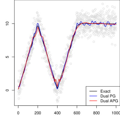
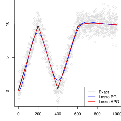
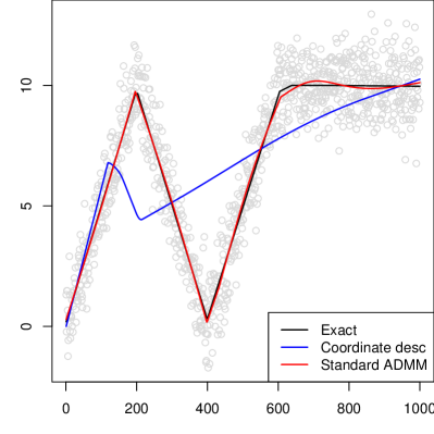
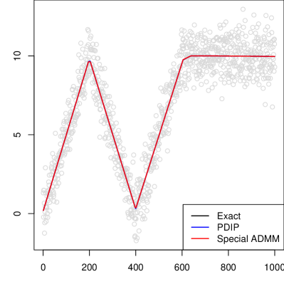
Figure 1: All plots show $n=1000$ simulated observations in gray and the exact trend filtering solution as a black line, computed using the dual path algorithm of Tibshirani & Taylor (2011). The top left panel shows proximal gradient descent and its accelerated version applied to the dual problem, after 10,000 iterations. The top right show proximal gradient and its accelerated version after rewriting trend filtering in lasso form, again after 10,000 iterations. The bottom left shows coordinate descent applied to the lasso form, and a standard ADMM approach applied to the original problem, each using 5000 iterations (where one iteration for coordinate descent is one full cycle of coordinate updates). The bottom right panel shows the specialized PDIP and ADMM algorithms, which only need 20 iterations, and match the exact solution to perfect visual accuracy. Due to the special form of the problem, all algorithms here have $O(n)$ complexity per iteration (except coordinate descent, which has a higher iteration cost).

The rest of this paper is organized as follows. In Section 2, we describe our specialized ADMM implementation for trend filtering. In Section 3, we make extensive comparisons to PDIP. Section 4 covers the case of general input points $x_{1},\ldots x_{n}$. Section 5 considers several extensions of the basic trend filtering model, and the accompanying adaptions of our specialized ADMM algorithm. Section 6 concludes with a short discussion.

2 A specialized ADMM algorithm

We describe a specialized ADMM algorithm for trend filtering. This algorithm may appear to only slightly differ in its construction from a more standard ADMM algorithm for trend filtering, and both approaches have virtually the same computational complexity, requiring $O(n)$ operations per iteration; however, as we have glimpsed in Figure 1, the difference in convergence between the two is drastic.

The standard ADMM approach (e.g., Boyd et al. (2011)) is based on rewriting problem (1) as

$$\min_{\beta\in\mathbb{R}^{n},\,\alpha\in\mathbb{R}^{n-k-1}}\,\frac{1}{2}\|y-\beta\|_{2}^{2}+\lambda\|\alpha\|_{1}\;\;\mathop{\mathrm{subject\,\,to}}\;\;\alpha=D^{(k+1)}\beta.$$ (4)

The augmented Lagrangian can then be written as

$$L(\beta,\alpha,u)=\frac{1}{2}\|y-\beta\|_{2}^{2}+\lambda\|\alpha\|_{1}+\frac{\rho}{2}\|\alpha-D^{(k+1)}\beta+u\|_{2}^{2}-\frac{\rho}{2}\|u\|_{2}^{2},$$

from which we can derive the standard ADMM updates:

$$\beta \leftarrow\big{(}I+\rho(D^{(k+1)})^{T}D^{(k+1)}\big{)}^{-1}\big{(}y+\rho(D^{(k+1)})^{T}(\alpha+u)\big{)},$$ (5)

$$\alpha \leftarrow S_{\lambda/\rho}(D^{(k+1)}\beta-u),$$ (6)

$$u \leftarrow u+\alpha-D^{(k+1)}\beta.$$ (7)

The $\beta$-update is a banded linear system solve, with bandwidth $k+2$, and can be implemented in time $O(n(k+2)^{2})$ (actually, $O(n(k+2)^{2})$ for the first solve, with a banded Cholesky, and $O(n(k+2))$ for each subsequent solve). The $\alpha$-update, where $S_{\lambda/\rho}$ denotes coordinate-wise soft-thresholding at the level $\lambda/\rho$, takes time $O(n-k-1)$. The dual update uses a banded matrix multiplication, taking time $O(n(k+2))$, and therefore one full iteration of standard ADMM updates can be done in linear time (considering $k$ as a constant).

Our specialized ADMM approach instead begins by rewriting (1) as

$$\min_{\beta\in\mathbb{R}^{n},\,\alpha\in\mathbb{R}^{n-k}}\,\frac{1}{2}\|y-\beta\|_{2}^{2}+\lambda\|D^{(1)}\alpha\|_{1}\;\;\mathop{\mathrm{subject\,\,to}}\;\;\alpha=D^{(k)}\beta,$$ (8)

where we have used the recursive property $D^{(k+1)}=D^{(1)}D^{(k)}$. The augmented Lagrangian is now

$$L(\beta,\alpha,u)=\frac{1}{2}\|y-\beta\|_{2}^{2}+\lambda\|D^{(1)}\alpha\|_{1}+\frac{\rho}{2}\|\alpha-D^{(k)}\beta+u\|_{2}^{2}-\frac{\rho}{2}\|u\|_{2}^{2},$$

yielding the specialized ADMM updates:

$$\beta \leftarrow\big{(}I+\rho(D^{(k)})^{T}D^{(k)}\big{)}^{-1}\big{(}y+\rho(D^{(k)})^{T}(\alpha+u)\big{)},$$ (9)

$$\alpha \leftarrow\mathop{\mathrm{argmin}}_{\alpha\in\mathbb{R}^{n-k}}\,\frac{1}{2}\|D^{(k)}\beta-u-\alpha\|_{2}^{2}+\lambda/\rho\|D^{(1)}\alpha\|_{1},$$ (10)

$$u \leftarrow u+\alpha-D^{(k)}\beta.$$ (11)

The $\beta$- and $u$-updates are analogous to those from the standard ADMM, just of a smaller order $k$. But the $\alpha$-update above is not; the $\alpha$-update itself requires solving a constant order trend filtering problem, i.e., a 1d fused lasso problem. Therefore, the specialized approach would not be efficient if it were not for the extremely fast, direct solvers that exist for the 1d fused lasso. Two exact, linear time 1d fused lasso solvers were given by Davies & Kovac (2001), Johnson (2013). The former is based on taut strings, and the latter on dynamic programming. Both algorithms are very creative and are a marvel in their own right; we are more familiar with the dynamic programming approach, and so in our specialized ADMM algorithm, we utilize (a custom-made, highly-optimized implementation of) this dynamic programming routine for the $\alpha$-update, hence writing

$$\alpha\leftarrow\mathrm{DP}_{\lambda/\rho}(D^{(k)}\beta-u).$$ (12)

This uses $O(n-k)$ operations, and thus a full round of specialized ADMM updates runs in linear time, the same as the standard ADMM ones (the two approaches are also empirically very similar in terms of computational time; see Figure 4). As mentioned in the introduction, neither the taut string nor dynamic programming approach can be directly extended beyond the $k=0$ case, to the best of our knowledge, for solving higher order trend filtering problems; however, they can be wrapped up in the special ADMM algorithm described above, and in this manner, they lend their efficiency to the computation of higher order estimates.

2.1 Superiority of specialized over standard ADMM

We now provide further experimental evidence that our specialized ADMM implementation significantly outperforms the naive standard ADMM. We simulated noisy data from three different underlying signals: constant, sinusoidal, and Doppler wave signals (representing three broad classes of functions: trivial smoothness, homogeneous smoothness, and inhomogeneous smoothness). We examined 9 different problem sizes, spaced roughly logarithmically from $n=500$ to $n=500,000$, and considered computation of the trend filtering solution in (1) for the orders $k=1,2,3$. We also considered 20 values of $\lambda$, spaced logarithmically between $\lambda_{\max}$ and $10^{-5}\lambda_{\max}$, where

$$\lambda_{\max}=\big{\|}\big{(}(D^{(k+1)}(D^{(k+1)})^{T}\big{)}^{-1}(D^{(k+1)})^{T}y\big{\|}_{\infty},$$

the smallest value of $\lambda$ at which the penalty term $\|D^{(k+1)}\hat{\beta}\|_{1}$ is zero at the solution (and hence the solution is exactly a $k$th order polynomial). In each problem instance—indexed by the choice of underlying function, problem size, polynomial order $k$, and tuning parameter value $\lambda$—we ran a large number of iterations of the ADMM algorithms, and recorded the achieved criterion values across iterations.

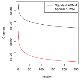
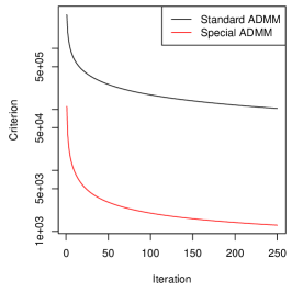
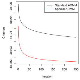
Figure 2: All plots show values of the trend filtering criterion versus iteration number in the two ADMM implementations. The underlying signal here was the Doppler wave, with $n=10,000$, and $k=2$. The left plot shows a large value of $\lambda$ (near $\lambda_{\max}$), the middle a medium value (halfway in between $\lambda_{\max}$ and $10^{-5}\lambda_{\max}$, on a log scale), and the right a small value (equal to $10^{-5}\lambda_{\max}$). The specialized ADMM approach easily outperforms the standard one in all cases.

The results from one particular instance, in which the underlying signal was the Doppler wave, $n=10,000$, and $k=2$, are shown in Figure 2; this instance was chosen arbitrarily, and we have found the same qualitative behavior to persist throughout the entire simulation suite. We can see clearly that in each regime of regularization, the specialized routine dominates the standard one in terms of convergence to optimum. Again, we reiterate that qualitatively the same conclusion holds across all simulation parameters, and the gap between the specialized and standard approaches generally widens as the polynomial order $k$ increases.

2.2 Some intuition for specialized versus standard ADMM

One may wonder why the two algorithms, standard and specialized ADMM, differ so significantly in terms of their performance. Here we provide some intuition with regard to this question. A first, very rough interpretation: the specialized algorithm utilizes a dynamic programming subroutine (12) in place of soft-thresholding (6), therefore solving a more “difficult” subproblem in the same amount of time (linear in the input size), and likely making more progress towards minimizing the overall criterion. In other words, this reasoning follows the underlying intuitive principle that for a given optimization task, an ADMM parametrization with “harder” subproblems will enjoy faster convergence.

While the above explanation was fairly vague, a second, more concrete explanation comes from viewing the two ADMM routines in “basis” form, i.e., from essentially inverting $D^{(k+1)}$ to yield an equivalent lasso form of trend filtering, as explained in (21) of Appendix A.1, where $H^{(k)}$ is a basis matrix. From this equivalent perspective, the standard ADMM algorithm reparametrizes (21) as in

$$\min_{\theta\in\mathbb{R}^{n},\,w\in\mathbb{R}^{n}}\,\frac{1}{2}\|y-H^{(k)}w\|_{2}^{2}+\lambda\cdot k!\sum_{j=k+2}^{n}|\theta_{j}|\;\;\mathop{\mathrm{subject\,\,to}}\;\;w=\theta,$$ (13)

and the specialized ADMM algorithm reparametrizes (21) as in

$$\min_{\theta\in\mathbb{R}^{n},\,w\in\mathbb{R}^{n}}\,\frac{1}{2}\|y-H^{(k-1)}w\|_{2}^{2}+\lambda\cdot k!\sum_{j=k+2}^{n}|\theta_{j}|\;\;\mathop{\mathrm{subject\,\,to}}\;\;w=L\theta,$$ (14)

where we have used the recursion $H^{(k)}=H^{(k-1)}L$ (Wang et al., 2014), analogous (equivalent) to $D^{(k+1)}=D^{(1)}D^{(k)}$. The matrix $L\in\mathbb{R}^{n\times n}$ is block diagonal with the first $k\times k$ block being the identity, and the last $(n-k)\times(n-k)$ block being the lower triangular matrix of 1s. What is so different between applying ADMM to (14) instead of (13)? Loosely speaking, if we ignore the role of the dual variable, the ADMM steps can be thought of as performing alternating minimization over $\theta$ and $w$. The joint criterion being minimized, i.e., the augmented Lagrangian (again hiding the dual variable) is of the form

$$\frac{1}{2}\left\|z-\left[\begin{array}[]{cc}H^{(k)}&0\\ \sqrt{\rho}I&-\sqrt{\rho}I\end{array}\right]\left[\begin{array}[]{cc}\theta\\ w\end{array}\right]\right\|_{2}^{2}+\lambda\cdot k!\sum_{j=k+2}^{n}|\theta_{j}|$$ (15)

for the standard parametrization (13), and

$$\frac{1}{2}\left\|z-\left[\begin{array}[]{cc}H^{(k-1)}&0\\ \sqrt{\rho}I&-\sqrt{\rho}L\end{array}\right]\left[\begin{array}[]{cc}\theta\\ w\end{array}\right]\right\|_{2}^{2}+\lambda\cdot k!\sum_{j=k+2}^{n}|\theta_{j}|$$ (16)

for the special parametrization (14). The key difference between (15) and (16) is that the left and right blocks of the regression matrix in (15) are highly (negatively) correlated (the bottom left and right blocks are each scalar multiples of the identity), but the blocks of the regression matrix in (16) are not (the bottom blocks are the identity and the lower triangular matrix of 1s). Hence, in the context of an alternating minimization scheme, an update step in (16) should make more progress than an update step in (15), because the descent directions for $\theta$ and $w$ are not as adversely aligned (think of coordinatewise minimization over a function whose contours are tilted ellipses, and over one whose contours are spherical). Using the equivalence between the basis form and the original (difference-penalized) form of trend filtering, therefore, we may view the special ADMM updates (9)–(11) as decorrelated versions of the original ADMM updates (5)–(7). This allows each update step to make greater progress in descending on the overall criterion.

2.3 Superiority of warm over cold starts

In the above numerical comparison between special and standard ADMM, we ran both methods with cold starts, meaning that the problems over the sequence of $\lambda$ values were solved independently, without sharing information. Warm starting refers to a strategy in which we solve the problem for the largest value of $\lambda$ first, use this solution to initialize the algorithm at the second largest value of $\lambda$, etc. With warm starts, the relative performance of the two ADMM approaches does not change. However, the performance of both algorithms does improve in an absolute sense, illustrated for the specialized ADMM algorithm in Figure 3.

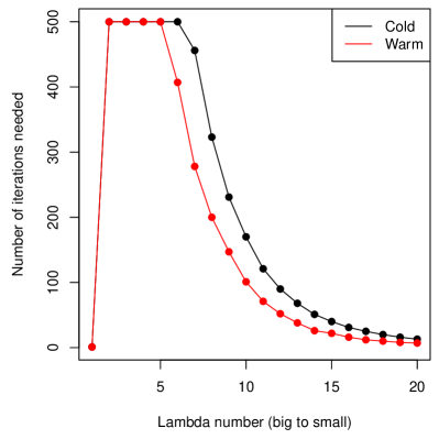
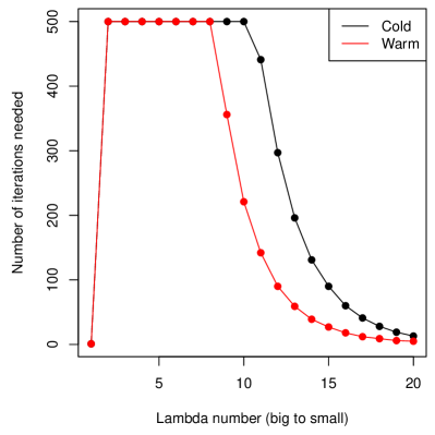
Figure 3: The x-axis in both panels represents 20 values of $\lambda$, log-spaced between $\lambda_{\max}$ and $10^{-5}\lambda_{\max}$, and the y-axis the number of iterations needed by specialized ADMM to reach a prespecified level of accuracy, for $n=10,000$ noisy points from the Doppler curve for $k=2$ (left) and $k=3$ (right). Warm starts (red) have an advantage over cold starts (black), especially in the statistically reasonable (middle) range for $\lambda$.

This example is again representative of the experiments across the full simulation suite. Therefore, from this point forward, we use warm starts for all experiments.

2.4 Choice of the augmented Lagrangian parameter $\rho$

A point worth discussing is the choice of augmented Lagrangian parameter $\rho$ used in the above experiments. Recall that $\rho$ is not a statistical parameter associated with the trend filtering problem (1); it is rather an optimization parameter introduced during the formation of the agumented Lagrangian in ADMM. It is known that under very general conditions, the ADMM algorithm converges to optimum for any fixed value of $\rho$ (Boyd et al., 2011); however, in practice, the rate of convergence of the algorithm, as well as its numerical stability, can both depend strongly on the choice of $\rho$.

We found the choice of setting $\rho=\lambda$ to be numerically stable across all setups. Note that in the ADMM updates (5)–(7) or (9)–(11), the only appearance of $\lambda$ is in the $\alpha$-update, where we apply $S_{\lambda/\rho}$ or $\mathrm{DP}_{\lambda/\rho}$, soft-thresholding or dynamic programming (to solve the 1d fused lasso problem) at the level $\lambda/\rho$. Choosing $\rho$ to be proportional to $\lambda$ controls the amount of change enacted by these subroutines (intuitively making it neither too large nor too small at each step). We also tried adaptively varying $\rho$, a heuristic suggested by Boyd et al. (2011), but found this strategy to be less stable overall; it did not yield consistent benefits for either algorithm.

Recall that this paper is not concerned with the model selection problem of how to choose $\lambda$, but just with the optimization problem of how to solve (1) when given $\lambda$. All results in the rest of this paper reflect the default choice $\rho=\lambda$, unless stated otherwise.

3 Comparison of specialized ADMM and PDIP

Here we compare our specialized ADMM algorithm and the PDIP algorithm of (Kim et al., 2009). We used the C++/LAPACK implementation of the PDIP method (written for the case $k=1$) that is provided freely by these authors, and generalized it to work for an arbitrary order $k\geq 1$. To put the methods on equal footing, we also wrote our own efficient C implementation of the specialized ADMM algorithm. This code has been interfaced to R via the trendfilter function in the R package glmgen, available at https://github.com/statsmaths/glmgen.

A note on the PDIP implementation: this algorithm is actually applied to the dual of (1), as given in (20) in Appendix A.1, and its iterations solve linear systems in the banded matrix $D$ in $O(n)$ time. The number of constraints, and hence the number of log barrier terms, is $2(n-k-1)$. We used 10 for the log barrier update factor (i.e., at each iteration, the weight of log barrier term is scaled by $1/10$). We used backtracking line search to choose the step size in each iteration, with parameters 0.01 and 0.5 (the former being the fraction of improvement over the gradient required to exit, and the latter the step size shrinkage factor). These specific parameter values are the defaults suggested by Boyd & Vandenberghe (2004) for interior point methods, and are very close to the defaults in the original PDIP linear trend filtering code from Kim et al. (2009). In the settings in which PDIP struggled (to be seen in what follows), we tried varying these parameter values, but no single choice led to consistently improved performance.

3.1 Comparison of cost per iteration

Per iteration, both ADMM and PDIP take $O(n)$ time, as explained earlier. Figure 4 reveals that the constant hidden in the $O(\cdot)$ notation is about 10 times larger for PDIP than ADMM. Though the comparisons that follow are based on achieved criterion value versus iteration, it may be kept in mind that convergence plots for the criterion values versus time would be stretched by a factor of 10 for PDIP.

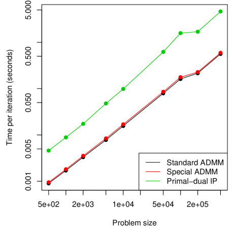
Figure 4: A log-log plot of time per iteration of ADMM and PDIP routines against problem size $n$ (20 values from 500 up to 500,000). The times per iteration of the algorithms were averaged over 3 choices of underlying function (constant, sinusoidal, and Doppler), 3 orders of trends ($k=1,2,3$), 20 values of $\lambda$ (log-spaced between $\lambda_{\max}$ and $10^{-5}\lambda_{\max}$), and 10 repetitions for each combination (except the two largest problem sizes, for which we performed 3 repetitions). This validates the theoretical $O(n)$ iteration complexities of the algorithms, and the larger offset (on the log-log scale) for PDIP versus ADMM implies a larger constant in the linear scaling: an ADMM iteration is about 10 times faster than a PDIP iteration.

3.2 Comparison for $k=1$ (piecewise linear fitting)

In general, for $k=1$ (piecewise linear fitting), both the specialized ADMM and PDIP algorithms perform similarly, as displayed in Figure 5. The PDIP algorithm displays a relative advantage as $\lambda$ becomes small, but the convergence of ADMM is still strong in absolute terms. Also, it is important to note that these small values of $\lambda$ correspond to solutions that overfit the underlying trend in the problem context, and hence PDIP outperforms ADMM in a statistically uninteresting regime of regularization.

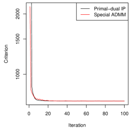
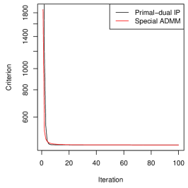
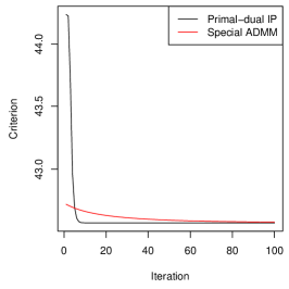
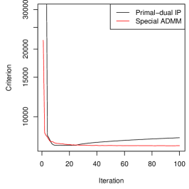
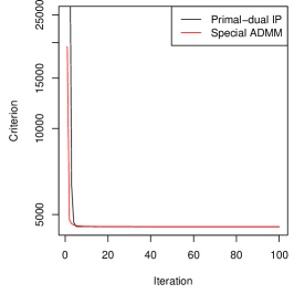
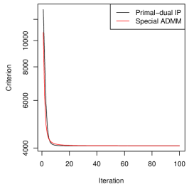
(a) Convergence plots for $k=1$: achieved criterion values across iterations of ADMM and PDIP. The first row concerns $n=10,000$ points, and the second row $n=100,000$ points, both generated around a sinusoidal curve. The columns (from left to right) display high to low values of $\lambda$: near $\lambda_{\max}$, halfway in between (on a log scale) $\lambda_{\max}$ and $10^{-5}\lambda_{\max}$, and equal to $10^{-5}\lambda_{\max}$, respectively. Both algorithms exhibit good convergence.

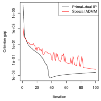
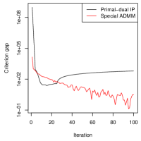
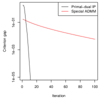
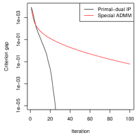
(b) Convergence gaps for $k=1$: achieved criterion value minus the optimum value across iterations of ADMM and PDIP. Here the optimum value was defined as smallest achieved criterion value over 5000 iterations of either algorithm. The first two plots are for $\lambda$ near $\lambda_{\max}$, with $n=10,000$ and $n=100,000$ points, respectively. In this high regularization regime, ADMM fares better for large $n$. The last two plots are for $\lambda=10^{-5}\lambda_{\max}$, with $n=10,000$ and $n=100,000$, respectively. Now in this low regularization regime, PDIP converges at what appears to be a second-order rate, and ADMM does not. However, these small values of $\lambda$ are not statistically interesting in the context of the example, as they yield grossly overfit trend estimates of the underlying sinusoidal curve.

Figure 5: Convergence plots and gaps ($k=1$), for specialized ADMM and PDIP.

3.3 Comparison for $k=2$ (piecewise quadratic fitting)

For $k=2$ (piecewise quadratic fitting), the PDIP routine struggles for moderate to large values of $\lambda$, increasingly so as the problem size grows, as shown in Figure 6. These convergence issues remain as we vary its internal optimization parameters (i.e., its log barrier update parameter, and backtracking parameters). Meanwhile, our specialized ADMM approach is much more stable, exhibiting strong convergence behavior across all $\lambda$ values, even for large problem sizes in the hundreds of thousands.

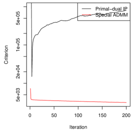
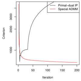
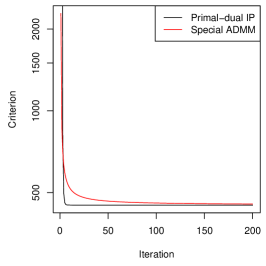
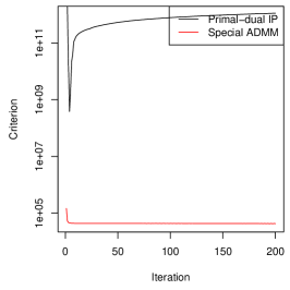
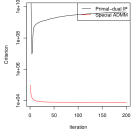
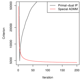
(a) Convergence plots for $k=2$: achieved criterion values across iterations of ADMM and PDIP, with the same layout as in Figure 5(a). The specialized ADMM routine has fast convergence in all cases. For all but the smallest $\lambda$ values, PDIP does not come close to convergence. These values of $\lambda$ are so small that the corresponding trend filtering solutions are not statistically desirable in the first place; see below.

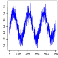
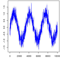
(b) Visualization of trend filtering estimates for the experiments in Figures 5, 6. The estimates were trained on $n=10,000$ points from an underlying sinusoidal curve (but the above plots have been downsampled to 1000 points for visibility). The two left panels show the fits for $k=1,2$, respectively, in the high regularization regime, where $\lambda$ is near $\lambda_{\max}$. The specialized ADMM approach outperforms PDIP (and shown are the ADMM fits). The two right panels show the fits for $k=1,2$, respectively, in the low regularization regime, with $\lambda=10^{-5}\lambda_{\max}$. PDIP converges faster than ADMM (and shown are the PDIP fits), but this is not a statistically reasonable regime for trend estimation.

Figure 6: Convergence plots and estimated fits ($k=2$) for special ADMM and PDIP.

The convergence issues encountered by PDIP here, when $k=2$, are only amplified when $k=3$, as the issues begin to show at much smaller problem sizes; still, the specialized ADMM steadily converges, and is a clear winner in terms of robustness. Analysis of this case is deferred until Appendix A.2 for brevity.

3.4 Some intuition on specialized ADMM versus PDIP

We now discuss some intuition for the observed differences between the specialized ADMM and PDIP. This experiments in this section showed that PDIP will often diverge for large problem sizes and moderate values of the trend order ($k=2,3$), regardless of the choices of the log barrier and backtracking line search parameters. That such behavior presents itself for large $n$ and $k$ suggests that PDIP is affected by poor conditioning of the difference operator $D^{(k+1)}$ in these cases. Since PDIP is affine invariant, in theory it should not be affected by issues of conditioning at all. But when $D^{(k+1)}$ is poorly conditioned, it is difficult to solve the linear systems in $D^{(k+1)}$ that lie at the core of a PDIP iteration, and this leads PDIP to take a noisy update step (like taking a majorization step using a perturbed version of the Hessian). If the computed update directions are noisy enough, then PDIP can surely diverge.

Why does specialized ADMM not suffer the same fate, since it too solves linear systems in each iteration (albeit in $D^{(k)}$ instead of $D^{(k+1)}$)? There is an important difference in the form of these linear systems. Disregarding the order of the difference operator and denoting it simply by $D$, a PDIP iteration solves linear systems (in $x$) of the form

$$(DD^{T}+J)x=b$$ (17)

where $J$ is a diagonal matrix, and an ADMM iteration solves systems of the form

$$(\rho D^{T}D+I)x=b$$ (18)

The identity matrix $I$ provides an important eigenvalue “buffer” for the linear system in (18): the eigenvalues of $\rho D^{T}D+I$ are all bounded away from zero (by 1), which helps make up for the poor conditioning inherent to $D$. Meanwhile, the diagonal elements of $J$ in (17) can be driven to zero across iterations of the PDIP method; in fact, at optimality, complementary slackness implies that $J_{ii}$ is zero whenever the $i$th dual variable lies strictly inside the interval $[-\lambda,\lambda]$. Thus, the matrix $J$ does not always provide the needed buffer for the linear system in (17), so $DD^{T}+J$ can remain poorly conditioned, causing numerical instability issues when solving (17) in PDIP iterations. In particular, when $\lambda$ is large, many dual coordinates will lie strictly inside $[-\lambda,\lambda]$ at optimality, which means that many diagonal elements of $J$ will be pushed towards zero over PDIP iterations. This explains why PDIP experiences particular difficulty in the large $\lambda$ regime, as seen in our experiments.

4 Arbitrary input points

Up until now, we have assumed that the input locations are implicitly $x_{1}=1,\ldots x_{n}=n$; in this section, we discuss the algorithmic extension of our specialized ADMM algorithm to the case of arbitrary input points $x_{1},\ldots x_{n}$. Such an extension is highly important, because, as a nonparametric regression tool, trend filtering is much more likely to be used in a setting with generic inputs than one in which these are evenly spaced. Fortuitously, there is little that needs to be changed with the trend filtering problem (1) when we move from unit spaced inputs $1,\ldots n$ to arbitrary ones $x_{1},\ldots x_{n}$; the only difference is that the operator $D^{(k+1)}$ is replaced by $D^{(x,k+1)}$, which is adjusted for the uneven spacings present in $x_{1},\ldots x_{n}$. These adjusted difference operators are still banded with the same structure, and are still defined recursively. We begin with $D^{(x,1)}=D^{(1)}$, the usual first difference operator in (2), and then for $k\geq 1$, we define, assuming unique sorted points $x_{1}<\ldots<x_{n}$,

$$D^{(x,k+1)}=D^{(1)}\cdot\mathrm{diag}\left(\frac{k}{x_{k+1}-x_{1}},\ldots\frac{k}{x_{n}-x_{n-k}}\right)\cdot D^{(x,k)},$$

where $\mathrm{diag}(a_{1},\ldots a_{m})$ denotes a diagonal matrix with elements $a_{1},\ldots a_{m}$; see Tibshirani (2014); Wang et al. (2014). Abbreviating this as $D^{(x,k+1)}=D^{(1)}\widetilde{D}^{(x,k)}$, we see that we only need to replace $D^{(k)}$ by $\widetilde{D}^{(x,k)}$ in our special ADMM updates, replacing one $(k+1)$-banded matrix with another.

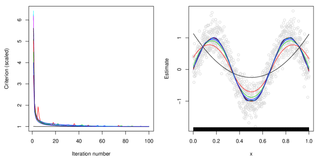
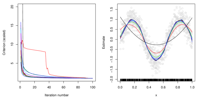
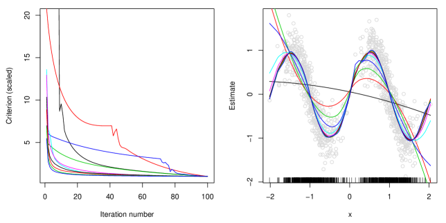
Figure 7: Each row considers a different design for the inputs. Top row: evenly spaced over $[0,1]$; middle row: uniformly at random over $[0,1]$; bottom row: mixture of Gaussians. In each case, we drew $n=1000$ points from a noisy sinusoidal curve at the prescribed inputs. The left panels show the achieved criterion values versus iterations of the specialized ADMM implementation, with $k=2$, the different colored lines show convergence plots at different $\lambda$ values (we used 20 values log-spaced between $\lambda_{\max}$ and $10^{-5}\lambda_{\max}$). The curves are all scaled to end at the same point for visibility. The ADMM algorithm experiences more difficulty as the input spacings become more irregular, due to poorer conditioning of the difference operator. The right panels plot the fitted estimates, with the ticks on the x-axis marking the input locations.

The more uneven the spacings among $x_{1},\ldots x_{n}$, the worse the conditioning of $\tilde{D}^{(x,k)}$, and hence the slower to converge our specialized ADMM algorithm (indeed, the slower to converge any of the alternative algorithms suggested in Section 1.2.) As shown in Figure 7, however, our special ADMM approach is still fairly robust even with considerably irregular design points $x_{1},\ldots x_{n}$.

4.1 Choice of the augmented Lagrangian parameter $\rho$

Aside from the change from $D^{(k)}$ to $\tilde{D}^{(x,k)}$, another key change in the extension of our special ADMM routine to general inputs $x_{1},\ldots x_{n}$ lies in the choice of the augmented Lagrangian parameter $\rho$. Recall that for unit spacings, we argued for the choice $\rho=\lambda$. For arbitrary inputs $x_{1}<\ldots<x_{n}$, we advocate the use of

$$\rho=\lambda\left(\frac{x_{n}-x_{1}}{n}\right)^{k}.$$ (19)

Note that this (essentially) reduces to $\rho=\lambda$ when $x_{1}=1,\ldots x_{n}=n$. To motivate the above choice of $\rho$, consider running two parallel ADMM routines on the same outputs $y_{1},\ldots y_{n}$, but with different inputs: $1,\ldots n$ in one case, and arbitrary but evenly spaced $x_{1},\ldots x_{n}$ in the other. Then, setting $\rho=\lambda$ in the first routine, we choose $\rho$ in the second routine to try to match the first round of ADMM updates as best as possible, and this leads to $\rho$ as in (19). In practice, this input-adjusted choice of $\rho$ makes a important difference in terms of the progress of the algorithm.

5 ADMM algorithms for trend filtering extensions

One of the real strengths of the ADMM framework for solving (1) is that it can be readily adapted to fit modifications of the basic trend filtering model. Here we very briefly inspect some extensions of trend filtering—some of these extensions were suggested by Tibshirani (2014), some by Kim et al. (2009), and some are novel to this manuscript. Our intention is not to deliver an exhaustive list of such extensions (as many more can be conjured), or to study their statistical properties, but rather to show that the ADMM framework is a flexible stage for such creative modeling tasks.

5.1 Sparse trend filtering

In this sparse variant of trend filtering, we aim to estimate a trend that can be exactly zero in some regions of its domain, and can depart from zero in a smooth (piecewise polynomial) fashion. This may be a useful modeling tool when the observations $y_{1},\ldots y_{n}$ represent a difference of signals across common input locations. We solve, as suggested by Tibshirani (2014),

$$\hat{\beta}=\mathop{\mathrm{argmin}}_{\beta\in\mathbb{R}^{n}}\,\frac{1}{2}\|y-\beta\|_{2}^{2}+\lambda_{1}\|D^{(k+1)}\beta\|_{1}+\lambda_{2}\|\beta\|_{1},$$

where both $\lambda_{1},\lambda_{2}$ are tuning parameters. A short calculation yields the specialized ADMM updates:

$$\beta \leftarrow\big{(}(1+\rho_{2})I+\rho_{1}(D^{(k)})^{T}D^{(k)}\big{)}^{-1}\big{(}y+\rho_{1}(D^{(k)})^{T}(\alpha+u)+\rho_{2}(\gamma+v)\big{)},$$

$$\alpha \leftarrow\mathrm{DP}_{\lambda_{1}/\rho_{1}}(D^{(k)}\beta-u),$$

$$\gamma \leftarrow S_{\lambda_{2}/\rho_{2}}(\beta-v),$$

$$u \leftarrow u+\alpha-D^{(k)}\beta,\;\;\;v\leftarrow v+\gamma-\beta.$$

This is still highly efficient, using $O(n)$ operations per iteration. An example is shown in Figure 8.

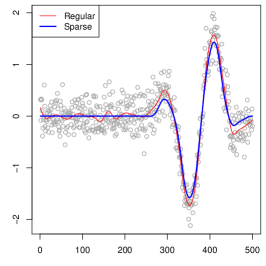
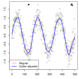
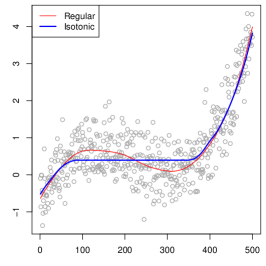
Figure 8: Three examples, of sparse, outlier-corrected, and isotonic trend filtering, from left to right. These extensions of the basic trend filtering model were computed from $n=500$ data points; their fits are drawn in blue, and the original (unmodified) trend filtering solutions are drawn in red, both using the same hand-chosen tuning parameter values. (In the middle panel, the points deemed outliers by the nonzero entries of $\hat{z}$ are colored in black.) These comparisons are not supposed to be statistically fair, but rather, illuminate the qualitative differences imposed by the extra penalties or constraints in the extensions.

5.2 Mixed trend filtering

To estimate a trend with two mixed polynomial orders $k_{1},k_{2}\geq 0$, we solve

$$\hat{\beta}=\mathop{\mathrm{argmin}}_{\beta\in\mathbb{R}^{n}}\,\frac{1}{2}\|y-\beta\|_{2}^{2}+\lambda_{1}\|D^{(k_{1}+1)}\beta\|_{1}+\lambda_{2}\|D^{(k_{2}+1)}\beta\|_{1},$$

as discussed in Tibshirani (2014). The result is that either polynomial trend, of order $k_{1}$ or $k_{2}$, can act as the dominant trend at any location in the domain. More generally, for $r$ mixed polynomial orders, $k_{\ell}\geq 0$, $\ell=1,\ldots r$, we replace the penalty with $\sum_{\ell=1}^{r}\lambda_{\ell}\|D^{(k_{\ell}+1)}\beta\|_{1}$. The specialized ADMM routine naturally extends to this multi-penalty problem:

$$\beta \leftarrow\Big{(}I+\sum_{\ell=1}^{r}\rho_{\ell}(D^{(k_{\ell})})^{T}D^{(k_{\ell})}\Big{)}^{-1}\Big{(}y+\sum_{\ell=1}^{r}\rho_{\ell}(D^{(k_{\ell})})^{T}(\alpha_{\ell}+u_{\ell})\Big{)},$$

$$\alpha_{\ell} \leftarrow\mathrm{DP}_{\lambda_{\ell}/\rho_{\ell}}(D^{(k_{\ell})}\beta-u_{\ell}),\;\;\;\ell=1,\ldots r,$$

$$u_{\ell} \leftarrow u_{\ell}+\alpha_{\ell}-D^{(k_{\ell})}\beta,\;\;\;\ell=1,\ldots r.$$

Each iteration here uses $O(nr)$ operations (recall $r$ is the number of mixed trends).

5.3 Trend filtering with outlier detection

To simultaneously estimate a trend and detect outliers, we solve

$$(\hat{\beta},\hat{z})=\mathop{\mathrm{argmin}}_{\beta,z\in\mathbb{R}^{n}}\,\frac{1}{2}\|y-\beta-z\|_{2}^{2}+\lambda_{1}\|D^{(k+1)}\beta\|_{1}+\lambda_{2}\|z\|_{1},$$

as in Kim et al. (2009), She & Owen (2011), where the nonzero components of $\hat{z}$ correspond to adaptively detected outliers. A short derivation leads to the updates:

$$\begin{pmatrix}\beta\\ z\end{pmatrix} \leftarrow\left(\begin{array}[]{cc}I+\rho_{1}(D^{(k)})^{T}D^{(k)}&I\\ I&(1+\rho_{2})I\end{array}\right)^{-1}\left(\begin{array}[]{c}y+\rho_{1}(D^{(k)})^{T}(\alpha+u)\\ y+\rho_{2}(\gamma+v)\end{array}\right),$$

$$\alpha \leftarrow\mathrm{DP}_{\lambda_{1}/\rho_{1}}(D^{(k)}\beta-u),$$

$$\gamma \leftarrow S_{\lambda_{2}/\rho_{2}}(z-v),$$

$$u \leftarrow u+\alpha-D^{(k)}\beta,\;\;\;v\leftarrow v+\gamma-z.$$

Again, this routine uses $O(n)$ operations per iteration. See Figure 8 for an example.

5.4 Isotonic trend filtering

A monotonicity constraint in the estimated trend is straightforward to encode:

$$\hat{\beta}=\mathop{\mathrm{argmin}}_{\beta\in\mathbb{R}^{n}}\,\frac{1}{2}\|y-\beta\|_{2}^{2}+\lambda\|D^{(k+1)}\beta\|_{1}\;\;\mathop{\mathrm{subject\,\,to}}\;\;\beta_{1}\leq\beta_{2}\leq\ldots\leq\beta_{n},$$

as suggested by Kim et al. (2009). The specialized ADMM updates are easy to derive:

$$\beta \leftarrow\big{(}(1+\rho_{2})I+\rho_{1}(D^{(k)})^{T}D^{(k)}\big{)}^{-1}\big{(}y+\rho_{1}(D^{(k)})^{T}(\alpha+u)+\rho_{2}(\gamma+v)\big{)},$$

$$\alpha \leftarrow\mathrm{DP}_{\lambda/\rho}(D^{(k)}\beta-u),$$

$$\gamma \leftarrow\mathrm{IR}(\beta-v),$$

$$u \leftarrow u+\alpha-D^{(k)}\beta,\;\;\;v\leftarrow v+\gamma-\beta.$$

where $\mathrm{IR}(z)$ denotes an isotonic regression fit on $z$; since this takes $O(n)$ time (e.g., Stout (2008)), a round of updates also takes $O(n)$ time. Figure 8 gives an example.

5.5 Nearly-isotonic trend filtering

Instead of enforcing strict monotonicity in the fitted values, we can penalize the pointwise nonmontonicities with a separate penalty, following Tibshirani et al. (2011):

$$\hat{\beta}=\mathop{\mathrm{argmin}}_{\beta\in\mathbb{R}^{n}}\,\frac{1}{2}\|y-\beta\|_{2}^{2}+\lambda_{1}\|D^{(k+1)}\beta\|_{1}+\lambda_{2}\sum_{i=1}^{n-1}(\beta_{i}-\beta_{i+1})_{+}.$$

This results in a “nearly-isotonic” fit $\hat{\beta}$. Above, we use $x_{+}=\max\{x,0\}$ to denote the positive part of $x$. The specialized ADMM updates are:

$$\beta \leftarrow\big{(}(1+\rho_{2})I+\rho_{1}(D^{(k)})^{T}D^{(k)}\big{)}^{-1}\big{(}y+\rho_{1}(D^{(k)})^{T}(\alpha+u)+\rho_{2}(\gamma+v)\big{)},$$

$$\alpha \leftarrow\mathrm{DP}_{\lambda_{1}/\rho_{1}}(D^{(k)}\beta-u),$$

$$\gamma \leftarrow\mathrm{DP}_{\lambda_{2}/\rho_{2}}^{+}(\beta-v),$$

$$u \leftarrow u+\alpha-D^{(k)}\beta,\;\;\;v\leftarrow v+\gamma-\beta.$$

where $\mathrm{DP}_{t}^{+}(z)$ denotes a nearly-isotonic regression fit to $z$, with penalty parameter $t$. It can be computed in $O(n)$ time by modifying the dynamic programming algorithm of Johnson (2013) for the 1d fused lasso, so one round of updates still takes $O(n)$ time.

6 Conclusion

We proposed a specialized but simple ADMM approach for trend filtering, leveraging the strength of extremely fast, exact solvers for the special case $k=0$ (the 1d fused lasso problem) in order to solve higher order problems with $k\geq 1$. The algorithm is fast and robust over a wide range of problem sizes and regimes of regularization parameters (unlike primal-dual interior point methods, the current state-of-the-art). Our specialized ADMM algorithm converges at a far superior rate to (accelerated) first-order methods, coordinate descent, and (what may be considered as) the standard ADMM approach for trend filtering. Finally, a major strength of our proposed algorithm is that it can be modified to solve many extensions of the basic trend filtering problem. Software for our specialized ADMM algorithm is accessible through the trendfilter function in the R package glmgen, built around a lower level C package, both freely available at https://github.com/statsmaths/glmgen.

Acknowledgements. Taylor Arnold and Veeranjaneyulu Sadhanala contributed tremendously to the development of the new glmgen package. We thank the anonymous Associate Editor and Referees for their very helpful reading of our manuscript. This work was supported by NSF Grant DMS-1309174.

Appendix A Appendix: further details and simulations

A.1 Algorithm details for the motivating example

First, we examine in Figure 9 the condition numbers of the discrete difference operators $D^{(k+1)}\in\mathbb{R}^{(n-k-1)\times n}$, for varying problem sizes $n$, and $k=0,1,2$. Since the plot uses a log-log scale, the straight lines indicate that the condition numbers grow polynomially with $n$ (with a larger exponent for larger $k$). The sheer size of the condition numbers (which can reach $10^{10}$ or larger, even for a moderate problem size of $n=5000$) is worrisome from an optimization point of view; roughly speaking, we would expect the criterion in these cases to be very flat around its optimum.

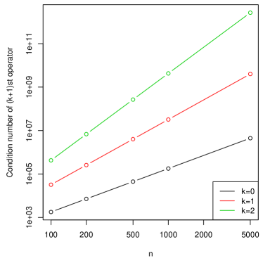
Figure 9: A log-log plot of the condition number of $D^{(k+1)}$ versus the problem size $n$, for $k=0,1,2$, where the condition numbers scale roughly like $n^{k}$.

Figure 1 (in the introduction) provides evidence that such a worry can be realized in practice, even with only a reasonable polynomial order and moderate problem size. For this example, we drew $n=1000$ points from an underlying piecewise linear function, and studied computation of the linear trend filtering estimate, i.e., with $k=1$, when $\lambda=1000$. We chose this tuning parameter value because it represents a statistically reasonable level of regularization in the example. The exact solution of the trend filtering problem at $\lambda=1000$ was computed using the generalized lasso dual path algorithm (Tibshirani & Taylor 2011, Arnold & Tibshirani 2014). The problem size here is small enough that this algorithm, which tracks the solution in (1) as $\lambda$ varies continuously from $\infty$ to 0, can be run effectively; however, for larger problem sizes, computation of the full solution path quickly becomes intractable. Each panel of Figure 1 plots the simulated data points, and the exact solution as a reference point. The results of using various algorithms to solve (1) at $\lambda=1000$ are also shown. Below we give the details of these algorithms.

• Proximal gradient algorithms cannot be used directly to solve the primal problem (1) (note that evaluating the proximal operator is the same as solving the problem itself). However, proximal gradient descent can be applied to the dual of (1). Abbreviating $D=D^{(k+1)}$, the dual problem can be expressed as (e.g., see Tibshirani & Taylor (2011))

  $$\hat{u}=\mathop{\mathrm{argmin}}_{u\in\mathbb{R}^{n-k-1}}\,\|y-D^{T}u\|_{2}^{2}\;\;\mathop{\mathrm{subject\,\,to}}\;\;\|u\|_{\infty}\leq\lambda.$$ (20)

  The primal and dual solutions are related by $\hat{\beta}=y-D^{T}\hat{u}$. We ran proximal gradient and accelerated proximal gradient descent on (20), and computed primal solutions accordingly. Each iteration here is very efficient and requires $O(n)$ operations, as computation of the gradient involves one multiplication by $D$ and one by $D^{T}$, which takes linear time since these matrices are banded, and the proximal operator is simply coordinate-wise truncation (projection onto an $\ell_{\infty}$ ball). The step sizes for each algorithm were hand-selected to be the largest values for which the algorithms still converged; this was intended to give the algorithms the best possible performance. The top left panel of Figure 1 shows the results after 10,000 iterations of proximal gradient its accelerated version on the dual (20). The fitted curves are wiggly and not piecewise linear, even after such an unreasonably large number of iterations, and even with acceleration (though acceleration clearly provides an improvement).

• The trend filtering problem in (1) can alternatively be written in lasso form,

  $$\hat{\theta}=\mathop{\mathrm{argmin}}_{\theta\in\mathbb{R}^{n}}\,\frac{1}{2}\|y-H\theta\|_{2}^{2}+\lambda\cdot k!\sum_{j=k+2}^{n}|\theta_{j}|,$$ (21)

  where $H=H^{(k)}\in\mathbb{R}^{n\times n}$ is $k$th order falling factorial basis matrix, defined over $x_{1},\ldots x_{n}$, which, recall, we assume are $1,\ldots n$. The matrix $H$ is effectively the inverse of $D$ (Tibshirani 2014), and the solutions of (1) and (21) obey $\hat{\beta}=H\hat{\theta}$. The lasso problem (21) provides us with another avenue for proximal gradient descent. Indeed the iterations of proximal gradient descent on (21) are very efficient and can still be done in $O(n)$ time: the gradient computation requires one multiplication by $H$ and $H^{T}$, which can be applied in linear time, despite the fact that these matrices are dense (Wang et al. 2014), and the proximal map is coordinate-wise soft-thresholding. After 10,000 iterations, as we can see from the top right panel of Figure 1, this method still gives an unsatisfactory fit, and the same is true for 10,000 iterations with acceleration (the output here is close, but it is not piecewise linear, having rounded corners).

• The bottom left panel in the figure explores two commonly used non-first-order methods, namely, coordinate descent applied to the lasso formulation (21), and a standard ADMM approach on the original formulation (1). The standard ADMM algorithm is described in Section 2, and has $O(n)$ per iteration complexity. As far as we can tell, coordinate descent requires $O(n^{2})$ operations per iteration (one iteration being a full cycle of coordinate-wise minimizations), because the update rules involve multiplication by individual columns of $H$, and not $H$ in its entirety. The plot shows the results of these two algorithms after 5000 iterations each. After such a large number of iterations, the standard ADMM result is fairly close to the exact solution in some parts of the domain, but overall fails to capture the piecewise linear structure. Coordinate descent, on the other hand, is quite far off (although we note that it does deliver a visually perfect piecewise linear fit after nearly 100,000 iterations).

• The bottom right panel in the figure justifies the perusal of this paper, and should generate excitement in the curious reader. It illustrates that after just 20 iterations, both the PDIP method of Kim et al. (2009), and our special ADMM implementation deliver results that are visually indistinguishable from the exact solution. In fact, after only $5$ iterations, the specialized ADMM fit (not shown) is visually passable. Both algorithms use $O(n)$ operations per iteration: the PDIP algorithm is actually applied to the dual problem (20), and its iterations reduce to solving linear systems in the banded matrix $D$; the special ADMM algorithm in described in Section 2.

A.2 ADMM vs. PDIP for $k=3$ (piecewise cubic fitting)

For the case $k=3$ (piecewise cubic fitting), the behavior of PDIP mirrors that in the $k=2$ case, yet the convergence issues begin to show at problem sizes smaller by an order of magnitude. The specialized ADMM approach is slightly slower to converge, but overall still quite fast and robust. Figure 10 supports this point.

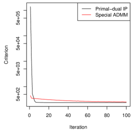
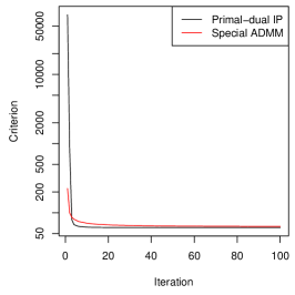
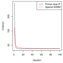
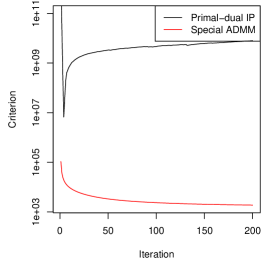
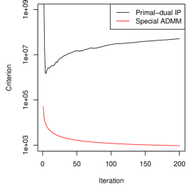
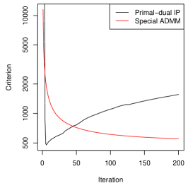
Figure 10: Convergence plots for ($k=3$): achieved criterion values across iterations of ADMM and PDIP, with the same layout as in Figures 5(a) and 6(a), except that the first row uses $n=1000$ points, and the second row $n=10,000$ points. Both algorithms comfortably converge when $n=1000$. However, PDIP encounters serious difficulties when $n=10,000$, reminiscent of its behavior for $k=2$ but when $n=100,000$ (see Figure 6(a)). In all cases, the specialized ADMM algorithm demonstrates a strong and steady convergence behavior.

A.3 Prediction at arbitrary points

Continuing within the nonparametric regression context, an important task to consider is that of function prediction at arbitrary locations in the domain. We discuss how to make such predictions using trend filtering. This topic is not directly relevant to our particular algorithmic proposal, but our R software package that implements this algorithm also features the function prediction task, and hence we describe it here for completeness. The trend filtering estimate, as defined in (1), produces fitted values $\hat{\beta}_{1},\ldots\hat{\beta}_{n}$ at the given input points $x_{1},\ldots x_{n}$. We may think of these fitted values as the evaluations of an underlying fitted function $\hat{f}$, as in $\big{(}\hat{f}(x_{1}),\ldots\hat{f}(x_{n})\big{)}=(\hat{\beta}_{1},\ldots\hat{\beta}_{n}).$ Tibshirani (2014), Wang et al. (2014) argue that the appropriate extension of $\hat{f}$ to the continuous domain is given by

$$\hat{f}(x)=\sum_{j=1}^{k+1}\hat{\phi}_{j}\cdot h_{j}(x)+\sum_{j=1}^{n-k-1}\hat{\theta}_{j}\cdot h_{k+1+j}(x),$$ (22)

where $h_{1},\ldots h_{n}$ are the falling factorial basis functions, defined as

$$h_{j}(x)=\prod_{\ell=1}^{j-1}(x-x_{\ell}),\;\;\;j=1,\ldots k+1,$$

$$h_{k+1+j}(x)=\prod_{\ell=1}^{k}(x-x_{j+\ell})\cdot 1\{x\geq x_{j+k}\},\;\;\;j=1,\ldots n-k-1,$$

and $\hat{\phi}\in\mathbb{R}^{k+1}$, $\hat{\theta}\in\mathbb{R}^{n-k-1}$ are inverse coefficients to $\hat{\beta}$. The first $k+1$ coefficients index the polynomial functions $h_{1},\ldots h_{k+1}$, and defined by $\hat{\phi}_{1}=\hat{\beta}_{1}$, and

$$\hat{\phi}_{j}=\frac{1}{(j-1)!}\cdot\left[\mathrm{diag}\left(\frac{1}{x_{j}-x_{1}},\ldots\frac{1}{x_{n}-x_{n-j+1}}\right)\cdot D^{(x,j-1)}\right]_{1}\cdot\hat{\beta},\;\;\;j=2,\ldots k+1.$$ (23)

Above, we use $A_{1}$ to denote the first row of a matrix $A$. Note that $\hat{\phi}_{1},\ldots\hat{\phi}_{k+1}$ are generally nonzero at the trend filtering solution $\hat{\beta}$. The last $n-k-1$ coefficients index the knot-producing functions $h_{k+2},\ldots h_{n}$, and are defined by

$$\hat{\theta}=D^{(x,k+1)}\hat{\beta}/k!.$$ (24)

Unlike $\hat{\phi}$, it is apparent that many of $\hat{\theta}_{1},\ldots\hat{\theta}_{n-k-1}$ will be zero at the trend filtering solution, more so for large $\lambda$. Given a trend filtering estimate $\hat{\beta}$, we can precompute the coefficients $\hat{\phi},\hat{\theta}$ as in (23). Then, to produce evaluations of the underlying estimated function $\hat{f}$ at arbitrary points $x^{\prime}_{1},\ldots x^{\prime}_{m}$, we calculate the linear combinations of falling factorial basis functions according to (22). From the precomputed coefficients $\hat{\phi},\hat{\theta}$, this requires only $O(mr)$ operations, where $r=\|D^{(x,k+1)}\hat{\beta}\|_{0}$, the number of nonzero $(k+1)$st order differences at the solution (we are taking $k$ to be a constant).

References

- (1)
- Arnold & Tibshirani (2014) Arnold, T. & Tibshirani, R. J. (2014), Efficient implementations of the generalized lasso dual path algorithm. arXiv: 1405.3222.
- Boyd et al. (2011) Boyd, S., Parikh, N., Chu, E., Peleato, B. & Eckstein, J. (2011), ‘Distributed optimization and statistical learning via the alternative direction method of multipliers’, Foundations and Trends in Machine Learning 3(1), 1–122.
- Boyd & Vandenberghe (2004) Boyd, S. & Vandenberghe, L. (2004), Convex Optimization, Cambridge University Press, Cambridge.
- Davies & Kovac (2001) Davies, P. L. & Kovac, A. (2001), ‘Local extremes, runs, strings and multiresolution’, Annals of Statistics 29(1), 1–65.
- de Boor (1978) de Boor, C. (1978), A Practical Guide to Splines, Springer, New York.
- Hastie & Tibshirani (1990) Hastie, T. & Tibshirani, R. (1990), Generalized additive models, Chapman and Hall, London.
- Johnson (2013) Johnson, N. (2013), ‘A dynamic programming algorithm for the fused lasso and -segmentation’, Journal of Computational and Graphical Statistics 22(2), 246–260.
- Kim et al. (2009) Kim, S.-J., Koh, K., Boyd, S. & Gorinevsky, D. (2009), ‘ trend filtering’, SIAM Review 51(2), 339–360.
- Mammen & van de Geer (1997) Mammen, E. & van de Geer, S. (1997), ‘Locally apadtive regression splines’, Annals of Statistics 25(1), 387–413.
- Rudin et al. (1992) Rudin, L. I., Osher, S. & Faterni, E. (1992), ‘Nonlinear total variation based noise removal algorithms’, Physica D: Nonlinear Phenomena 60, 259–268.
- She & Owen (2011) She, Y. & Owen, A. B. (2011), ‘Outlier detection using nonconvex penalized regression’, Journal of the American Statistical Association: Theory and Methods 106(494), 626–639.
- Steidl et al. (2006) Steidl, G., Didas, S. & Neumann, J. (2006), ‘Splines in higher order TV regularization’, International Journal of Computer Vision 70(3), 214–255.
- Stout (2008) Stout, Q. (2008), ‘Unimodal regression via prefix isotonic regression’, Computational Statistics and Data Analysis 53(2), 289–297.
- Tibshirani (2014) Tibshirani, R. J. (2014), ‘Adaptive piecewise polynomial estimation via trend filtering’, Annals of Statistics 42(1), 285–323.
- Tibshirani et al. (2011) Tibshirani, R. J., Hoefling, H. & Tibshirani, R. (2011), ‘Nearly-isotonic regression’, Technometrics 53(1), 54–61.
- Tibshirani & Taylor (2011) Tibshirani, R. J. & Taylor, J. (2011), ‘The solution path of the generalized lasso’, Annals of Statistics 39(3), 1335–1371.
- Tibshirani et al. (2005) Tibshirani, R., Saunders, M., Rosset, S., Zhu, J. & Knight, K. (2005), ‘Sparsity and smoothness via the fused lasso’, Journal of the Royal Statistical Society: Series B 67(1), 91–108.
- Wahba (1990) Wahba, G. (1990), Spline Models for Observational Data, Society for Industrial and Applied Mathematics, Philadelphia.
- Wang et al. (2014) Wang, Y., Smola, A. & Tibshirani, R. J. (2014), ‘The falling factorial basis and its statistical properties’, International Conference on Machine Learning 31.