Training Convolutional Networks
with Noisy Labels
Abstract
The availability of large labeled datasets has allowed Convolutional Network models to achieve impressive recognition results. However, in many settings manual annotation of the data is impractical; instead our data has noisy labels, i.e. there is some freely available label for each image which may or may not be accurate. In this paper, we explore the performance of discriminatively-trained Convnets when trained on such noisy data. We introduce an extra noise layer into the network which adapts the network outputs to match the noisy label distribution. The parameters of this noise layer can be estimated as part of the training process and involve simple modifications to current training infrastructures for deep networks. We demonstrate the approaches on several datasets, including large scale experiments on the ImageNet classification benchmark.
1 Introduction
In recent years, Convolutional Networks (Convnets) (LeCun et al., 1989; Lecun et al., 1998) have shown impressive results on image classification tasks (Krizhevsky et al., 2012; Simonyan & Zisserman, 2014). However, this achievement relies on the availability of large amounts of labeled images, e.g. ImageNet (Deng et al., 2009). Labeling images by hand is a laborious task and impractical for many problems. An alternative approach is to use labels that can be obtained easily, such as user tags from social network sites, or keywords from image search engines. The catch is that these labels are not reliable so they may contain misleading information that will subvert the model during training. But given the abundance of tasks where noisy labels are available, it is important to understand the consequences of training a Convnet on them, and this is one of the contributions of our paper.
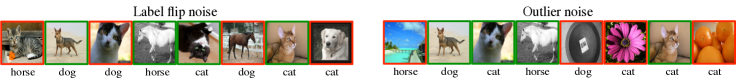
For image classification in real-world settings, two types of label noise dominate: (i) label flips, where an example has erroneously been given the label of another class within the dataset and (ii) outliers, where the image does not belong to any of the classes under consideration, but mistakenly has one of their labels. Fig. 1 shows examples of these two cases. We consider both scenarios and explore them on a variety of noise levels and datasets. Contrary to expectations, a standard Convnet model (from Krizhevsky et al. (2012)) proves to be surprisingly robust to both types of noise. But inevitably, at high noise levels significant performance degradation occurs.
Consequently, we propose a novel modification to a Convnet that enables it to be effectively trained on data with high level of label noise. The modification is simply done by adding a constrained linear “noise” layer on top of the softmax layer which adapts the softmax output to match the noise distribution. We demonstrate that this model can handle both label flip and outlier noise. As it is a linear layer, both it and the rest of the model can be trained end-to-end with conventional back-propagation, thus automatically learning the noise distribution without supervision. The model is also easy to implement with existing Convnet libraries (Krizhevsky, 2012; Jia et al., 2014; Collobert et al., 2011) and can readily scale to ImageNet-sized problems.
2 Related Work
In any classification model, a degradation in performance is inevitable when there is noise in the training data (Nettleton et al., 2010; Pechenizkiy et al., 2006). Especially, noise in labels is more harmful than noise in input features (Zhu & Wu, 2004). Label noise itself is a complex phenomenon. There are several types of noise on labels (Frenay & Verleysen, 2014). Also, noise source can be very different. For example, label noise can be caused by unreliable labeling by cheap and fast framework such as Amazon Mechanical Turk (http://www.mturk.com) (Ipeirotis et al., 2010), or noise can be introduced to labels intentionally to protect people privacy (van den Hout & van der Heijden, 2002).
A simple approach to handle noisy labels is a data preprocessing stage, where labels suspected to be incorrect are removed or corrected (Barandela & Gasca, 2000; Brodley & Friedl, 1999). However, a weakness of this approach is the difficulty of distinguishing informative hard samples from harmful mislabeled ones (Guyon et al., 1996). Instead, in this paper, we focus on models robust to presence of label noise. The effects of label noise are well studied in common classifiers (e.g. SVMs, kNN, logistic regression), and robust variants have been proposed (Frenay & Verleysen, 2014; Bootkrajang & Kab n, 2012). Recently, Natarajan et al. (2013) proposed a generic unbiased estimator for binary classification with noisy labels. They employed a surrogate cost function that can be expressed by a weighted sum of the original cost functions, and gave theoretical bounds on the performance.
Considering the recent success of deep learning (Krizhevsky et al., 2012; Taigman et al., 2014; Sermanet et al., 2014), there is relatively little work on their application to noisy data. In Mnih & Hinton (2012) and Larsen et al. (1998), noise modeling is incorporated to neural network in the same way as our proposed model. However, only binary classification is considered in Mnih & Hinton (2012), and Larsen et al. (1998) assumed symmetric label noise (i.e. noise is independent of the true label). Therefore, there is only a single noise parameter, which can be tuned by cross-validation. In this paper, we consider multi-class classification and assume more realistic asymmetric label noise, which makes it impossible to use cross-validation to adjust noise parameters (for classes, there are parameters). Unsupervised pre-training of deep models has received much attention (Hinton & Salakhutdinov, 2006; Erhan et al., 2010). Particularly relevant to our work is Le (2013) and Lee et al. (2009) who use auto-encoders to layer-wise pre-train the models. However, their performance has been eclipsed by purely discriminative Convnet models, trained on large labeled set (Krizhevsky et al., 2012; Simonyan & Zisserman, 2014).
In the paradigm we consider, all the data has noisy labels, with an unknown fraction being trustworthy. We do not assume the availability of any clean labels, e.g. those provided by a human. This contrasts with semi-supervised learning (SSL) (Zhu, 2008), where some fraction of the data has high quality labels but the rest are either unlabeled or have unreliable labels. Although closely related, in fact the two approaches are complementary to one another. Given a large set of data with noisy labels, SSL requires us to annotate a subset. But which ones should we choose? In the absence of external information, we are forced to pick at random. However, this is an inefficient use of labeler resources since only a fraction of points lie near decision boundaries and a random sample is unlikely to contain many of them. Even in settings where there is a non-uniform prior on the labels, picking informative examples to label is challenging. For example, taking high ranked images returned by an image search engine might seem a good strategy but is likely to result in prototypical images, rather than borderline cases. In light of this, our approach can be regarded as a natural precursor to SSL. By first applying our method to the noisy data, we can train a Convnet that will identify the subset of difficult examples that should be presented to the human annotator.
Moreover, in practical settings SSL has several drawbacks that make it impractical to apply, unlike our method. Many popular approaches are based on spectral methods (Zhu et al., 2003; Zhou et al., 2004; Zhu & Lafferty, 2005) that have complexity, problematic for datasets in the range that we consider. Fergus et al. (2009) use an efficient spectral approach but make strong independence assumptions that may be unrealistic in practice. Nystrom methods (Talwalkar et al., 2008) can scale to large , but do so by drastically sub-sampling first, resulting in a loss of fine structure within the problem. By contrast, our approach is complexity, in the number of classes , since we model the aggregate noise statistics between classes rather than estimating per-example weights.
3 Label Noise Modeling
3.1 Label Flip Noise
Let us first describe the scenario of label flip. Given training data where denotes the true labels , we define a noisy label distribution given by , parametrized by a probability transition matrix . We thus assume here that label flips are independent of . However, this model has the capacity to model asymmetric label noise distributions, as opposed to uniform label flips models (Larsen et al., 1998). For example, we can model that a cat image is more likely to mislabeled as “dog” than “tree”. The probability that an input is labeled as in the noisy data can be computed using
| (1) |
In the same way, we can modify a classification model using a probability matrix that modifies its prediction to match the label distribution of the noisy data. Let be the prediction probability of true labels by the classification model. Then, the prediction of the combined model will be given by
| (2) |
This combined model consist of two parts: the base model parameterized by and the noise model parameterized by . The combined model is trained by maximizing the cross entropy between the noisy labels and the model prediction given by Eqn. 2. The cost function to minimize is
| (3) |
where is the number of training samples. However, the ultimate goal is to predict true labels , not the noisy labels . This can be achieved if we can make the base model predict the true labels accurately. One way to quantify this is to use its confusion matrix defined by
| (4) |
where is the set of training samples that have true label . If we manage to make equal to identity, that means the base model perfectly predicts the true labels in training data. Note that this is the prediction before being modified by the noise model. We can also define the confusion matrix for the combined model in the same way
| (5) |
Using Eqn. 2, it follows that . Note that we cannot actually measure and in reality, unless we know the true labels. Let us show that minimizing the training objective in Eqn. 3 forces the predicted distribution from the combined model to be as close as possible to the noisy label distribution of the training data, asymptotically. As , the objective in Eqn. 3 becomes
| (6) |
since , and with equality in the last equation only when . In other words, the model tries to match the confusion matrix of the combined model to the true noise distribution of the noisy data
| (7) |
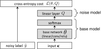
If we know the true noise distribution and it is non-singular, then from Eqn. 7, setting would force to converge to identity. Therefore, training to predict the noisy labels using the combined model parameterized by directly forces the base model to predict the true labels. If the base model is a Convnet network with a softmax output layer, then the noise model is a linear layer, constrained to be a probability matrix, that sits on top of the softmax layer, as shown in Figure 2a. The role of this noise layer is to implement Eqn. 2 on the output of the softmax layer. Therefore, the noise layer is a linear layer with no bias and weights set to matrix . Since this is the only modification to the network, we can still perform back-propagation for training.
3.2 Learning the Noise Distribution
In the previous section, we showed that setting in the noise model is optimal for making the base model accurately predict true labels. In practice, the true noise distribution is often unknown to us. In this case, we have to infer it from the noisy data itself. Fortunately, the noise model is a constrained linear layer in our network, which means its weights can be updated along with other weights in the network. This is done by back-propagating the cross-entropy loss through the matrix, down into the base model. After taking a gradient step with the and the model weights, we project back to the subspace of probability matrices because it represents conditional probabilities.
Unfortunately, simply minimizing the loss in Eqn. 3 will not give us the desired solution. From (3.1), it follows that as the training progresses, where is the confusion matrix of the combined model and is the true noise distribution of data. However, this alone cannot guarantee and . For example, given enough capacity, the base model can start learning the noise distribution and hence , which implies that . Actually, there are infinitely many solutions for where .
In order to force , we add a regularizer on the probability matrix which forces it to diffuse, such as a trace norm or a ridge regression. This regularizer effectively transfers the label noise distribution from the base model to the noise model, encouraging to converge to . Such regularization is reminiscent of blind deconvolution algorithms. Indeed, the noise distribution acts on our system by diffusing the predictions of the base model. When the diffusion kernel is unknown, it is necessary to regularize the ill-posed inverse problem by pushing the estimates away from the trivial identity kernel (Levin et al., 2009).
Under some strong assumptions, we can actually prove that takes the smallest value only when . Let us assume holds true, and and have large diagonal elements (i.e. and for ). Then, it follows
This shows that is a lower bound for , and the equality will hold true only when and . Therefore, minimizing is a sensible way to make the base model accurately predict clean labels. Although the above proof is true under strong assumptions, we show empirically that it works well in practice. Also, we use weight decay on instead of minimizing in practice since it is already implemented in most deep learning packages and has similar effect of diffusing .
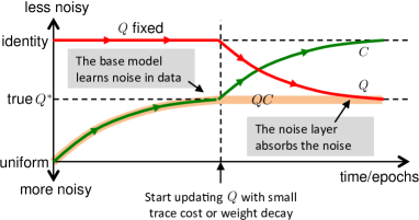
Let us finally describe the learning procedure, illustrated in Figure 2b. In the beginning of training, and are very different in general, and the confusion matrix does not necessarily have large elements on its diagonal. This makes learning difficult. Therefore, we fix at the start of training. This is illustrated in the left part of Figure 2b. At that point, the base model could have learned the noise in the training data (i.e. ), which is not what we want. Therefore, we start updating along with the rest of the network, using weight decay to push away from the identity and towards . As starts to diffuse, it starts absorbing the noise from the base model, thus making the base model more accurate. However, too large weight decay would make more diffused than the true , which may hurt the performance. In case there is no clean data, we cannot tune this weight decay parameters with validation. In the experiments in this paper, we fix the weight decay parameter for to (in some cases where the training classification cost significantly increased because of the weight decay on , we used smaller weight decay parameter). If we want to make prediction or test the model on clear data, the noise layer should be removed (or set to identity ).
3.3 Outlier Noise
Another important setting is the case where some training samples do not belong to any of the existing signal classes. In that case, we can create an additional “outlier” class, which enables us to apply the previously described noise model.
Let be the number of the existing classes. Then, the base network should output probabilities now, where the last one represents the probability of a sample being an outlier. If the labels given to outlier samples are uniformly distributed across classes, then the corresponding noise distribution becomes a matrix
| (8) |
Unfortunately, this matrix is singular and would map two different network outputs and to the exact same point. A simple solution to this problem is to add some extra outlier images with label in the training data, which would make non-singular (in most cases, it is cheap to obtain such extra outlier samples). Now, the noise distribution becomes
| (9) |
Note that in this setting there is no learning: matrix is fixed to given in Eqn. 9. The fraction of outliers in the training set, required to compute , is a hyper-parameter that must be set manually (since there is no principled way to estimate it). However, we experimentally demonstrate that the algorithm is not sensitive to the exact value.
4 Experiments
In this section, we empirically examine the robustness of deep networks with and without noise modeling. First, we perform controlled experiments by deliberately adding two types of label noise to clean datasets: label flip noise and outlier noise. Then we show more realistic experiments using two datasets with inherent label noise, where we do not know the true distribution of noisy labels.
4.1 Data and Model Architecture
We use three different image classification datasets in our experiments. The first dataset is the Google street-view house number dataset (SVHN) (Netzer et al., 2011), which consists of 32x32 images of house number digits captured from Google Streetview. It has about 600k images for training and 26k images for testing. The second one is more challenging dataset CIFAR10 (Krizhevsky & Hinton, 2009), a subset of 80 million Tiny Images dataset (Torralba et al., 2008) of 32x32 natural images labeled into 10 object categories. There are 50k training images and 10k test images. The last dataset is ImageNet (Deng et al., 2009), a large scale dataset of 1.2M images, labeled with 1000 classes. For all datasets, the only preprocessing step is mean subtraction, except for SVHN where we also perform contrast normalization. For ImageNet, we use data augmentation by taking random crop of 227x227 at random locations, as well as horizontal flips with probability 0.5.
For SVHN and CIFAR-10 we use the model architecture and hyperparameter settings given by the CudaConv (Krizhevsky, 2012) configuration file layers-18pct.cfg, which implements a network with three convolutional layers. These settings were kept fixed for all experiments using these datasets. For ImageNet, we use the model architecture described in Krizhevsky et al. (2012) (AlexNet).
4.2 Label Flip Noise
We synthesize noisy data from clean data by stochastically changing some
of the labels: an original label is randomly changed to with
fixed probability . Figure 3c shows the noise distribution
used in our experiments. We can alter this distribution
by changing the probability on the diagonal to generate datasets
with different overall noise levels. The labels of test images are left
unperturbed.
SVHN:
When training a noise model with SVHN data, we fix to the
identity for the first five epochs. Thereafter, is updated
with weight decay 0.1 for 95
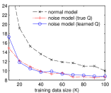
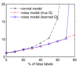
epochs. Figure 3a and 3b shows the test errors for
different training set sizes and different noise levels. These plots
show the normal model coping with up to 30 noise, but then
degrading badly. By contrast, the addition of our noise layer allows
the model to operate with up to 70. Beyond this, the method breaks
down as the false labels overwhelm the correct ones. Overall, the
addition of the noise model consistently achieves better accuracy,
compared with a normal deep network. The figure also shows error rates for
a noise model trained using the true noise distribution . We see
that it performs as well as the learned , showing that our
proposed method for learning the noise distribution from data is
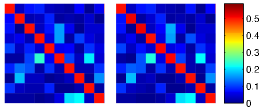
effective. Figure 3c shows an example of a learned
alongside the ground truth used to generate the noisy data. We
can see that the difference between them is negligible.
| Without noise model | With learned noise model | Without noise model | With learned noise model |
 |
 |
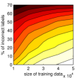 |
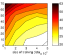 |
| (a) SVHN | (b) CIFAR10 | ||
Figure 4a shows the effects of label flip noise in more detail. The color in the figure shows the test errors (brighter means better), and the contour lines indicates the same accuracy. Without the noise model, the performance drops quickly as the number of incorrect labels increases. In contrast, the convnet with the noise model shows greater robustness to incorrect labels.
CIFAR-10: We perform the same experiments as for SVHN on the CIFAR-10 dataset, varying the training data size and noise level. We fix to identity for the first 30 epochs of training and then run for another 70 epochs updating with weight decay 0.1. The results are shown in Figure 4b. Again, using the noise model is more robust to label noise, compared to the unmodified model. The difference is especially large for high noise levels and large training sets, which shows the scalability of the noise model.
ImageNet: In this experiment, we deliberately flip half of the training labels in ImageNet dataset to test the scalability of our noise model to a 1000 class problem. We explore two different noise distributions: (i) random and (ii) adversarial, applied to the ImageNet 2012 training set. In the random case, labels are flipped with a non-uniform probability using a pre-defined matrix , which has around 10 thousand non-zero values at random off-diagonal locations. I.e for each class, 50% of the labels are correct, with the other 50% being distributed over 10 other randomly chosen classes. In the adversarial case, we use a noise distribution where labels are changed to other classes that are more likely to be confused with the true class (e.g. simulating human mislabeling). First, we train a normal convnet on clean data and measure its confusion matrix. This matrix gives us a good metric of which classes more likely to be confused. Then this matrix is used for constructing so that 40% of labels are randomly flipped to other similar labels.
Using the AlexNet architecture (Krizhevsky et al., 2012), we train three models for each noise case: (i) a standard model with no noise layer; (ii) a model with a learned matrix and (iii) a model with fixed to the ground truth .
Table 1a shows top-1 classification error on the ImageNet 2012 validation set for models trained on the random noise distribution. It is clear that the noise hurts performance significantly. The model with learned shows a clear gain (8.5%) over the unaltered model, but is still 3.8% behind the model that used the ground truth . The learned model is superior to training an unaltered model on the subset of clean labels, showing that the noisy examples carry useful information that can be accessed by our model. Table 1b shows errors for the adversarial noise situation. Here, the overall performance is worse (despite a lower noise level than Table 1a, but the learned noise model is still superior to the unaltered model.
| Noise model | Training size | Noise % | Valid. Error |
|---|---|---|---|
| None | 1.2M | 0 | 39.8% |
| None | 0.6M | 0 | 48.5% |
| None | 1.2M | 50 | 53.7% |
| Learned | 1.2M | 50 | 45.2% |
| True | 1.2M | 50 | 41.4% |
| Noise model | Training size | Noise % | Valid. error |
|---|---|---|---|
| None | 1.2M | 40 | 50.5% |
| Learned | 1.2M | 40 | 46.7% |
| True | 1.2M | 40 | 43.3% |
4.3 Outlier Noise
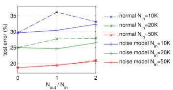
CIFAR-10: Here, we simulate outlier noise by deliberately polluting CIFAR10 training data with randomly chosen images from the Tiny Images dataset (Torralba et al., 2008). Those random images can be considered as outliers because Tiny Images dataset covers 75,000 classes, thus the chance of belonging to 10 CIFAR classes is very small. Our training data consists of a random mix of inlier images with true labels and outlier images with random labels (n.b. the model has no knowledge of which are which). As described in Section 3.3, the outlier model requires a small set of known outlier images. In this case, we use 10k examples randomly picked from Tiny Images. For testing, we use the original (clean) CIFAR10 test data.
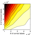
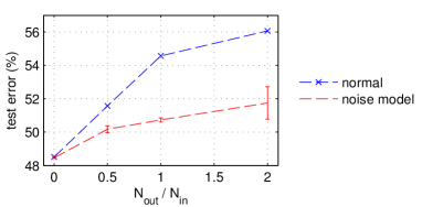
Figure 5(left) shows the classification performance of a model trained on different amounts of inlier and outlier images. Interestingly, a large amount of outlier noise does not significantly reduce the accuracy of the normal model without any noise modeling. Nevertheless, when the noise model is used the effect of outlier noise is reduced, particularly for small training sets. In this experiment, we set hyper-parameter in Eqn. 9 using the true number of outliers but, as shown in Fig. 6, model is not sensitive to the precise value.
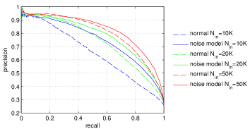
Figure 5(right) explores the ability of the trained models to distinguish inlier from outlier in a held-out noisy test set. For the normal model, we use the entropy of the softmax output as a proxy for outlier confidence. For our outlier model, we use the confidence of the class output. The figure shows precision recall curves for both models trained varying training set sizes with 50% outliers. The average precision for the outlier model is consistently superior to the normal model.
ImageNet: We added outlier noise to ImageNet dataset (1.2M images, 1K categories) using images randomly chosen from the entire ImageNet Fall 2011 release (15M images, 22K categories). Each outlier images is randomly labeled as one of 1K categories and added to the training set.
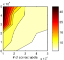
We fix the number of inlier images to be (half of the original ImageNet training data). We increase the number of outlier images up to , mixed into the training data. For training the noise model, we added 20K outlier images, labeled as outlier to the training data. We trained a normal AlexNet model on the data, along with a version using the outlier model. We used three different values (see Eqn. 9) in these experiments. One run used set using the true percentage of outliers in the training data. The other two runs perturbed this value by , to explore the sensitivity of the noise model to this hyper-parameter. The results are shown in Fig. 6 (the error bars show ) for differing amounts of outliers. Although the normal deep network is quite robust to large outlier noise, using the noise model further reduces the effect of noise.
4.4 Real Label Noise
Tiny Images: The Tiny Images dataset (Torralba et al., 2008) is a realistic source of noisily labeled data, having been gathered from Internet search engines. We apply our outlier model to a 200k subset, taken from the 10 classes from which the CIFAR-10 dataset was extracted. The data contains a mix of inlier images, as well as totally unrelated outlier images. After a cursory examination of the data, we estimated the outlier fraction to be . Using this ratio, along with 5k known outliers (randomly drawn Tiny Images), was set to . For evaluation we used the CIFAR-10 test set111We carefully removed from the training set any images that were present in the CIFAR-10 test set.. Training on this data using an unmodified convnet produced a test error of 19.2%. A second model, trained with an outlier layer, gave a test error of 18.8%, a relative gain of 2.1%.
Web Images + ImageNet: We also apply our approach to a more challenging noisy real world problem based around the 1000 classes used in ImageNet. We collected a new noisy web image dataset, using each of the thousand category names as input into Internet image search engines. All available images for each class were downloaded, taking care to delete any that also appeared in the ImageNet dataset. This dataset averages 900 examples/class for a total of 0.9M images. The noise is low for the highly ranked images, but significant for the later examples of each class. The precise noise level is unknown, but after browsing some of the images we set , assuming 20% of images are outlier. We trained an AlexNet model (Krizhevsky et al., 2012) with and without the noise adaption layer on this web image dataset and evaluated the performance on the ImageNet 2012 validation set. One complication is that the distribution of inliers in the web images differs somewhat from the ImageNet evaluation set, creating a problem of domain shift. To reduce this effect (so that the noise adaptation effects of our approach can be fairly tested), we added 0.3M ImageNet training images to our web data. This ensures that the model learns a representation for each class that is consistent with the test data.
Table 2 shows three Alexnet models applied to the data: (i) an unaltered model, (ii) a model with learned label-flip noise matrix (weigh decay parameter for set to 0.02 because larger value significantly increased the training classification cost) and (iii) a model with an outlier noise matrix (with set to 0.08). The results show the label-flip model boosting performance by 0.6%.
| Method | Valid. error |
|---|---|
| Normal Convnet | 48.8% |
| Label-flip model | 48.2% |
| Outlier model | 48.5% |
5 Conclusion
In this paper we explored how convolutional networks can be trained on data with noisy labels. We proposed two simple models for improving noise robustness, focusing different types of noise. We explored both approaches in a variety of settings: small and large-scale datasets, as well as synthesized and real label noise. In the former case, both approaches gave significant performance gains over a standard model. On real data, then gains were smaller. However, both approaches can be implemented with minimal effort in existing deep learning implementations, so add little overhead to any training procedure.
References
- Barandela & Gasca (2000) Barandela, Ricardo and Gasca, Eduardo. Decontamination of training samples for supervised pattern recognition methods. In Advances in Pattern Recognition, volume 1876 of Lecture Notes in Computer Science, pp. 621–630. Springer, 2000.
- Bootkrajang & Kab n (2012) Bootkrajang, Jakramate and Kab n, Ata. Label-noise robust logistic regression and its applications. In Machine Learning and Knowledge Discovery in Databases, volume 7523 of Lecture Notes in Computer Science, pp. 143–158. Springer, 2012.
- Brodley & Friedl (1999) Brodley, Carla E. and Friedl, Mark A. Identifying mislabeled training data. Journal of Artificial Intelligence Research, 11:131–167, 1999.
- Collobert et al. (2011) Collobert, Ronan, Kavukcuoglu, Koray, and Farabet, Clément. Torch7: A matlab-like environment for machine learning. In BigLearn, NIPS Workshop, 2011.
- Deng et al. (2009) Deng, Jia, Dong, Wei, Socher, R., Li, Li-Jia, Li, Kai, and Fei-Fei, Li. Imagenet: A large-scale hierarchical image database. In Computer Vision and Pattern Recognition, 2009. CVPR 2009. IEEE Conference on, pp. 248–255, June 2009.
- Erhan et al. (2010) Erhan, Dumitru, Bengio, Yoshua, Courville, Aaron, Manzagol, Pierre-Antoine, Vincent, Pascal, and Bengio, Samy. Why does unsupervised pre-training help deep learning? J. Mach. Learn. Res., 11:625–660, March 2010.
- Fergus et al. (2009) Fergus, Rob, Weiss, Yair, and Torralba, Antonio. Semi-supervised learning in gigantic image collections. In Bengio, Y., Schuurmans, D., Lafferty, J.D., Williams, C.K.I., and Culotta, A. (eds.), Advances in Neural Information Processing Systems 22, pp. 522–530. 2009.
- Frenay & Verleysen (2014) Frenay, B. and Verleysen, M. Classification in the presence of label noise: A survey. Neural Networks and Learning Systems, IEEE Transactions on, 25(5):845–869, May 2014.
- Guyon et al. (1996) Guyon, Isabelle, Matic, Nada, and Vapnik, Vladimir. Discovering informative patterns and data cleaning. In Advances in Knowledge Discovery and Data Mining, pp. 181–203. 1996.
- Hinton & Salakhutdinov (2006) Hinton, G. E. and Salakhutdinov, R. R. Reducing the dimensionality of data with neural networks. Science, 313(5786):504–507, 2006.
- Ipeirotis et al. (2010) Ipeirotis, Panagiotis G., Provost, Foster, and Wang, Jing. Quality management on amazon mechanical turk. In Proceedings of the ACM SIGKDD Workshop on Human Computation, HCOMP ’10, pp. 64–67. ACM, 2010.
- Jia et al. (2014) Jia, Yangqing, Shelhamer, Evan, Donahue, Jeff, Karayev, Sergey, Long, Jonathan, Girshick, Ross, Guadarrama, Sergio, and Darrell, Trevor. Caffe: Convolutional architecture for fast feature embedding. arXiv preprint arXiv:1408.5093, 2014.
- Krizhevsky (2012) Krizhevsky, Alex. cuda-convnet. https://code.google.com/p/cuda-convnet/, 2012.
- Krizhevsky & Hinton (2009) Krizhevsky, Alex and Hinton, Geoffrey. Learning multiple layers of features from tiny images. Computer Science Department, University of Toronto, Tech. Rep, 2009.
- Krizhevsky et al. (2012) Krizhevsky, Alex, Sutskever, Ilya, and Hinton, Geoffrey E. Imagenet classification with deep convolutional neural networks. In Advances in Neural Information Processing Systems 25, pp. 1097–1105, 2012.
- Larsen et al. (1998) Larsen, J., Nonboe, L., Hintz-Madsen, M., and Hansen, L.K. Design of robust neural network classifiers. In Acoustics, Speech and Signal Processing, 1998. Proceedings of the 1998 IEEE International Conference on, volume 2, pp. 1205–1208 vol.2, May 1998.
- Le (2013) Le, Q.V. Building high-level features using large scale unsupervised learning. In Acoustics, Speech and Signal Processing (ICASSP), 2013 IEEE International Conference on, pp. 8595–8598, May 2013.
- LeCun et al. (1989) LeCun, Y., Boser, B., Denker, J. S., Henderson, D., Howard, R. E., Hubbard, W., and Jackel, L. D. Backpropagation applied to handwritten zip code recognition. Neural Computation, 1(4):541–551, 2014/11/13 1989.
- Lecun et al. (1998) Lecun, Y., Bottou, L., Bengio, Y., and Haffner, P. Gradient-based learning applied to document recognition. Proceedings of the IEEE, 86(11):2278–2324, Nov 1998.
- Lee et al. (2009) Lee, Honglak, Grosse, Roger, Ranganath, Rajesh, and Ng, Andrew Y. Convolutional deep belief networks for scalable unsupervised learning of hierarchical representations. In Proceedings of the 26th Annual International Conference on Machine Learning, ICML ’09, pp. 609–616. ACM, 2009.
- Levin et al. (2009) Levin, A., Weiss, Y., Durand, F., and Freeman, W. T. Understanding and evaluating blind deconvolution algorithms. In CVPR, 2009.
- Mnih & Hinton (2012) Mnih, Volodymyr and Hinton, Geoffrey. Learning to label aerial images from noisy data. In Proceedings of the 29th International Conference on Machine Learning (ICML-12), pp. 567–574, 2012.
- Natarajan et al. (2013) Natarajan, Nagarajan, Dhillon, Inderjit, Ravikumar, Pradeep, and Tewari, Ambuj. Learning with noisy labels. In Advances in Neural Information Processing Systems 26, pp. 1196–1204. 2013.
- Nettleton et al. (2010) Nettleton, David, Orriols-Puig, Albert, and Fornells, Albert. A study of the effect of different types of noise on the precision of supervised learning techniques. Artificial Intelligence Review, 33(4):275–306, 2010.
- Netzer et al. (2011) Netzer, Yuval, Wang, Tao, Coates, Adam, Bissacco, Alessandro, Wu, Bo, and Ng, Andrew Y. Reading digits in natural images with unsupervised feature learning. In NIPS Workshop on Deep Learning and Unsupervised Feature Learning, 2011.
- Pechenizkiy et al. (2006) Pechenizkiy, M., Tsymbal, A., Puuronen, S., and Pechenizkiy, O. Class noise and supervised learning in medical domains: The effect of feature extraction. In Computer-Based Medical Systems, 2006. CBMS 2006. 19th IEEE International Symposium on, pp. 708–713, 2006.
- Sermanet et al. (2014) Sermanet, Pierre, Eigen, David, Zhang, Xiang, Mathieu, Michael, Fergus, Rob, and LeCun, Yann. Overfeat: Integrated recognition, localization and detection using convolutional networks. In International Conference on Learning Representations (ICLR 2014), April 2014.
- Simonyan & Zisserman (2014) Simonyan, Karen and Zisserman, Andrew. Very deep convolutional networks for large-scale image recognition. arXiv preprint arXiv:1409.1556, 2014.
- Taigman et al. (2014) Taigman, Yaniv, Yang, Ming, Ranzato, Marc’Aurelio, and Wolf, Lior. DeepFace: Closing the Gap to Human-Level Performance in Face Verification. Conference on Computer Vision and Pattern Recognition (CVPR), 2014.
- Talwalkar et al. (2008) Talwalkar, A., Kumar, S., and Rowley, H. Large-scale manifold learning. In CVPR, 2008.
- Torralba et al. (2008) Torralba, A., Fergus, R., and Freeman, W.T. 80 million tiny images: A large data set for nonparametric object and scene recognition. Pattern Analysis and Machine Intelligence, IEEE Transactions on, 30(11):1958–1970, Nov 2008.
- van den Hout & van der Heijden (2002) van den Hout, Ardo and van der Heijden, Peter G.M. Randomized response, statistical disclosure control and misclassificatio: a review. International Statistical Review, 70(2):269–288, 2002.
- Zhou et al. (2004) Zhou, D., Bousquet, O., Lal, T., Weston, J., and Scholkopf, B. Learning with local and global consistency. In NIPS, 2004.
- Zhu & Lafferty (2005) Zhu, X. and Lafferty, J. Harmonic mixtures: combining mixture models and graph-based methods for inductive and scalable semi-supervised learning. In ICML, 2005.
- Zhu et al. (2003) Zhu, X., Ghahramani, Z., and Laffery, J. Semi-supervised learning using gaussian fields and harmonic functions. In ICML, 2003.
- Zhu (2008) Zhu, Xiaojin. Semi-supervised learning literature survey. In Computer Sciences TR 1530, University of Wisconsin Madison, 2008.
- Zhu & Wu (2004) Zhu, Xingquan and Wu, Xindong. Class noise vs. attribute noise: A quantitative study. Artificial Intelligence Review, 22(3):177–210, 2004.