MeGARA: Menu-based Game Abstraction and
Abstraction Refinement of Markov Automata

Abstract

Markov automata combine continuous time, probabilistic transitions, and nondeterminism in a single model. They represent an important and powerful way to model a wide range of complex real-life systems. However, such models tend to be large and difficult to handle, making abstraction and abstraction refinement necessary. In this paper we present an abstraction and abstraction refinement technique for Markov automata, based on the game-based and menu-based abstraction of probabilistic automata. First experiments show that a significant reduction in size is possible using abstraction.

1 Introduction

Markov automata (MA) constitute a compositional behavioural model for continuous-time stochastic and nondeterministic systems [11, 10, 7]. MA are on one hand rooted in continuous-time Markov chains (CTMCs) and on the other hand based on probabilistic automata (PA) [23]. MA have seen applications in diverse areas where exponentially distributed delays are intertwined with instantaneous random switching. The latter enables MA to capture the complete semantics [9] of generalised stochastic Petri nets (GSPNs) [20] and of stochastic activity networks (SANs) [21]. As MA extend Hermanns’ interactive Markov chains (IMCs) [18], they inherit IMC application domains, ranging from GALS hardware designs [5] and dynamic fault trees [3] to the standardised modelling language AADL [4, 17]. Due to these attractive semantic and compositionality features, there is a growing interest in modelling and analysis techniques for MA.

The semantics of MA including weak and strong (bi)simulation has been studied in [11, 10, 7]. Markov automata process algebra (MAPA) [25] supports fully compositional construction of MA equipped with some minimisation techniques. Analysis algorithms for expected reachability time, long-run average, and timed (interval) reachability have been studied in [15]. It is also accompanied by a tool chain that supports modelling and reduction of MA using SCOOP [25] and analysis of the aforementioned objectives using IMCA [13]. Model checking of MA with respect to continuous stochastic logic (CSL) has been presented in [16].

The core complexity of MA model checking lies in the model checking of time-bounded until formulae. The property is reducible to timed reachability computation where the maximum and minimum probability of reaching a set of target states within a time bound is asked for. The current trend inspired by [22, 29] is to split the time horizon into equally sized discretisation steps, each small enough such that with high probability at most one Markov transition occurs in any step. However, the practical efficiency and accuracy of this approach turns out to be substantially inferior to the one known for CTMCs, and this limits the applicability to real industrial cases. It can only scale up to models with a few thousand states, depending on the parameters of the model and the time bound under consideration. This paper proposes an abstraction refinement technique to address the scalability problem of model checking time-bounded until for MA.

Abstraction refinement methods have gained popularity as an effective technique to tackle scalability problems (e. g. state space explosion) in probabilistic and non-probabilistic settings. Although abstraction refinement techniques have not been employed for MA yet, there are a number of related works on PA, which allow to estimate lower and/or upper bounds of reachability probabilities. PA-based abstraction [6] abstracts the concrete model into a PA, which provides an upper bound for maximal and a lower bound for minimal reachability of the concrete model. Game-based abstraction [19] on the other hand enables to compute both lower and upper bound on reachability, i. e. the reachability probability in PA is guaranteed to lie in a probability interval resulting from the analysis of the abstract model, which is represented by a game. This further has been proven to be the best transformer [28]. In this work we nevertheless employ menu-based abstraction [27], which can be exponentially smaller in the size of transitions and also easier to implement. Moreover it provides lower and upper bounds on reachability like game-based abstraction.

In this paper we introduce a menu-based game abstraction refinement approach which generalises Wachter’s method [27] to MA and combines it with Kattenbelt’s method [19]. As mentioned before, the essential part of CSL model checking reduces to timed reachability computation. We accordingly focus on this class of properties. We exploit scheduler-based refinement which splits an abstract block by comparing the decisions made by the lower and upper bound schedulers. Furthermore, we equip the refinement procedure with a pseudo-metric that measures how close a scheduler is to the optimal one. It turns out that the latter enhances the splitting procedure to be coarser. We start the computation with a relatively low precision and increase it repeatedly, thus speeding up the refinement procedure in the beginning while ensuring a high quality of the final abstraction. Our experiments show promising results, especially we can report on a significant compaction of the state space.

Organisation of the paper. At first we give a brief introduction into the foundations of MA and stochastic games in Section 2. Afterwards we will present our approach for the menu-based game abstraction of MA, its analysis and subsequent refinement in Section 3. Experimental results will be shown in Section 4. Section 5 concludes the paper and gives an outlook to future work.

2 Foundations

In this section we will take a brief look at the basics of MA and continuous-time stochastic games.

2.1 Markov Automata

We denote the real numbers by $\mathbb{R}$, the non-negative real numbers by $\mathbb{R}_{\geq 0}$, and by $\mathbb{R}_{\geq 0}^{\infty}$ the set $\mathbb{R}_{\geq 0}\cup\{\infty\}$. For a finite or countable set $S$ let $\text{Distr}(S)$ denote the set of probability distributions on $S$, i. e. of all functions $\mu:S\to[0,1]$ with $\sum_{s\in S}\mu(s)=1$. A rate distribution on $S$ is a function $\rho:S\to\mathbb{R}_{\geq 0}$. The set of all rate distributions on $S$ is denoted by $\text{RDistr}(S)$.

Definition 1 (Markov automaton)

A Markov automaton (MA) $\mathcal{M}=(S,s_{0},A,\mathbf{P},R)$ consists of a finite set $S$ of states with $s_{0}\in S$ being the initial state, a finite set $A$ of actions, a probabilistic transition relation $\mathbf{P}\subseteq S\times A\times\text{Distr}(S)$, and a Markov transition relation $R:S\to\text{RDistr}(S)$.

The rate $R(s)(s^{\prime})$ is the parameter of an exponential distribution governing the time at which the transition from state $s$ to state $s^{\prime}$ becomes enabled. The probability that this happens within time $t$ is given by $1-e^{-R(s)(s^{\prime})\cdot t}$.

We make the usual assumption that we have a closed system, i. e. all relevant aspects have already been integrated into the model such that no further interaction with other components occurs. Then nothing prevents probabilistic transitions from being executed immediately. This is called the maximal progress assumption [7]. Since the probability that a Markov transition becomes enabled immediately is zero, we may assume that a state has either probabilistic or Markov transitions. We denote the set of states with Markov transitions as $\mathit{MS}$. $\mathit{PS}$ is the set of states with probabilistic transitions. It holds that $\mathit{MS}\cap\mathit{PS}=\emptyset$.

If there is more than one Markov transition leaving $s\in\mathit{MS}$ a race condition occurs [7]: The first transition that becomes enabled is taken. We define the exit rate $\mathbf{E}(s)=\sum_{s^{\prime}\in S}R(s)(s^{\prime})$ of state $s\in\mathit{MS}$.

Starting in the initial state $s_{0}$, a run of the system is generated as follows: If the current state $s\in\mathit{MS}$ is Markovian, the sojourn time is determined according to the continuous probability distribution $(1-e^{-\mathbf{E}(s)t})$. At this point in time a transition to $s^{\prime}\in S$ occurs with probability $\frac{R(s)(s^{\prime})}{\mathbf{E}(s)}$. Taking this together, the probability that a transition from $s\in\mathit{MS}$ to $s^{\prime}$ occurs within time $t\geq 0$ is

$$\mu(s)(s^{\prime},t)=(1-e^{-\mathbf{E}(s)t})\frac{R(s)(s^{\prime})}{\mathbf{E}(s)}\ .$$

In a probabilistic state $s\in\mathit{PS}$ first a transition $(s,\alpha,\mu)\in\mathbf{P}$ is chosen nondeterministically. Then the probability to go from $s$ to successor state $s^{\prime}\in S$ is given by $\mu(s^{\prime})$. The sojourn time in probabilistic states is 0.

The nondeterminism between the probabilistic transitions in state $s$ is resolved through a scheduler. The most general scheduler class maps the complete history up to the current probabilistic state to the set of transitions enabled in that state. Considering the general scheduler class is extremely excessive for most objectives like time-bounded reachability, for which a simpler class, namely total-time positional deterministic schedulers suffice [22]. Schedulers of this class resolve nondeterminism by picking an action of the current state, which is probabilistic, based on the total time that has elapsed. Formally, it is a function $\sigma:\mathit{PS}\times\mathbb{R}_{\geq 0}\rightarrow A\times\text{Distr}(S)$ with $\sigma(s,t)=(\alpha,\mu)$ only if $(s,\alpha,\mu)\in\mathbf{P}$.

Time-bounded reachability in MA quantifies the minimum and the maximum probability to reach a set of target states within a given time interval. A fixed point characterisation is proposed in [16] to compute this objective. The characterisation is, however, in general not algorithmically tractable [2]. To circumvent this problem, the fixed point characterisation is approximated by a discretisation approach [16]. Intuitively, the time horizon is divided into equally sized sub-intervals, each one of length $\delta>0$. Discretisation step $\delta$ is presumed to be small enough such that, with high probability, at most one Markov transition fires within time $\delta$. This assumption discretises an MA by summarising its behaviour at equidistant time points. Time-bounded reachability is then computed on the discretised model, together with a stable error bound. The whole machinery is here generalised to stochastic games and the algorithm is later employed to establish a lower and an upper bound for both minimal and maximal time-bounded reachability probabilities in MA.

The MA we consider are non-Zeno, i. e. they do not have any end components consisting only of probabilistic states. Otherwise it would be possible to have an infinite amount of transitions taking place in a finite amount of time.

For more on MA in general we recommend [7].

2.2 Stochastic Games

Stochastic games are generalisations of MA. They also combine continuous time with nondeterminism and probabilities.

A stochastic game consists of one or several players who can choose between one or several actions. In turn, these actions may influence the behaviour of the other players. Each action consists of a real-valued or infinite rate $\lambda\in\mathbb{R}_{\geq 0}^{\infty}$ and a probability distribution. For our work we need the definition of two-player games:

Definition 2 (Stochastic game)

A stochastic continuous-time two-player game is a tuple $\mathcal{G}=(V,(V_{1},V_{2}),$ $v_{0},A,T)$ such that $V=V_{1}\mathbin{\dot{\cup}}V_{2}$ is a set of states, $v_{0}\in V$ is the initial state, $A$ is a finite set of actions and $T\subseteq V\times A\times\mathbb{R}_{\geq 0}^{\infty}\times\text{Distr}(V)$ is a probabilistic transition relation with continuous time.

$V_{1}$ and $V_{2}$ are the states of player 1 and player 2, respectively. We define two functions $\theta_{p}:T\to\text{Distr}(V)$ and $\theta_{r}:T\to\mathbb{R}_{\geq 0}^{\infty}$. $\theta_{p}$ is a projection on the probability distribution of a transition, $\theta_{r}$ is a projection on the rate. If the current state is $v\in V_{1}$, then it is player 1’s turn to choose the next transition, otherwise player 2’s. The current player chooses a transition $(v,\alpha,\lambda,\mu)\in T$ for leaving state $v$. $\theta_{r}(v,\alpha,\lambda,\mu)=\lambda\in\mathbb{R}_{\geq 0}^{\infty}$ determines how long this action takes, whereas $\theta_{p}(v,\alpha,\lambda,\mu)=\mu\in\text{Distr}(V)$ gives us the distribution which leads to a successor state. A typical goal of such games is, e. g., that player 1 wants to reach a goal state within a given time bound and player 2 tries to prevent this.

In the following we denote states of player 1 and player 2 as $V_{1}$-states and $V_{2}$-states.

The nondeterminism which may occur at a certain player state is resolved by a scheduler, which is in this case called a strategy. Each player follows his own strategy in order to accomplish its goal. As for MA, total-time positional deterministic strategies are sufficient since we are concentrating on time-bounded reachability. A strategy for player $x\in\{1,2\}$ is therefore defined as a function $\sigma_{x}:V_{x}\times\mathbb{R}_{\geq 0}\to A\times\mathbb{R}_{\geq 0}^{\infty}\times\text{Distr}(V)$, with $\sigma_{x}(v,t)=(\alpha,\lambda,\mu)$ only if $(v,\alpha,\lambda,\mu)\in T$. Depending on their strategies, players may co-operate or compete with each other.

With the strategies of both players in place, the nondeterminism within a stochastic game is resolved, the result being a deterministic MA. Stochastic games with strategies therefore have the same semantics as MA, especially the discretisation of continuous-time stochastic games works in a similar way.

For more on strategies and on stochastic games in general we refer to [24].

3 Abstraction, Analysis and Refinement

Abstraction in general is based on a partition $\mathcal{P}=\{B_{1},B_{2},\ldots,B_{n}\}$ of the state space. The original or concrete states are lumped together into abstract states, defined by the blocks $B_{i}\in\mathcal{P}$.

For PA, both game- and menu-based abstraction use these blocks $B_{i}$ as player 1 states (i. e. $V_{1}=\mathcal{P}$). In game-based abstraction [19] for PA player 2 states in $V_{2}$ represent sets of concrete states that have the same branching structure. In menu-based abstraction [27] the states of player 2 represent the set of enabled actions within a block $B_{i}$. Abstraction refinement for both approaches is based on values and schedulers which are computed for certain properties.

MA are an extension of PA, they additionally contain Markov transitions. In our work we aspire to transfer the results of [19] and [27] from PA to MA. Menu-based abstraction [27] is usually more compact than game-based abstraction [19], since in general there are more different states within a block than different enabled actions. However, the game-based abstraction is more suitable for Markovian states as Markov transitions are not labelled with actions. Therefore we decided to combine both techniques, which is described in the following section.

For the remainder of the paper we define $A(B)=\{\alpha\in A\,|\,\exists s\in B\ \exists\mu\in\text{Distr}(S):(s,\alpha,\mu)\in\mathbf{P}\}$ as the set of actions which are enabled within a set of states $B\subseteq S$.

3.1 Menu-based Game Abstraction for MA

As in the case of [19, 27], our menu-based game abstraction is based on a partition $\mathcal{P}$. Each block of $\mathcal{P}$ either contains probabilistic or Markovian states, not both. It holds that $B_{i}\cap B_{j}=\emptyset$ for all $i,j\in\{1\ldots,n\}$.

The probabilistic blocks of partition $\mathcal{P}$ constitute the $V_{1}$-states, whereas $V_{2}$-states either represent the enabled actions within a probabilistic block, a Markovian block of $\mathcal{P}$, or the concrete states within a Markovian block. Thus, the original nondeterminism of the MA is represented in the $V_{1}$-states, the nondeterminism artificially introduced by the abstraction is present in $V_{2}$-states.

The transitions of the original MA $\mathcal{M}$ have to be lifted to sets of states as follows:

Definition 3 (Lifted (rate) distribution)

Let $\mu\in\text{Distr}(S)$ be a probability distribution over $S$ and $\mathcal{P}$ a partition of $S$. The lifted distribution $\overline{\mu}\in\text{Distr}(\mathcal{P})$ is given by $\overline{\mu}(B)=\sum_{s\in B}\mu(s)$ for $B\in\mathcal{P}$. Accordingly for a rate distribution $\rho\in\text{RDistr}(S)$ we define $\overline{\rho}\in\text{RDistr}(\mathcal{P})$ by $\overline{\rho}(B)=\sum_{s\in B}\rho(s)$ for all $B\in\mathcal{P}$.

If several probabilistic distributions for an action $\alpha$ within a partition block $B_{i}$ turn out to be the same after lifting, they are unified. Additionally, if action $\alpha\in A(B_{i})$ is not enabled in a state $s\in B_{i}$, then a new probabilistic distribution is added with $\xi_{*}(*)=1.0$, ‘$*$’ being a newly added bottom state. This can be interpreted as the lifting of nonexistent distributions. Example 1 and Figure 1 illustrate the abstraction process for probabilistic states, which is a direct transfer from Wachter’s menu-based abstraction [27].

Figure 1: Example for the menu-based abstraction of probabilistic states.

Example 1

Figure 1 shows a part of an MA $\mathcal{M}$ and a partition $\mathcal{P}$. The probabilistic states ‘$a$’ and ‘$e$’ of $\mathcal{M}$ are contained in the same block $B_{i}$. In the abstraction, which is shown in Figure 1, $B_{i}$ becomes a $V_{1}$-state—indicated as a square—, whereas the actions $\alpha,\beta\in A(B_{i})$ become $V_{2}$-states—indicated as diamonds. Since $\alpha$ is not enabled in the concrete state ‘$e$’, a ‘$*$’-transition is added to the abstract $\alpha$-state.

As can be seen, the original nondeterminism is resolved by the choice of player 1 between the different enabled actions, whereas an introduced nondeterminism is present at player 2. To make the later abstraction refinement easier (s. Section 3.3) we also retain a mapping between the abstract distributions and the corresponding concrete states, as indicated in Figure 1.

For Markovian states, the menu-based approach from [27] cannot be used, since Markov transitions do not have actions which can be used as $V_{2}$-states. This is indicated by using the $\bot$-symbol. Our approach for Markovian states is therefore more similar to Kattenbelt’s game-based abstraction [19]: A Markovian block $B_{i}$ becomes a $V_{2}$-state, succeeded by $V_{2}$-states representing the concrete states within $B_{i}$ which have the same lifted Markov transitions according to Definition 3. In the following, we denote $V_{2}$-states representing a Markovian block (concrete states) as abstract (concrete) Markovian $V_{2}$-states.

Example 2 and Figure 2 demonstrate the abstraction of Markovian states.

Figure 2: Example for the game-based abstraction of Markovian states.

Example 2

Figure 2 shows a part of an MA $\mathcal{M}$. The Markovian states ‘$a$’ and ‘$e$’ of $\mathcal{M}$ are contained in the same block $B_{i}$. $\lambda_{1}$, $\lambda_{2}$ and $\lambda_{3}$ denote the rates of the rate distribution of ‘$a$’.

The block $B_{i}$ becomes an abstract Markovian $V_{2}$-state in the abstraction as shown in Figure 2. The other $V_{2}$-states, however, correspond directly to the concrete states. Since the lifted rate distribution of ‘$a$’ is different from the one of ‘$e$’—not shown here—, the concrete states stay separate, otherwise they would be unified.

It has to be noted, that at abstract Markovian $V_{2}$-states only introduced nondeterminism occurs. In the concrete system there is no nondeterminism here, we have the race condition instead.

All transitions leading from a $V_{1}$-state $v_{1}$ to a $V_{2}$-state $v_{2}$ are considered to be immediate, i. e. they do not require any time. This is symbolised by giving them the rate $R(v_{1})(v_{2})=\infty$. The same holds for transitions leading from abstract Markovian to concrete Markovian $V_{2}$-states and for probabilistic transitions from a probabilistic $V_{2}$-state to a successor state. The nondeterministic transitions from a $V_{1}$- or from an abstract Markovian $V_{2}$- to a $V_{2}$-state $v_{2}$ are associated with the unique probability distribution $\xi_{v_{2}}$ with $\xi_{v_{2}}(v_{2})=1.0$. For a clearer representation we omitted point-distributions $\xi_{v_{2}}$ and rates $\infty$ in the preceding and in the following figures and examples.

We additionally define $[s]_{\mathcal{P}},s\in S$ as the (unique) block $B\in\mathcal{P}$ with $s\in B$.

After these preliminaries we can formally define our menu-based game abstraction of MA.

Definition 4 (Menu-based game abstraction)

Given an MA $\mathcal{M}=(S,s_{0},A,\mathbf{P},R)$ and partition $\mathcal{P}=\{B_{1},\dots B_{n}\}$ of $S$. We construct the menu-based game abstraction $\mathcal{G}_{\mathcal{M}}^{\mathcal{P}}=(V,(V_{1},V_{2}),v_{0},\overline{A},\overline{T})$ with:

• $V=V_{1}\mathbin{\dot{\cup}}V_{2}$,

• $V_{1}=\{v\in\mathcal{P}\,|\,v\subseteq\mathit{PS}\}\mathbin{\dot{\cup}}\{*\}$,

• $V_{2}=\bigl{\{}(v_{1},\alpha)\in\mathcal{P}\times A\,\big{|}\,v_{1}\subseteq\mathit{PS}\land\alpha\in A(v_{1})\bigr{\}}\mathbin{\dot{\cup}}\bigl{\{}v\in\mathcal{P}\,|\,v\subseteq\mathit{MS}\bigr{\}}$
        ${}\mathbin{\dot{\cup}}\bigl{\{}(v_{1},\overline{\rho})\in\mathcal{P}\times\text{RDistr}(\mathcal{P})\,\big{|}\,v_{1}\subseteq\mathit{MS}\land\exists s\in v_{1}:R(s)=\rho\bigr{\}}$,

• $v_{0}=[s_{0}]_{\mathcal{P}}$,

• $\overline{A}=A\mathbin{\dot{\cup}}\{\bot\}$, and

• $\overline{T}\subseteq V\times\overline{A}\times\mathbb{R}_{\geq 0}^{\infty}\times\text{Distr}(V)$ is given by $\overline{T}=\overline{T_{\mathit{PS}}}\mathbin{\dot{\cup}}\overline{T_{\mathit{MS}}}$ with

  $$\overline{T_{\mathit{PS}}} =\bigl{\{}([s]_{\mathcal{P}},\bot,\infty,\xi_{([s]_{\mathcal{P}},\alpha)})\,\big{|}\,s\in\mathit{PS}\land\alpha\in A(s)\bigr{\}}$$

  $$\qquad\cup\bigl{\{}\bigl{(}([s]_{\mathcal{P}},\alpha),\alpha,\infty,\overline{\mu}\bigr{)}\,\big{|}\,s\in\mathit{PS}\land(s,\alpha,\mu)\in P\bigr{\}}$$

  $$\qquad\cup\bigl{\{}\bigl{(}([s]_{\mathcal{P}},\alpha),\bot,\infty,\xi_{\ast}\bigr{)}\,\big{|}\,s\in\mathit{PS}\land\alpha\not\in A(s)\bigr{\}}$$

  $$\overline{T_{\mathit{MS}}} =\bigl{\{}([s]_{\mathcal{P}},\bot,\infty,\xi_{([s]_{\mathcal{P}},\overline{\rho})})\,\big{|}\,s\in\mathit{MS}\land\rho=R(s)\bigr{\}}$$

  $$\qquad\cup\bigl{\{}\bigl{(}([s]_{\mathcal{P}},\overline{\rho}),\bot,\mathbf{E}(s),\frac{\overline{\rho}}{\mathbf{E}(s)}\bigr{)}\,\big{|}\,s\in\mathit{MS}\land\rho=R(s)\bigr{\}}.$$

The probability distributions $\mu\in\text{Distr}(V)$ and rate distributions $\rho\in\text{RDistr}(\mathcal{P})$ are as stated previously. For the remainder of this paper we will not refer to the transition relation $\overline{T}$, but directly to the probabilistic distributions and rate distributions.

Figure 3 and Example 3 illustrate the abstraction process.

Figure 3: An example for the menu-based game abstraction of an MA $\mathcal{M}$.

Example 3

Figure 3 shows an MA $\mathcal{M}$ and a partition $\mathcal{P}=\{B_{0},B_{1},B_{2}\}$. $B_{0}$ contains all Markovian states of $\mathcal{M}$ and $B_{1}$ all probabilistic states, except the goal state $s_{6}$, which is contained in the separate block $B_{2}$. The corresponding menu-based game abstraction $\mathcal{G}_{\mathcal{M}}^{\mathcal{P}}$ is pictured in Figure 3.

As can be seen, $B_{0}$ becomes an abstract Markovian $V_{2}$-state, whereas the blocks $B_{1}$ and $B_{2}$ build the $V_{1}$-states of $\mathcal{G}_{\mathcal{M}}^{\mathcal{P}}$. The abstract Markovian state $B_{0}$ leads to a set of $V_{2}$-states, which either correspond directly to concrete states (in the case of ‘$s_{0}$’ and ‘$s_{1}$’) or to a set of concrete states (in the case of ‘$s_{3},s_{5}$’). The abstract Markovian $V_{2}$-state $B_{0}$ is also the initial state of $\mathcal{G}_{\mathcal{M}}^{\mathcal{P}}$, since the block contains the concrete initial state $s_{0}$.

The only enabled action within block $B_{1}$ is $\alpha$, the same holds for $B_{2}$. The corresponding abstract states lead each to a $V_{2}$-state labelled with $\alpha$. Although $B_{1}$ contains two probabilistic states, $s_{2}$ and $s_{4}$, only one distribution goes out from the respective $\alpha$-state, since the distributions after lifting are identical.

3.2 Analysis of the Abstraction

As mentioned before, there are two kinds of nondeterminism present in the abstraction: the original, concrete nondeterminism and the introduced abstract one. As in [19, 27] the nondeterministic choices are resolved by two separate schedulers: the concrete scheduler $\sigma_{c}:V_{1}\times\mathbb{R}_{\geq 0}\to\overline{T}$ of player 1 and the abstract scheduler $\sigma_{a}:V_{2}\times\mathbb{R}_{\geq 0}\to\overline{T}$ of player 2. These schedulers are total-time positional deterministic strategies of stochastic games (see Section 2.2).

For Markovian blocks only the abstract scheduler $\sigma_{a}$ exists, since only the introduced nondeterminism is present there. This can be seen in Figure 2: A (nondeterministic) choice occurs at the abstract Markovian $V_{2}$-state only, whereas there is no choice for the concrete Markovian $V_{2}$-states.

While the concrete scheduler $\sigma_{c}$ always behaves according to the property under consideration, e. g. in case of maximal bounded reachability $\sigma_{c}$ tries to maximise the result, the abstract scheduler $\sigma_{a}$ can either co-operate or compete with $\sigma_{c}$, i. e. it can try to maximise or minimise the probability. This leads to the existence of an upper and a lower bound for every property. The value of the original system lies within these bounds. We omit the proof of this for now, however it is similar to the proof of the correctness of the menu-based or game-based abstraction of PA in [19] or in [27].

If the bounds are too far apart, the abstraction is too coarse and has to be refined (s. Section 3.3).

As already mentioned, we are currently concentrating on time-bounded reachability, but we are going to consider a wider set of properties in the future.

3.2.1 Time-bounded Reachability

If we want to analyse a property within the abstraction $\mathcal{G}_{\mathcal{M}}^{\mathcal{P}}$, we have to compute lower and upper bounds for this property. For example for the maximum probability $p_{\max}^{\mathcal{G}_{\mathcal{M}}^{\mathcal{P}}}$ to reach a set of goal states $\overline{G}$ within time bound $\mathit{tb}$, starting at a state $v\in V$, we get:

$$p_{\max,\mathit{lb}}^{\mathcal{G}_{\mathcal{M}}^{\mathcal{P}}}(v,\Diamond^{\leq\mathit{tb}}\overline{G}) =\underset{\sigma_{c}}{\sup}\,\underset{\sigma_{a}}{\vphantom{p}\inf}\ \mathit{Pr}_{v,\sigma_{c},\sigma_{a}}(\Diamond^{\leq\mathit{tb}}\overline{G}),$$

$$p_{\max,\mathit{ub}}^{\mathcal{G}_{\mathcal{M}}^{\mathcal{P}}}(v,\Diamond^{\leq\mathit{tb}}\overline{G}) =\underset{\sigma_{c}}{\sup}\,\underset{\sigma_{a}}{\sup}\ \mathit{Pr}_{v,\sigma_{c},\sigma_{a}}(\Diamond^{\leq\mathit{tb}}\overline{G})\ ,$$

where $\mathit{Pr_{v,\sigma_{c},\sigma_{a}}}$ is the probability measure induced on the abstraction by the state $v$ and the two schedulers $\sigma_{c}$ and $\sigma_{a}$. $\Diamond^{\leq\mathit{tb}}$ is the ”Finally”-operator as known from linear temporal logic (LTL), bounded to time interval $[0,\mathit{tb}]$. For the remainder of this paper we will concentrate on the maximum probability $p_{\max,\mathit{pb}}^{\mathcal{G}_{\mathcal{M}}^{\mathcal{P}}}(v,\Diamond^{\leq\mathit{tb}}\overline{G})$ and abbreviate it as $p_{\max,\mathit{pb}}(v,\mathit{tb})$, for $\mathit{pb}\in\{\mathit{lb},\mathit{ub}\}$. The computation of the minimum probability is analogous.

For the remainder of the paper we define $\mathrm{Succ}(v)=\bigl{\{}v^{\prime}\in V\,|\,(v,\alpha,\lambda,\overline{\mu})\in\overline{T}\land\overline{\mu}(v^{\prime})\neq 0\bigr{\}}$ as the set of successor states of a state $v\in V$.

The maximum (minimum) reachability probabilities can be computed similarly to MA [16] by using a fixed point characterisation. Formally, $p_{\max,\mathit{pb}}(v,\mathit{tb})$ is the least fixed point of higher-order operator $\Omega_{\max,\mathit{pb}}:(V\times\mathbb{R}_{\geq 0}\rightarrow[0,1])\rightarrow(V\times\mathbb{R}_{\geq 0}\rightarrow[0,1])$:

For $$v\in V_{2},\,v=(v_{1},\overline{\rho})\in\mathcal{P}\times\text{RDistr}(\mathcal{P})$$:

$$\Omega_{\max,\mathit{pb}}(F)(v,\mathit{tb}) =\begin{cases}\displaystyle\int_{0}^{\mathit{tb}}\mathbf{E}(v)e^{-\mathbf{E}(v)t}\sum\limits_{v^{\prime}\in V_{1}}\overline{\rho}(v^{\prime})F(v^{\prime},\mathit{tb}-t)\,\mathrm{d}t,&\text{if }v\notin\overline{G},\\ 1,&\text{if }v\in\overline{G}.\\ \end{cases}$$ (2)

For $$v\in V_{2},\,v=(v_{1},\alpha)\in\mathcal{P}\times A$$:

$$\Omega_{\max,\mathit{pb}}(F)(v,\mathit{tb}) =\begin{cases}1,&\text{if }v\in\overline{G},\\ \underset{s\in v_{1},}{\max}\,\sum\limits_{v^{\prime}\in V_{1}}\overline{\mu}(v^{\prime})F(v^{\prime},\mathit{tb}),&\text{if }v\notin\overline{G},\,\mathit{pb}=\mathit{ub},\\ \underset{s\in v_{1}}{\min}\,\sum\limits_{v^{\prime}\in V_{1}}\overline{\mu}(v^{\prime})F(v^{\prime},\mathit{tb}),&\text{if }v\notin\overline{G},\,\mathit{pb}=\mathit{lb}.\\ \end{cases}$$ (3)

for $$v\in V_{2},\,v\subseteq\mathit{MS}$$:

$$\Omega_{\max,\mathit{pb}}(F)(v,\mathit{tb}) =\begin{cases}\underset{v^{\prime}\in\mathrm{Succ}(v)}{\max}\,F(v^{\prime},\mathit{tb}),&\text{if }\mathit{pb}=\mathit{ub},\\ \underset{v^{\prime}\in\mathrm{Succ}(v)}{\min}\,F(v^{\prime},\mathit{tb}),&\text{if }\mathit{pb}=\mathit{lb}.\\ \end{cases}$$ (4)

For $$v\in V_{1},\ v\subseteq\mathit{PS},\ (v,\alpha)\in V_{2}$$:

$$\Omega_{\max,\mathit{pb}}(F)(v,\mathit{tb}) =\underset{\alpha\in A(v)}{\max}\,F\bigl{(}(v,\alpha),\mathit{tb}\bigr{)}\ .$$ (5)

As can be seen, the recursive computation of the probability ends when a goal state $g\in\overline{G}$ is reached. Therefore it is sound to make goal states absorbing prior to the computation. The fact that concrete Markovian $V_{2}$-states do not have a nondeterministic choice is reflected in Equation (2) of the definition of $\Omega_{\max,\mathit{pb}}$. In this case it does not matter whether $\mathit{lb}$ or $\mathit{ub}$ is computed. The fixed point characterisation implicitly computes an optimal concrete and an optimal abstract scheduler. The schedulers are total-time positional deterministic as follows from Equations (3), (4) and (5). In each of the equations the optimal choice, which depends solely upon current state $v$ and time instant $\mathit{tb}$, is deterministically—not randomly—picked.

The time bound $\mathit{tb}$ only affects Markov transitions. Nevertheless, the resulting equation system is usually not algorithmically tractable, as is the case for MA. As for MA, we therefore approximate the result by using discretisation [16], which we will discuss in the next section.

3.2.2 Discretisation

The interval $[0,\mathit{tb}]$ is split into $n\in\mathbb{N}$ discretisation steps of size $\delta>0$, i. e. $\mathit{tb}=n\cdot\delta$. The discretisation constant $\delta$ has to be small enough such that, with high probability, at most one Markov transition occurs within time $\delta$. The probability distributions in this case have to be adjusted. For a concrete Markovian $V_{2}$-state $v$ and a state $v^{\prime}\in V$ we get:

$$\overline{\mu}_{\delta}(v^{\prime})=\begin{cases}(1-e^{-\mathbf{E}(v)\delta})\,\overline{\rho}(v^{\prime})+e^{-\mathbf{E}(v)\delta},&\text{if $v^{\prime}$ is the (unique) predecessor of $v$,}\\ (1-e^{-\mathbf{E}(v)\delta})\,\overline{\rho}(v^{\prime}),&\text{otherwise.}\\ \end{cases}$$

In the first case of $\overline{\mu}_{\delta}$ a new transition from the $V_{2}$-state $v$ to its preceding abstract Markovian $V_{2}$-state $v^{\prime}$ is added, if no such transition already exists.

An additional error is added through the discretisation, however we will skip its analysis at this point. The error is at most $\textsl{ER}_{\lambda_{\max},\mathit{tb}}(\delta)=1-e^{\lambda_{\max}\mathit{tb}}(1+\lambda_{\max}\delta)^{n}$, similar to the error for the discretisation of MA [15], with $\lambda_{\max}$ being the biggest real-valued rate in the abstraction. Given a predefined accuracy level $\epsilon$, a proper step size $\delta$ can be computed such that $\textsl{ER}_{\lambda_{\max},\mathit{tb}}(\delta)\leq\epsilon$. A simple solution is to use the linear approximation $n\frac{(\lambda_{\max}\delta)^{2}}{2}$, which is a safe upper bound of the error function, i. e. $\textsl{ER}_{\lambda_{\max},\mathit{tb}}(\delta)\leq n\frac{(\lambda_{\max}\delta)^{2}}{2}$. However, this is not a good approximation when the value of the error function is not close to zero. In such a case, it is worthwhile to use Newton’s step method to find a proper step size $\delta$ based on precision $\epsilon$. This leads to a smaller number of iterations without violating the accuracy level.

Subsequently, the discrete-time menu-based game abstraction $\mathcal{G}_{\mathcal{M},\delta}^{\mathcal{P}}$ is induced. Given a time bound $\mathit{tb}$ and a set of target states $G$, we can compute a lower and an upper bound of the maximum probability to reach the states in $G$ within time bound $\mathit{tb}$ for the discrete game, denoted by $\tilde{p}_{\max,\mathit{lb}}$ and $\tilde{p}_{\max,\mathit{ub}}$ respectively, using a value iteration algorithm. At each discrete step, the algorithm computes the optimal choice of each player on the discrete game, thereby implicitly providing hop-counting positional deterministic concrete and abstract schedulers, i. e. deterministic schedulers deciding based on the current state and the length of the path visited so far. The schedulers establish an $\epsilon$-optimal approximation for reachability of the original game, i. e. $\forall v\in V.\leavevmode\nobreak\ \tilde{p}_{\max,\mathit{pb}}(v,\mathit{tb})\leq p_{\max,\mathit{pb}}(v,\mathit{tb})\leq\tilde{p}_{\max,\mathit{pb}}(v,\mathit{tb})+\epsilon$, with $\mathit{pb}\in\{\mathit{lb},\mathit{ub}\}$. For lack of space we have to leave the exact algorithm out, a similar one for MA can be found in [16].

3.3 Abstraction Refinement

We are currently using a scheduler-based refinement technique, similar to the strategy-based refinement of [19] and the refinement technique from [27], which uses pivot blocks. The key idea in these refinement techniques is the fact that a difference in the lower and upper bound probabilities in the abstraction requires that the abstract schedulers $\sigma_{a}^{\mathit{lb}}$ and $\sigma_{a}^{\mathit{ub}}$ differ in at least one abstract state. Clearly fixing a scheduler for player 2 transforms the stochastic Markov game into an MA, and it has a unique maximum probability. Thus any refinement strategy based on the previous observation can be reduced to (1) finding a set of abstract states where $\sigma_{a}^{\mathit{lb}}$ and $\sigma_{a}^{\mathit{ub}}$ disagree, and (2) splitting these abstract states using some well-defined procedure. For the first part we take all probabilistic or abstract Markovian $V_{2}$-states $v$ that have different strategies for the lower and the upper bound, and are reachable from the initial state from one of the two composed schedulers, and also have probabilities which differ by more than $\epsilon$. We denote this state set as $D_{\sigma_{a}}$.

Splitting the abstract states is more involved. Given a state $v\in D_{\sigma_{a}}$, its preceding $V_{1}$- or $V_{2}$-state $B$ and a transition $t=(v,\alpha,\lambda,\overline{\mu})\in\overline{T}$, the set of concrete states $B_{t}$ is defined as $\{s\in B\,|\,\mu=\overline{\mu}\land\lambda=\mathbf{E}(s)\}$. Notice that $\mathcal{P}_{B,\alpha}=\{B_{t}\,|\,t=(v,\alpha,\lambda,\overline{\mu})\in\overline{T}\}$ is a partition of $B$. One possibility is to split $B$ using $\mathcal{P}_{B,\alpha}$, but this can introduce a lot of new abstract states that are irrelevant for the abstraction. The approach of [19, 27] is to replace $B$ by the sets $B_{v,\sigma_{a}^{\mathit{lb}}}$, $B_{v,\sigma_{a}^{\mathit{ub}}}$, and $B\setminus(B_{v,\sigma_{a}^{\mathit{lb}}}\cup B_{v,\sigma_{a}^{\mathit{ub}}})$. Although this removes the choices that caused the divergence in the scheduler, it certainly does not remove all similar divergences that can arise in the refined abstraction. That is the case when $B\setminus(B_{v,\sigma_{a}^{\mathit{lb}}}\cup B_{v,\sigma_{a}^{\mathit{ub}}})$ contains choices with probabilities close to the lower and upper bound probabilities $p_{\max,\mathit{lb}}$ and $p_{\max,\mathit{ub}}$. Our approach consists in splitting $B$ using a bounded pseudo-metric $m$ over distributions. A pseudo-metric $m:\text{Distr}(V)\times\text{Distr}(V)\to[0,1]$ satisfies $m(\mu,\mu)=0$, $m(\mu_{1},\mu_{2})=m(\mu_{2},\mu_{1})$ and $m(\mu_{1},\mu_{2})\leq m(\mu_{1},\mu^{\prime})+m(\mu^{\prime},\mu_{2})$. So, if $v$ is a $V_{2}$-state such that $\mu^{\mathit{lb}}=\sigma_{a}^{\mathit{lb}}(v)\neq\sigma_{a}^{\mathit{ub}}(v)=\mu^{\mathit{ub}}$ and $m(\mu^{\mathit{lb}},\mu^{\mathit{ub}})=d$, then we split $B$ into $B_{v,\mu^{\mathit{lb}},\frac{d}{2}}$, $B_{v,\mu^{\mathit{ub}},\frac{d}{2}}$ and $B\setminus(B_{v,\mu^{\mathit{lb}},\frac{d}{2}}\cup B_{v,\mu^{\mathit{ub}},\frac{d}{2}})$, where $B_{v,\mu,d}=\bigcup\{B_{v,\lambda,\mu^{\prime}}\,|\,m(\mu,\mu^{\prime})\leq d\}$. The pseudo-metric we adopt is $m(\mu,\mu^{\prime})=\sum|\mu(v)-\mu^{\prime}(v)|(\tilde{p}_{\max,\mathit{ub}}(v,\mathit{tb})-\tilde{p}_{\max,\mathit{lb}}(v,\mathit{tb}))$. More precise and sophisticated metrics can be used, e. g. the Wasserstein metric that has the property that all bisimilar distributions have distance 0 [8] (in our metric distance zero implies bisimilarity).

Input: An MA $\mathcal{M}$, a set of goal states $G$, a time bound $\mathit{tb}$, a desired precision $\epsilon$

Output: A menu-based game abstraction $\mathcal{G}_{\mathcal{M}}^{\mathcal{P}}$ such that $p_{\max,\mathit{ub}}(v_{0},\mathit{tb})-p_{\max,\mathit{lb}}(v_{0},\mathit{tb})\leq\epsilon$

$\mathcal{P}\leftarrow\{B_{1},\ldots,B_{n}\}$ such that $B_{1}=G$;

$\hat{\epsilon}\leftarrow 1$;

$\textit{done}\leftarrow\textit{false}$;

while $!\textit{done}$ do

       build $\mathcal{G}_{\mathcal{M}}^{\mathcal{P}}$ from $\mathcal{P}$;

       find step size $\delta$ such that $\textsl{ER}_{\lambda_{\max},\mathit{tb}}(\delta)\leq\hat{\epsilon}$ using Newton’s step method;

       discretise $\mathcal{G}_{\mathcal{M}}^{\mathcal{P}}$ into $\mathcal{G}_{\mathcal{M},\delta}^{\mathcal{P}}$;

       compute $\tilde{p}_{\max,\mathit{lb}}(\cdot,\mathit{tb})$, $\sigma^{\mathit{lb}}_{a}$, $\sigma^{\mathit{lb}}_{c}$ for $\mathcal{G}_{\mathcal{M},\delta}^{\mathcal{P}}$ using value iteration;

       compute $\tilde{p}_{\max,\mathit{ub}}(\cdot,\mathit{tb})$, $\sigma^{\mathit{ub}}_{a}$, $\sigma^{\mathit{ub}}_{c}$ for $\mathcal{G}_{\mathcal{M},\delta}^{\mathcal{P}}$ using value iteration;

       if $\tilde{p}_{\max,\mathit{ub}}(v_{0},\mathit{tb})-\tilde{p}_{\max,\mathit{lb}}(v_{0},\mathit{tb})+\hat{\epsilon}\leq\epsilon$ then  $\textit{done}\leftarrow\textit{true}$ ;

       else if $\tilde{p}_{\max,\mathit{ub}}(v_{0},\mathit{tb})-\tilde{p}_{\max,\mathit{lb}}(v_{0},\mathit{tb})\leq\epsilon$ then  $\hat{\epsilon}\leftarrow\max(\hat{\epsilon}/2,\hat{\epsilon}-\epsilon)$ ;

       else  $\textit{Refine}(\mathcal{G}_{\mathcal{M}}^{\mathcal{P}},\mathcal{P},\sigma^{\mathit{lb}}_{a},\sigma^{\mathit{lb}}_{c},\sigma^{\mathit{ub}}_{a},\sigma^{\mathit{ub}}_{c})$ ;

      

end while

Algorithm 1 Refinement Algorithm

Another novel approach used in our refinement algorithm is changing the precision when calculating the upper and lower bounds in the abstraction. The number of iterations required is a function of $\epsilon$, the precision needed in the discretisation. The smaller $\epsilon$, the smaller step size, thus the larger number of iterations is required. Each iteration amounts to calculate an bounded reachability over an PA or a stochastic game. If the maximum probability in the discretised concrete model is $p$, then the real probability is guaranteed to be in $[p,p+\epsilon]$. It is in turn over-approximated in the abstraction by $[\tilde{p}_{\max,\mathit{lb}},\tilde{p}_{\max,\mathit{ub}}+\epsilon]$. If the abstraction is too coarse and consequently needs to be refined, then $\tilde{p}_{\max,\mathit{lb}}$ and $\tilde{p}_{\max,\mathit{ub}}$ can be obtained using the maximum $\hat{\epsilon}>\epsilon$ that triggers the refinement loop. Algorithm 1 shows the implementation of our abstraction refinement loop.

As mentioned earlier, the value of the concrete MA $\mathcal{M}$ for a certain property lies between the lower bound $p_{\max,\mathit{lb}}$ and upper bound $p_{\max,\mathit{ub}}$ of the menu-based game abstraction $\mathcal{G}_{\mathcal{M}}^{\mathcal{P}}$. To evaluate the quality of the abstraction, the game needs to be discretised. Therefore, an appropriate step size $\delta$, which respects accuracy level $\hat{\epsilon}$, is computed using Newton’s step method. Afterwards, the game is discretised into $\mathcal{G}_{\mathcal{M},\delta}^{\mathcal{P}}$, which is then analysed with respect to the given target set $G$ and the time bound $\mathit{tb}$. We utilise the difference $d=\tilde{p}_{\max,\mathit{ub}}-\tilde{p}_{\max,\mathit{lb}}$ as a criterion of the current abstraction quality and compare it with the desired precision $\epsilon$. If $d+\hat{\epsilon}$ exceeds $\epsilon$, we refine our abstraction, i. e. we refine the partition $\mathcal{P}$. The result of this refinement step is a new menu-based game abstraction $\mathcal{G}_{\mathcal{M}}^{\mathcal{P^{\prime}}}$ for which in turn new upper and lower bounds $\tilde{p}_{\max,\mathit{ub}}^{\prime}$ and $\tilde{p}_{\max,\mathit{lb}}^{\prime}$ can be computed. As soon as $d+\hat{\epsilon}$ is below $\epsilon$, we can stop the refinement process. The smaller we choose $\epsilon$, the more precise is the final result.

3.3.1 Zenoness

Even if there is no probabilistic end component present in the original MA $\mathcal{M}$, it may happen that Zenoness is introduced into $\mathcal{G}_{\mathcal{M}}^{\mathcal{P}}$, e. g. through a non-cyclic chain of probabilistic states which are partitioned into the same block. Although probabilistic end components represent unrealistic behaviour – it is possible to execute an infinite number of transitions in a finite amount of time – in the case of time-bounded reachability it is not necessary to treat them separately. They will be dissolved automatically during refinement.

If we compute the lower bound $p_{\max,\mathit{lb}}$ of $\mathcal{G}_{\mathcal{M}}^{\mathcal{P}}$, the probability of a probabilistic end component without a goal state is $0$, because the goal state cannot be reached. Since goal states are made absorbing for the computation of time-bounded reachability, we do not have to consider the case that a goal state is contained within a probabilistic end component.

If we compute the upper bound $p_{\max,\mathit{ub}}$, the probability of the end component is also $0$ (a goal state cannot be reached). In order to maximise its value, scheduler $\sigma_{a}$ will not select transitions leading into the end component and Zeno behaviour will be avoided.

Probabilistic end components are therefore only a problem when computing the lower bound, which will lead to $p_{\max,\mathit{lb}}=0$. This is the extreme value for $p_{\max,\mathit{lb}}$ and unless the upper bound $p_{\max,\mathit{ub}}$ is very low, i. e. $p_{\max,\mathit{ub}}\leq\epsilon$, the refinement loop will be triggered.

4 Experimental Results

We implemented in C++ a prototype tool based on our menu-based game abstraction, together with an analysing and refinement framework. For refinement we use the techniques we described in Section 3.3. As mentioned earlier, we are currently considering bounded reachability objectives only, using discretisation (s. Section 3.2.2).

For our experiments we used the following case studies:

Table 1: Maximum time-bounded reachability

		Concrete Model			Abstraction
Name	$\mathit{tb}$	#states	$p$	time	#states	$\mathit{lb}$	$\mathit{ub}$	#iter.	ref. time	val. time
PrG-2-active	5.0	2508	1.000	6:34	13	1.000	1.000	5	0:00	0:57
PrG-2-active-conf	5.0	1535	1.000	2:38	6	1.000	1.000	5	0:00	0:19
PrG-2-empty	5.0	2508	0.993	5:37	394	0.992	0.993	19	0:01	7:59
PrG-2-empty-conf	5.0	1669	0.993	2:11	288	0.993	0.993	25	0:01	3:27
PrG-4-active	5.0	31832	(TO)		9	1.000	1.000	5	0:00	0:58
PrG-4-active-conf	5.0	19604	1.000	113:31	6	1.000	1.000	5	0:00	0:21
PoS-2-3	1.0	1497	0.557	0:02	508	0.555	0.557	17	0:00	0:04
PoS-2-3-conf	1.0	990	0.557	0:01	443	0.557	0.557	19	0:00	0:02
PoS-2-4	1.0	4811	0.557	0:11	1117	0.557	0.557	17	0:00	0:13
PoS-2-4-conf	1.0	3047	0.557	0:07	891	0.556	0.558	15	0:01	0:07
PoS-3-3	1.0	14322	0.291	1:38	5969	0.291	0.291	57	0:02	2:03
PoS-3-3-conf	1.0	9522	0.291	1:15	5082	0.291	0.292	81	0:04	2:23
GFS-20	0.5	7176	1.000	20:15	3	1.000	1.000	4	0:01	0:45
GFS-20-hw-dis	0.5	7176	0.950	28:31	3164	0.950	0.950	26	0:34	36:16
GFS-30	0.5	16156	1.000	187:50	3	1.000	1.000	4	0:00	3:36
GFS-30-hw-dis	0.5	16156	0.950	162:01	2412	0.950	0.950	23	9:28	120:09
GFS-40	0.5	28736	(TO)		3	1.000	1.000	4	0:01	22:54
GFS-50	0.5	44916	(TO)		3	1.000	1.000	4	0:06	50:09

(1) The Processor Grid (PrG) [15, 26] consists of a $2\times 2$-grid of processors, each being capable of processing up to $K$ tasks in parallel. We consider two scenarios defined by two different set of goal states: Either the states in which the task queue of the first processor is empty or the states in which the first processor is active. Besides of the original model we also consider variants which were already compacted through the confluence reduction of [26]. The model instances are denoted as “PrG-$K$-(active$|$empty)(-conf)”.

(2) The Polling System (PoS) [15, 26] consists of two stations and one server. Requests are stored within two queues until they are delivered by the server to their respective station. We vary the queue size $Q$ and the number of different request types $J$. As for PrG, we consider the original model as well as variants with confluence reduction. The goal states $G$ are defined as the states in which both station queues are full. The model instances are denoted as “PoS-$Q$-$J$(-conf)”.

(3) The Google File System [12, 13] (GFS) splits files into chunks of equal size, maintained by several chunk servers. If a user wants to access a chunk, it asks a master server that stores the addresses of all chunks. Afterwards the user has direct read/write access on the chunk. For our experiments we fixed the number of chunks a server may store ($C_{\textsl{s}}=5000$), as well as the total number of chunks ($C_{\textsl{t}}=100000$), and we vary the number of chunk servers $N$. The set of goal states $G$ is defined as the states in which the master server is up and there is at least one copy of each chunk available. We also consider the occurrence of a severe hardware disaster. The model instances are denoted as “GFS-$N$(-hw-dis)”.

All model files are available from the repository of IMCA, an analyser for MA and IMCs [14, 15]. Each benchmark instance contains probabilistic states as well as Markovian states, making both kinds of abstraction necessary.

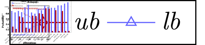
Figure 4: Comparison between the number of states of the concrete and the final abstract model.

Table 1 compares our experimental results of the value iteration for the concrete system and with our abstraction refinement framework. We computed the maximum reachability probability $p_{\mathit{max}}$ for different time bounds. We used precision $\epsilon=0.01$ for the value iteration as well as for the abstraction refinement.

The first column contains the name of the considered model. The blocks titled “Concrete Model” and “Abstraction” present the results for the concrete model and for the final result of the abstraction refinement, respectively. The first two columns denote the name of the instance and the applied time bound $\mathit{tb}$. The third and sixth columns (“#states”) contain the number of states of the concrete model and the final abstraction. Due to the fact that solving a discretised system is rather expensive [29], the benchmark instances are relatively small.

Column “$p$” denotes the computed maximum probability for the concrete system, whereas “$\mathit{lb}$” and “$\mathit{ub}$” denote the computed lower and upper bounds for the abstraction. Column “#iter.” contains the number of iterations of the refinement loop. Column “time” states the computation time needed for the analysis of the concrete model, whereas columns “ref. time” and “val. time” contain the time spent on computing the abstraction refinement and the value iteration. All time measurements are given in the format “minutes:seconds”. The total computation time needed by the prototype is the sum of the time needed for abstraction refinement and the time needed for the value iteration. As can be seen, the time needed for the abstraction refinement is negligible for the most part.

Computations which took longer than five hours were aborted and are marked with “(TO)”. All experiments were done on a Dual Core AMD Opteron processor with 2.4 GHz per core and 64 GB of memory. Each computation needed less than 4 GB memory, we therefore do not present measurements of the memory consumption.

For most instances of PrG and GFS the abstraction refinement needs less computation time than the value iteration for the concrete model. For most instances of PoS both approaches need about the same time. For some instances, e. g. PoS-3-3, the abstraction refinement is slower than the value iteration. For all case studies we were able to achieve a significant compaction of the state space. The latter is also illustrated in Figure 4, which uses a logarithmic scale. If we increase $\epsilon$ and thereby lower the precision, less time is needed for the computation and further compaction is achieved.

Figure 5: Development of $\mathit{lb}$ and $\mathit{ub}$.

Fig 5 shows the development of the probability bounds $\mathit{lb}$ and $\mathit{ub}$ during the abstraction refinement loop for selected instances. The fluctuations which can be seen in the curves for PoS-2-3-conf are due to the increase of accuracy over time.

5 Conclusion

In this paper we have presented our menu-based game abstraction of MA, which is a combination of successful techniques for the abstraction of PA [19, 27]. We also have shown how to analyse the quality of the abstraction for bounded reachability objectives. Should the abstraction turn out to be too coarse, we may refine it using a scheduler-based refinement method which we optimised with a number of additional techniques. Our experiments give promising results and we can report on a significant reduction of the number of states.

As future work we plan to implement a pure game-based abstraction for MA and to compare it to the results of our combined approach. We are also working on the analysis of additional types of properties, e. g. expected time of reachability and long-run average. Furthermore, we are going to explore the possibilities of alternative refinement techniques.

References

- [1]
- [2] Christel Baier, Boudewijn R. Haverkort, Holger Hermanns & Joost-Pieter Katoen (2003): Model-Checking Algorithms for Continuous-Time Markov Chains. IEEE Trans. on Software Engineering 29(6), pp. 524–541, 10.1109/TSE.2003.1205180.
- [3] Hichem Boudali, Pepijn Crouzen & Mariëlle Stoelinga (2010): A Rigorous, Compositional, and Extensible Framework for Dynamic Fault Tree Analysis. IEEE Trans. Dependable Sec. Comput. 7(2), pp. 128–143, 10.1109/TDSC.2009.45.
- [4] Marco Bozzano, Alessandro Cimatti, Joost-Pieter Katoen, Viet Yen Nguyen, Thomas Noll & Marco Roveri (2011): Safety, Dependability and Performance Analysis of Extended AADL Models. Computer Journal 54(5), pp. 754–775, 10.1093/comjnl/bxq024.
- [5] Nicolas Coste, Holger Hermanns, Etienne Lantreibecq & Wendelin Serwe (2009): Towards Performance Prediction of Compositional Models in Industrial GALS Designs. In: Proc. of CAV, LNCS 5643, Springer, pp. 204–218, 10.1007/978-3-642-02658-4_18.
- [6] Pedro R. D’Argenio, Bertrand Jeannet, Henrik E. Jensen & Kim G. Larsen (2002): Reduction and Refinement Strategies for Probabilistic Analysis. In: Proc. of PAPM-PROBMIV, pp. 57–76, 10.1007/3-540-45605-8_5.
- [7] Yuxin Deng & Matthew Hennessy (2013): On the semantics of Markov automata. Information and Computation 222, pp. 139–168, 10.1016/j.ic.2012.10.010.
- [8] Josee Desharnais, Radha Jagadeesan, Vineet Gupta & Prakash Panangaden (2002): The Metric Analogue of Weak Bisimulation for Probabilistic Processes. In: Proc. of LICS, IEEE CS, pp. 413–422, 10.1109/LICS.2002.1029849.
- [9] Christian Eisentraut, Holger Hermanns, Joost-Pieter Katoen & Lijun Zhang (2013): A Semantics for Every GSPN. In: Proc. of Petri Nets, LNCS 7927, Springer, pp. 90–109, 10.1007/978-3-642-38697-8_6.
- [10] Christian Eisentraut, Holger Hermanns & Lijun Zhang (2010): Concurrency and Composition in a Stochastic World. In: Proc. of CONCUR, LNCS 6269, Springer, pp. 21–39, 10.1007/978-3-642-15375-4_3.
- [11] Christian Eisentraut, Holger Hermanns & Lijun Zhang (2010): On Probabilistic Automata in Continuous Time. In: Proc. of LICS, IEEE CS, pp. 342–351, 10.1109/LICS.2010.41.
- [12] Sanjay Ghemawat, Howard Gobioff & Shun-Tak Leung (2003): The Google file system. In: Proc. of the ACM Symp. on Operating Systems Principles (SOSP), ACM Press, pp. 29–43, 10.1145/945445.945450.
- [13] D. Guck (2012): Quantitative Analysis of Markov Automata. Master’s thesis, RWTH Aachen University.
- [14] Dennis Guck, Tingting Han, Joost-Pieter Katoen & Martin R. Neuhäußer (2012): Quantitative Timed Analysis of Interactive Markov Chains. In: Proc. of NFM, LNCS 7226, Springer, pp. 8–23, 10.1007/978-3-642-28891-3_4.
- [15] Dennis Guck, Hassan Hatefi, Holger Hermanns, Joost-Pieter Katoen & Mark Timmer (2013): Modelling, Reduction and Analysis of Markov Automata. In: Proc. of QEST, LNCS 8054, Springer, pp. 55–71, 10.1007/978-3-642-40196-1_5.
- [16] Hassan Hatefi & Holger Hermanns (2012): Model Checking Algorithms for Markov Automata. ECEASST 53, 10.1007/978-3-642-40213-5_16.
- [17] Boudewijn R. Haverkort, Matthias Kuntz, Anne Remke, S. Roolvink & Mariëlle Stoelinga (2010): Evaluating repair strategies for a water-treatment facility using Arcade. In: Proc. of DSN, IEEE, pp. 419–424, 10.1109/DSN.2010.5544290.
- [18] Holger Hermanns (2002): Interactive Markov Chains – The Quest for Quantified Quality. LNCS 2428, Springer, 10.1007/3-540-45804-2.
- [19] Mark Kattenbelt, Marta Z. Kwiatkowska, Gethin Norman & David Parker (2010): A game-based abstraction-refinement framework for Markov decision processes. Formal Methods in System Design 36(3), pp. 246–280, 10.1007/s10703-010-0097-6.
- [20] Marco Ajmone Marsan, Gianni Conte & Gianfranco Balbo (1984): A Class of Generalized Stochastic Petri Nets for the Performance Evaluation of Multiprocessor Systems. ACM Trans. Comput. Syst. 2(2), pp. 93–122, 10.1145/190.191.
- [21] John F. Meyer, Ali Movaghar & William H. Sanders (1985): Stochastic Activity Networks: Structure, Behavior, and Application. In: Proc. of PNPM, IEEE CS, pp. 106–115.
- [22] Martin R. Neuhäußer (2010): Model checking nondeterministic and randomly timed systems. Ph.D. thesis, RWTH Aachen University and University of Twente.
- [23] Roberto Segala (1995): Modeling and Verification of Randomized Distributed Real-Time Systems. Ph.D. thesis, MIT.
- [24] Lloyd S Shapley (1953): Stochastic games. Proceedings of the National Academy of Sciences of the United States of America 39(10), p. 1095, 10.1073/pnas.39.10.1095.
- [25] Mark Timmer, Joost-Pieter Katoen, Jaco van de Pol & Mariëlle Stoelinga (2012): Efficient Modelling and Generation of Markov Automata. In: Proc. of CONCUR, LNCS 7454, Springer, pp. 364–379, 10.1007/978-3-642-32940-1_26.
- [26] Mark Timmer, Jaco van de Pol & Mariëlle Stoelinga (2013): Confluence Reduction for Markov Automata. In: Proc. of FORMATS, LNCS 8053, Springer, pp. 243–257, 10.1007/978-3-642-40229-6_17.
- [27] Björn Wachter (2011): Refined probabilistic abstraction. Ph.D. thesis, Saarland University.
- [28] Björn Wachter & Lijun Zhang (2010): Best Probabilistic Transformers. In: Proc. of VMCAI, LNCS 5944, Springer, pp. 362–379, 10.1007/978-3-642-11319-2_26.
- [29] Lijun Zhang & Martin R. Neuhäußer (2010): Model Checking Interactive Markov Chains. In: Proc. of TACAS, LNCS 6015, Springer, pp. 53–68, 10.1007/978-3-642-12002-2_5.