Pion TMDs in light-front constituent approach, and
Boer-Mulders effect in the pion-induced Drell-Yan process

Abstract

At leading twist the transverse-momentum dependent parton distributions of the pion consist of two functions, the unpolarized $f_{1,\pi}(x,\boldsymbol{k}^{\,2}_{\perp})$ and the Boer-Mulders function $h_{1,\pi}^{\perp}(x,\boldsymbol{k}^{\,2}_{\perp})$. We study both functions within a light-front constituent model of the pion, comparing the results with different pion models and the corresponding nucleon distributions from a light-front constituent model. After evolution from the model scale to the relevant experimental scales, the results for the collinear pion valence parton distribution function $f_{1,\pi}(x)$ are in very good agreement with available parameterizations. Using the light-front constituent model results for the Boer-Mulders functions of the pion and nucleon, we calculate the coefficient $\nu$ in the angular distribution of Drell-Yan dileptons produced in pion-nucleus scattering, which is responsible for the violation of the Lam-Tung relation. We find a good agreement with data, and carefully discuss the range of applicability of our approach.

I Introduction

Transverse momentum dependent distribution functions (TMDs) Collins:1981uw ; Collins:2003fm ; Collins-book provide unique insights in the 3D hadronic structure Tangerman:1994eh ; Kotzinian:1994dv ; Mulders:1995dh ; Boer:1997nt ; Bacchetta:2006tn , by taking into account the transverse motion of partons and spin-orbit correlations. The Drell-Yan process (DY) Christenson:1970um ; Drell:1970wh is basically the only source for this type of information for hadrons other than the nucleon, that are available as secondary beams in high energy experiments, such as the pion which is the main focus of this work. DY experiments with pions were reported in Refs. Badier:1981ti ; Palestini:1985zc ; Falciano:1986wk ; Guanziroli:1987rp ; Conway:1989fs ; Bordalo:1987cs , see Stirling:1993gc for a compilation of DY data till 1993 and McGaughey:1999mq ; Reimer:2007iy ; Arnold:2008kf ; Chang:2013opa ; Peng:2014hta for reviews of later data and theoretical progress. TMDs describe hard processes like DY on the basis of factorization theorems Collins:1981uk ; Ji:2004wu ; Collins:2004nx ; Echevarria:2011rb . The QCD evolution properties of some of the TMDs were studied in Refs. Collins-book and Collins:1984kg ; Aybat:2011zv ; Aybat:2011ge ; Cherednikov:2007tw ; Bacchetta:2013pqa ; Echevarria:2012pw ; Vladimirov:2014aja .

This work is devoted to the study of leading-twist TMDs of the pion. At leading twist the pion structure is described in terms of two TMDs, $f_{1,\pi}(x,\boldsymbol{k}^{2}_{\perp})$ and $h_{1,\pi}^{\perp}(x,\boldsymbol{k}^{2}_{\perp})$. The unpolarized TMD $f_{1,\pi}(x,\boldsymbol{k}^{2}_{\perp})$ describes the distribution of unpolarized partons carrying the longitudinal momentum fraction $x$ of the pion, and the transverse momentum $k_{\perp}$. The so-called Boer-Mulders function $h_{1,\pi}^{\perp}(x,\boldsymbol{k}^{2}_{\perp})$ Boer:1997nt ; Boer:1999mm describes a spin-orbit correlation of transversely polarized partons, which is chiraly and (“naively”) time-reversal odd. “Chiraly odd” means that the operator structure defining $h_{1,\pi}^{\perp}(x,\boldsymbol{k}^{2}_{\perp})$ flips the chirality of the partons, implying that this function can enter the description of a process only in combination with another chiral odd function. “Time reversal odd” (T-odd) means that under time reversal transformations the correlation flips sign, while the Wilson lines inherent in the TMD operator definitions are transformed from future- to past-pointing or vice versa. This implies that T-odd functions appear with different signs in deep-inelastic scattering (DIS) and DY process Brodsky:2002cx ; Collins:2002kn ; Ji:2002aa ; Brodsky:2002rv ; Boer:2002ju ; Belitsky:2002sm ; Boer:2003cm . The different signs of T-odd TMDs in different processes can be tested experimentally in the case of the nucleon, though this is not feasible for the pion.

However, the T-odd correlations as described by the Boer-Mulders functions in pion and nucleon may be responsible for the violation of the Lam-Tung relation, which connects the coefficients in the angular distribution of the DY lepton pairs Lam:1978pu ; Collins:1978yt ; Mirkes:1994dp . The $\pi$-nucleus DY data Falciano:1986wk ; Guanziroli:1987rp ; Conway:1989fs show a significant violation of this relation, which calls for a nonperturbative leading-twist mechanism beyond collinear factorization. The Boer-Mulders effect provides such a mechanism within the TMD factorization framework Boer:1999mm , though alternative mechanisms have also been proposed Brandenburg:1993cj ; Brandenburg:1994wf ; Boer:2004mv ; Brandenburg:2006xu ; Nachtmann:2014qta . Indications for the violation of the Lam-Tung relation were also observed in $pp$- and $pd$-induced DY Zhu:2006gx .

In order to perform the nonperturbative calculations of the pion TMDs $f_{1,\pi}(x,\boldsymbol{k}^{2}_{\perp})$ and $h_{1,\pi}^{\perp}(x,\boldsymbol{k}^{2}_{\perp})$ we use the light-front formalism, where hadrons are described in terms of light-front wave functions (LFWFs). The latter are expressed as an expansion of various quark, antiquark and gluon Fock components. In principle, there is an infinite number of LFWFs in such an expansion. However, there are many situations where one can successfully model hadronic wave functions by confining oneself to the contribution of the minimal Fock-space configuration with a few partons. We will refer to this approach as the light-front constituent model (LFCM). The LFCM was successfully applied to describe many nucleon properties Boffi:2002yy ; Boffi:2003yj ; Pasquini:2004gc ; Pasquini:2005dk ; Pasquini:2006iv ; Pasquini:2007xz ; Pasquini:2007iz ; Boffi:2007yc ; Pasquini:2009ki ; Lorce:2011dv including TMDs Pasquini:2008ax ; Boffi:2009sh ; Pasquini:2010af ; Pasquini:2011tk . For the pion, the specific model we will adopt for the minimal Fock-space components of the LFWF has been originally proposed in Refs. Schlumpf:1994bc ; Chung:1988mu , and has been applied to study some partonic properties of pion in Refs. Frederico:2009fk ; Salme':2012rv . However, the present work is the first application to study the TMDs in the pion.

The description of nucleon TMDs within the LFCM was shown to agree with phenomenology within (10-30)$\,\%$ in the valence-$x$ region after evolution from the low initial scale of the model to experimentally relevant scales Boffi:2009sh ; Pasquini:2011tk . This is in particular the case for the Boer-Mulders function of the nucleon Pasquini:2011tk .

In this work we derive and calculate the unpolarized TMD and Boer-Mulders function of the pion, $f_{1,\pi}(x,\boldsymbol{k}^{2}_{\perp})$ and $h_{1,\pi}^{\perp}(x,\boldsymbol{k}^{2}_{\perp})$, and compute the coefficient $\nu$ in $\pi$-nucleus induced DY. We find that the valence distribution function $f_{1,\pi}(x)$ of the pion obtained from the LFCM agrees well with available parameterizations. We compare our results for the pion Boer-Mulder function with previous results from spectator and bag models Refs. Lu:2004hu ; Burkardt:2007xm ; Gamberg:2009uk ; Lu:2012hh as well as with lattice QCD Engelhardt:2013nba . We show that $h_{1,\pi}^{\perp}(x,\boldsymbol{k}^{2}_{\perp})$, in combination with the nucleon Boer-Mulders function $h_{1,N}^{\perp}(x,\boldsymbol{k}^{2}_{\perp})$ from the LFCM of Ref. Pasquini:2010af , gives a good description of the DY data on the coefficient $\nu$. For other model studies of nucleon Boer-Mulders function and phenomenological work related to the violation of the Lam-Tung relation we refer to Refs. Boer:1999mm and Bianconi:2006hc ; Lu:2005rq ; Gamberg:2005ip ; Sissakian:2005yp ; Barone:2006ws ; Zhang:2008nu ; Lu:2009ip ; Barone:2010gk ; Lu:2011mz ; Liu:2012fha ; Liu:2012vn ; Chang:2013pba ; Chen:2013zpy .

The outline of this work is as follows. In Sec. II we determine the initial scale of the pion LFCM approach. In Sec. III we review the classification of the pion light-front wave function, in the minimal ($q\bar{q}$) Fock space configuration, in terms of light-front amplitudes describing the different $\bar{q}q$ orbital angular momentum components in the pion state. In Sec. IV we derive the representation of the leading-twist pion TMDs as overlap of light-front amplitudes. In Sec. V we use a specific model for the pion LFWFs to obtain numerical results for pion TMDs at the initial hadronic scale. We then evolve and discuss our results. Sec. VI gives a brief review of the DY formalism at a leading-order parton-model level. Sec. VII is dedicated to a discussion of the unpolarized TMD in the DY process, and establishes the range of applicability of our approach. In Sec. VIII we discuss the Boer-Mulders effect in $\pi$-nucleus induced DY. Finally, in Sec. IX we summarize our results and give an outlook.

II Initial scale of pion constituent approach

Parton distribution functions are defined within a certain regularization scheme at a given renormalization scale. The results from a constituent approach refer to an assumed low initial scale $\mu_{0}$, at which a pion is thought to consist of a “valence” quark-antiquark pair only, while a nucleon is similarly assumed to consist of 3 “valence” quarks only. The value of $\mu_{0}$ is not known a priori, but it can be determined in a way independent of the details of the constituent model. Therefore we shall first address this point, before embarking with the actual study of TMDs in LFCM.

It is crucial to determine $\mu_{0}$ for two reasons. First, the model parton distributions have to be evolved from a well-defined initial scale $\mu_{0}$ to experimentally relevant scales $Q\sim$ few GeV before they can be confronted with data. Second, the initial scale $\mu_{0}$ determines the value of the running coupling constant $\alpha_{s}(\mu_{0}^{2})$ which enters the overall normalization of the Boer-Mulders function, when the initial (final) state interaction effects are taken into account via the one-gluon exchange mechanism (see the discussion in in Sec. IV.2).

To determine $\mu_{0}$ we use the following standard procedure Pasquini:2004gc ; Broniowski:2007si ; Davidson:2001cc ; Courtoy:2008nf . At the initial scale the entire pion momentum must be carried by valence $\bar{q}$, $q$ degrees of freedom, $\langle x\rangle_{v}=1$, while sea-quark and gluon contributions are set to zero. Similarly to Ref. Broniowski:2007si we then require the initial scale $\mu_{0}$ to be such that after evolution from $\mu_{0}$ to say $Q^{2}=4\,{\rm GeV}^{2}$ the phenomenological value for the pion momentum fraction carried by valence quarks is reproduced. We take

$$\langle x\rangle_{v} = \int_{0}^{1}{\rm d}x\;x\biggl{[}(f_{1,\pi^{+}}^{u}-f_{1,\pi^{+}}^{\bar{u}})(x)+(f_{1,\pi^{+}}^{\bar{d}}-f_{1,\pi^{+}}^{d})(x)\biggr{]}$$ (1)

$$= 0.47\pm 0.02\;\;\mbox{at $\;Q^{2}=4$ GeV${}^{2}$}$$

in leading (LO) and next-to-leading order (NLO) from the parameterizations Sutton:1991ay ; Gluck:1999xe . We use $\alpha_{\rm LO}(M^{2}_{Z})=0.13939$ and $\alpha_{\rm NLO}(M_{Z}^{2})=0.12018$ in $\overline{\rm MS}$ scheme for the strong coupling constant at the $Z_{0}$ mass $M_{Z}=91.1$ GeV from the global fit of parton distribution functions (PDFs) to hard-scattering data from Ref. Martin:2009iq . These values correspond to $\Lambda_{\rm LO}=359,\,322,\,255$ MeV and $\Lambda_{\rm NLO}=402,\,341,\,239$ MeV for respectively $N_{F}=3,\,4,\,5$ flavors in the variable flavor-number scheme with heavy-quark mass thresholds at $m_{c}=1.4$ GeV, $m_{b}=4.75$ GeV, $m_{t}=175$ GeV Martin:2009iq .

With these parameters the above described procedure yields at LO and NLO for the initial scale

$$\mu_{0,{\rm LO}} = 460\,\mbox{MeV},\;\;\;\;\;\frac{\alpha_{{\rm LO}}(\mu_{0}^{2})}{4\pi}=0.225,$$ (2)

$$\mu_{0,{\rm NLO}} = 555\,\mbox{MeV},\;\;\;\;\;\frac{\alpha_{{\rm NLO}}(\mu_{0}^{2})}{4\pi}=0.0938.$$ (3)

In a different NLO scheme the numerical values in Eq. (3) would be somewhat different, but it is beyond the scope of this work to study scheme-dependence effects. In the following we shall assume that theoretical uncertainties due to scheme dependence are smaller than the generic accuracy of (light-front) constituent model approaches.

At this point it is instructive to compare the LO and NLO initial scales for pion distribution functions, Eqs. (2)-(3), with those obtained in the case of the nucleon Pasquini:2011tk . In principle, the constituent model approaches for pion and nucleon can be viewed as unrelated models. Nevertheless, the underlying physical assumption is the same. At some low “hadronic scale” one deals with constituent (“valence”) degrees of freedom carrying the total hadron momentum: a constituent quark-antiquark pair in the pion case, or 3 constituent quarks in the nucleon case. For the underlying physical picture to be successful one should expect the initial scale to be “universal,” i.e. independent of the considered hadron. It is therefore gratifying to observe how close numerically the results are for the nucleon case (in Pasquini:2011tk it was obtained $\mu_{0,\rm LO}=420\,\mbox{MeV}$ and $\mu_{0,{\rm NLO}}=508\,\mbox{MeV}$ for the nucleon) as compared to the pion case in Eqs. (2)-(3). This is an encouraging indication for the usefulness of the constituent model picture.

III Light-front amplitudes in pion constituent approach

In this section, we review the classification of the light-front wave function for the pion, considering the minimal Fock space configuration, i.e. $q\bar{q}$. According to the total quark orbital angular momentum projection, the $q\bar{q}$ LFWF of the pion can be written in terms of two light-front amplitudes carrying the total quark orbital angular momentum $l_{z}=0$ and $|l_{z}=1|$, i.e.

$$|\pi(p)\rangle_{q\bar{q}}=|\pi(p)\rangle_{q\bar{q}}^{l_{z}=0}+|\pi(p)\rangle_{q\bar{q}}^{|l_{z}=1|}.$$ (4)

The different angular-momentum components of the state in Eq. (4) are given by Burkardt:2002uc ; Ji:2003yj

$$|\pi(p)\rangle_{q\bar{q}}^{l_{z}=0} = T_{\pi}\,\int d[1]d[2]\psi^{(1)}(1,2)\frac{\delta_{ij}}{\sqrt{3}}\left[q^{\dagger}_{i\uparrow}(1)\bar{q}^{\dagger}_{j\downarrow}(2)-q^{\dagger}_{i\downarrow}(1)\bar{q}^{\dagger}_{j\uparrow}(2)\right]|0\rangle\ ,$$ (5)

$$|\pi(p)\rangle_{q\bar{q}}^{|l_{z}|=1} = T_{\pi}\,\int d[1]d[2]\psi^{(2)}(1,2)\frac{\delta_{ij}}{\sqrt{3}}\left[k_{1\perp}^{-}q^{\dagger}_{i\uparrow}(1)\bar{q}^{\dagger}_{j\uparrow}(2)+k_{1\perp}^{+}q^{\dagger}_{i\downarrow}(1)\bar{q}^{\dagger}_{j\downarrow}(2)\right]|0\rangle\ ,$$ (6)

where $k^{\pm}_{i\perp}=k^{x}_{i}\pm k^{y}_{i}$, and $q^{\dagger}_{i\lambda}$ and $\bar{q}^{\dagger}_{i\lambda}$ are creation operators of a quark and antiquark with flavor $q$, helicity $\lambda$ and color $i$, respectively. In Eqs. (5) and (6), $T_{\pi}$ is the isospin factor which projects on the different members of the isotriplet of the pion, and is defined as $T_{\pi}=\sum_{\tau_{q}\tau_{\bar{q}}}\langle 1/2\tau_{q}1/2\tau_{\bar{q}}|1\tau_{\pi}\rangle$ with $\tau_{q},\tau_{\bar{q}}$ and $\tau_{\pi}$ the isospin of the quark, antiquark and pion state, respectively. Furthermore, the amplitudes $\psi^{(1,2)}(1,2)$ are functions of quark momenta with arguments 1 representing $x_{1}$ and $\boldsymbol{k}_{1\perp}$ and so on. They depend on the transverse momenta only through scalar products, e.g. $\boldsymbol{k}_{i\perp}\cdot\boldsymbol{k}_{j\perp}$. Since momentum conservation implies $\boldsymbol{k}_{1\perp}+\boldsymbol{k}_{2\perp}=0$ and $x_{1}+x_{2}=1$, $\psi^{(1,2)}_{q\bar{q}}(1,2)$ depend only on the variables $\bar{x}=x_{1}$ and $\boldsymbol{\kappa}_{\perp}^{2}$, with $\boldsymbol{\kappa}_{\perp}=\boldsymbol{k}_{1\perp}$. The integration measure in Eqs. (5) and (6) is defined as

$$d[1]d[2]=\frac{dx_{1}dx_{2}}{\sqrt{x_{1}x_{2}}}\delta\left(1-\sum_{i=1}^{2}x_{i}\right)\frac{d^{2}\boldsymbol{k}_{1\perp}d^{2}\boldsymbol{k}_{2\perp}}{[2(2\pi^{3})]}\delta^{2}\left(\sum_{i=1}^{2}\boldsymbol{k}_{i\perp}\right)=\frac{d\bar{x}}{\sqrt{\bar{x}(1-\bar{x})}}\frac{d^{2}\boldsymbol{\kappa}_{\perp}}{[2(2\pi^{3})]}.$$ (7)

In the following, we will describe the above LFWF amplitudes in a light-front constituent model which was already successfully applied for describing the charge form factor and decay constant of the pion Chung:1988mu ; Schlumpf:1994bc and the generalized parton distributions Frederico:2009fk ; Salme':2012rv .

The $q\bar{q}$ component of the light-front state of the pion can be written as

$$\hbox{$|\pi(p)\rangle$}_{q\bar{q}}=T_{\pi}\,\sum_{\lambda_{i},c_{i}}\int d[1]d[2]\Psi^{[f]}_{q\bar{q}}(\{x_{i},\boldsymbol{k}_{i\perp};\lambda_{i}\})\frac{\delta_{ij}}{\sqrt{3}}q^{\dagger}_{i\lambda_{1}}(1)\bar{q}^{\dagger}_{j\lambda_{2}}(2)|0\rangle\,.$$ (8)

In Eq. (8), the LFWF $\Psi^{[f]}_{q\bar{q}}(\{x_{i},\boldsymbol{k}_{i\perp};\lambda_{i}\})$ satisfies Poincarè covariance and is an eigenstate of the total angular momentum operator in the light-front dynamics. These properties can be fulfilled by constructing the wave function as the product of a momentum wave function, which is spherically symmetric and invariant under permutation of the two constituent partons, and a spin wave function, which is uniquely determined by symmetry requirements, i.e.,

$$\Psi^{[f]}_{q\bar{q}}(\{x_{i},\boldsymbol{k}_{i\perp};\lambda_{i}\}) = \tilde{\psi}_{\pi}(\bar{x},\boldsymbol{\kappa}_{\perp})\tilde{\Phi}(\lambda_{1},\lambda_{2}).$$ (9)

In the above equation, the spin-dependent part is given by

$$\tilde{\Phi}(\lambda_{1},\lambda_{2}) = \sum_{\mu_{1}\mu_{2}}\langle 1/2,\mu_{1};1/2,\mu_{2}|0,0\rangle D_{\mu_{1}\lambda_{1}}^{1/2*}(R_{M}(\boldsymbol{\kappa}))D_{\mu_{2}\lambda_{2}}^{1/2*}(R_{M}(-\boldsymbol{\kappa})),$$ (10)

where $\boldsymbol{\kappa}=\{\boldsymbol{\kappa}_{\perp},\kappa_{z}\}$, with

$$\kappa_{z}=M_{0}(\bar{x},\boldsymbol{\kappa}_{\perp})(\bar{x}-\frac{1}{2}),$$ (11)

and the free mass defined as

$$M_{0}^{2}(\bar{x},\boldsymbol{\kappa}_{\perp})=\frac{m^{2}+|\boldsymbol{\kappa}_{\perp}|^{2}}{\bar{x}(1-\bar{x})},$$ (12)

with $m$ the quark mass. In Eq. (10), $D_{\lambda\mu}^{1/2}(R_{M}(\bar{x},\boldsymbol{\kappa}_{\perp}))$ is the matrix element of the Melosh rotation $R_{M}$ Melosh:1974cu

$$D_{\lambda\mu}^{1/2}(R_{M}(\boldsymbol{\kappa})) = \langle\lambda|R_{M}(\boldsymbol{\kappa})|\mu\rangle$$ (13)

$$= \langle\lambda|\frac{m+\bar{x}M_{0}-i\boldsymbol{\sigma}\cdot(\hat{\boldsymbol{z}}\times\boldsymbol{\kappa}_{\perp})}{\sqrt{(m+\bar{x}M_{0})^{2}+\boldsymbol{\kappa}^{\,2}_{\perp}}}|\mu\rangle.$$

The Melosh rotation corresponds to the unitary transformation which converts the Pauli spinors of the quark and antiquark in the pion rest-frame to the light-front spinor. Making explicit the dependence on the quark and antiquark helicities, the spin wave function of Eq. (10) takes the following values:

$$\tilde{\Phi}\left(\uparrow,\uparrow\right) = \prod_{i}\frac{1}{\sqrt{N(x_{i},\boldsymbol{\kappa}_{\perp})}}\kappa_{\perp}^{-}(-a_{1}+a_{2}),$$ (14)

$$\tilde{\Phi}\left(\uparrow,\downarrow\right) = \prod_{i}\frac{1}{\sqrt{N(x_{i},\boldsymbol{\kappa}_{\perp})}}(a_{1}a_{2}-\kappa_{\perp}^{+}\kappa^{-}_{\perp}),$$ (15)

$$\tilde{\Phi}\left(\downarrow,\uparrow\right) = \prod_{i}\frac{1}{\sqrt{N(x_{i},\boldsymbol{\kappa}_{\perp})}}(-a_{1}a_{2}+\kappa_{\perp}^{+}\kappa^{-}_{\perp}),$$ (16)

$$\tilde{\Phi}_{\uparrow}\left(\downarrow,\downarrow\right) = \prod_{i}\frac{1}{\sqrt{N(x_{i},\boldsymbol{\kappa}_{\perp})}}\kappa_{\perp}^{+}(-a_{1}-a_{2}),$$ (17)

where $a_{i}=(m+x_{i}M_{0})$, and $N(x_{i},\boldsymbol{\kappa}_{\perp})=[(m+x_{i}M_{0})^{2}+\boldsymbol{\kappa}^{2}_{\perp}]$. Taking into account the quark-helicity dependence in Eqs. (14)-(17), the pion state can be mapped out into the different angular momentum components. As a result, the pion wave function amplitudes in the light-front CQM read

$$\psi^{(1)}(1,2) = \tilde{\psi}(x,\boldsymbol{\kappa}_{\perp})\prod_{i}\frac{1}{\sqrt{N(x_{i},\boldsymbol{\kappa}_{\perp})}}\frac{1}{\sqrt{2}}(a_{1}a_{2}-\kappa_{\perp}^{-}\kappa_{\perp}^{+}),$$ (18)

$$\psi^{(2)}(1,2) = \tilde{\psi}(x,\boldsymbol{\kappa}_{\perp})\prod_{i}\frac{1}{\sqrt{N(x_{i},\boldsymbol{\kappa}_{\perp})}}\frac{1}{\sqrt{2}}(-a_{1}-a_{2}).$$ (19)

IV Twist-2 TMDs in pion constituent approach

The quark TMDs are defined through the following correlation function Mulders:1995dh ; Boer:1997nt ; Bacchetta:2006tn

$$\Phi_{ij}(x,\boldsymbol{k}_{\perp}^{2})=\int\frac{d\xi^{-}d^{2}\boldsymbol{\xi}_{\perp}}{(2\pi)^{3}}e^{i\xi\cdot k}\langle p|\bar{\psi}_{j}(0){\cal L}^{\dagger}(0,\boldsymbol{0}_{\perp}|n){\cal L}(\xi^{-},\boldsymbol{\xi}_{\perp}|n)\psi_{i}(\xi)|p\rangle|_{\boldsymbol{\xi}^{+}=0}\ ,$$ (20)

where $x=k^{+}/p^{+}$ and for a generic four-vector $a^{\mu}=(a^{+},a^{-},\boldsymbol{a}_{\perp})$ we used the light-front components $a^{\pm}=(a^{0}\pm a^{3})/\sqrt{2}$. The Wilson lines ${\cal L}$ connecting the two quarks fields ensure the color gauge invariance of the correlator in Eq. (20) and are defined as Mulders:1995dh ; Boer:1997nt ; Bacchetta:2006tn

$${\cal L}(\xi^{-},{\boldsymbol{\xi}}_{\perp}|n)={\cal P}\exp\left(-ig\int_{\boldsymbol{\xi}^{-}}^{n\cdot\infty}{\rm d}\eta^{-}\cdot A^{+}(\eta^{-},\boldsymbol{\xi}_{\perp})\right){\cal P}\exp\left(-ig\int_{\boldsymbol{\xi}_{\perp}}^{\infty}{\rm d}^{2}\boldsymbol{\eta}_{\perp}\cdot\boldsymbol{A}_{\perp}(\xi^{-}=n\cdot\infty,\boldsymbol{\eta}_{\perp})\right)\ ,$$ (21)

where the vector $n$ depends on the process under consideration. For instance, the future-pointing Wilson lines with $n=(0,+1,0)$ are appropriate for defining TMDs in semi-inclusive DIS, whereas in the Drell-Yan process the Wilson line are necessarily past-pointing with $n=(0,-1,0).$ In particular, this reverses the sign of all T-odd distributions functions entering the correlator.

For a pion target, the information content of the correlator (20) is summarized at leading twist by two TMDs that can be projected out from the correlator as follows

$$\frac{1}{2}{\rm Tr}[\Phi\gamma^{+}] = f_{1,\pi}(x,\boldsymbol{k}_{\perp}^{2}),$$ (22)

$$\frac{1}{2}{\rm Tr}[\Phi i\sigma^{i+}\gamma_{5}] = \frac{\varepsilon^{ij}k_{\perp}^{j}}{M_{\pi}}h_{1,\pi}^{\perp}(x,\boldsymbol{k}_{\perp}^{2}).$$ (23)

The function $f_{1,\pi}(x,\boldsymbol{k}^{2}_{\perp})$ is the unpolarized quark distribution, which integrated over $\boldsymbol{k}_{\perp}$ gives the familiar light-front momentum distribution $f_{1,\pi}(x)$ (in the parton model; in the TMD factorization framework the relation is more subtle Collins-book ), and $h_{1,\pi}^{\perp}(x,\boldsymbol{k}^{2}_{\perp})$ is the Boer-Mulders TMD Boer:1997nt , which is a T-odd function, i.e. it changes sign under ”naive time reversal”, defined as usual time reversal, but without interchange of initial and final states. In the following, we will present the model calculation of the Boer-Mulders function for the SIDIS process, denoted as $h_{1,\pi}^{\perp}(x,\boldsymbol{k}^{2}_{\perp})_{{\rm DIS}}$, while for the Boer-Mulders function in the Drell-Yan process we will use $h_{1\,\pi}^{\perp}(x,\boldsymbol{k}^{2}_{\perp})_{{\rm DY}}=-h_{1,\pi}^{\perp}(x,\boldsymbol{k}^{2}_{\perp})_{{\rm DIS}}$ .

IV.1 Unpolarized parton distribution function in the pion

From the definition (22), the $f_{1,\pi}$ TMD to leading order in the gauge field is given by

$$f_{1,\pi}(x,\boldsymbol{k}^{\,2}_{\perp})=\int\frac{d\xi^{-}d^{2}\boldsymbol{\xi}_{\perp}}{(2\pi)^{3}}e^{i(\xi^{-}k^{+}-\boldsymbol{\xi}_{\perp}\cdot\boldsymbol{k}_{\perp})}\langle\pi(p)|\bar{\psi}(0)\gamma^{+}\psi(\xi^{-},\boldsymbol{\xi}_{\perp})|\pi(p)\rangle\ .$$ (24)

By using the canonical expansion of the quark fields in terms of Fock operators and taking into account the $q\bar{q}$ component of the light-front state of the pion in Eq. (8), we find the final result

$$f_{1,\pi}^{q}(x,\boldsymbol{k}^{2}_{\perp})=f_{1,\pi}^{\bar{q}}(x,\boldsymbol{k}^{2}_{\perp}) = T^{2}_{\pi}\int d[1]d[2]\sqrt{x_{1}x_{2}}\delta(x-x_{1})\delta^{2}(\boldsymbol{k}_{\perp}-\boldsymbol{k}_{1\perp})|\tilde{\psi}_{\pi}(x_{1},\boldsymbol{k}_{\perp 1})|^{2}$$ (25)

$$= T^{2}_{\pi}\frac{1}{2(2\pi)^{3}}|\tilde{\psi}_{\pi}(x,\boldsymbol{k}_{\perp})|^{2}.$$

The unpolarized TMD involves a matrix element which is diagonal in the quark orbital angular momentum. As a consequence, it takes the following expression in terms of the wave function amplitudes in Eqs. (5)-(6)

$$f_{1,\pi}^{q}(x,\boldsymbol{k}^{2}_{\perp})=T^{2}_{\pi}\frac{1}{2(2\pi)^{3}}\,2\left[|\tilde{\psi}^{(1)}(x,\boldsymbol{k}_{\perp}^{2})|^{2}+\boldsymbol{k}_{\perp}^{2}|\tilde{\psi}^{(2)}(x,\boldsymbol{k}_{\perp}^{2})|^{2}\right].$$ (26)

IV.2 Boer-Mulders function of the pion

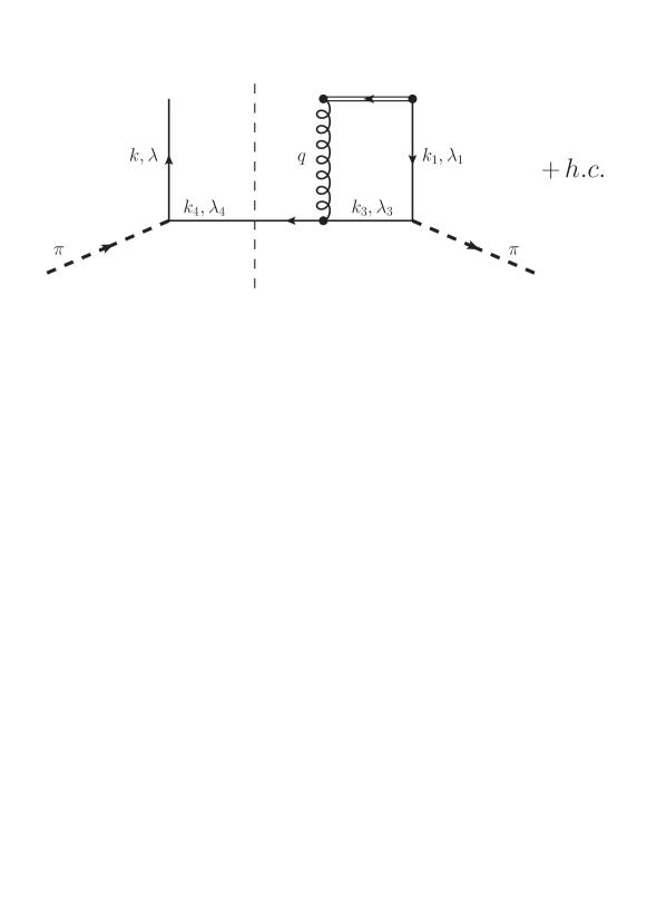
Figure 1: The leading contribution from the one-gluon exchange mechanism to the T-odd distribution function of the pion.

Using the definitions (20) and (23), the quark Boer-Mulders function of the pion is given by

$$h_{1,\pi}^{\perp}(x,\boldsymbol{k}^{\,2}_{\perp})_{{\rm DIS}}=\epsilon^{ij}k^{j}\frac{M_{\pi}}{2\boldsymbol{k}^{\,2}_{\perp}}\int\frac{d\xi^{-}d^{2}\boldsymbol{\xi}_{\perp}}{(2\pi)^{3}}e^{i(\xi^{-}k^{+}-\boldsymbol{\xi}_{\perp}\cdot\boldsymbol{k}_{\perp})}\langle\pi(p)|\bar{\psi}(0){\cal L}^{\dagger}(0,\boldsymbol{0}_{\perp}|\,n)i\sigma^{i+}\gamma_{5}{\cal L}(\xi^{-},\boldsymbol{\xi}_{\perp}|\,n)\psi(\xi^{-},\boldsymbol{\xi}_{\perp})|\pi(p)\rangle\ ,$$ (27)

with $n=(0,+1,0)$. The gauge link ${\cal L}$ is crucial to obtain a non-zero Boer-Mulders function. In the light-front gauge, it reduces to a transverse gauge-link at $\xi^{-}=\infty$, given by the second term in Eq. (21). Furthermore, we expand the above gauge link to take into account the first order non-vanishing contribution corresponding to the one-gluon exchange diagram shown in Fig. 1. Following the procedure outlined in Ref. Pasquini:2010af for the analogous calculation of the T-odd TMDs of the nucleon, we obtain the following result for the quark Boer-Mulders function of the pion

$$h_{1,\pi}^{\perp\,q}(x,\boldsymbol{k}^{\,2}_{\perp})_{{\rm DIS}}=-g^{2}\,M_{\pi}\frac{k^{x}_{\perp}-ik^{y}_{\perp}}{\boldsymbol{k}^{\,2}_{\perp}}\frac{1}{(2\pi)^{11}}\frac{1}{\sqrt{2k^{+}}}\int\frac{{\rm d}k_{3}^{+}{\rm d}^{2}\boldsymbol{k}_{3\perp}}{\sqrt{(2k_{3}^{+})(2k^{+}_{4})}}\int\frac{{\rm d}^{2}\boldsymbol{q}_{\perp}}{2k^{+}_{1}}$$

$$\times\Big{\{}\frac{1}{\boldsymbol{q}^{\,2}_{\perp}}\sum_{\lambda_{3}}\sum_{\bar{q}}\sum_{i.j}\sum_{k,l}T^{a}_{ij}T^{b}_{kl}\delta_{ab}\langle\pi(p)|q^{\dagger}_{i\uparrow}(k_{1})q_{j\downarrow}(k)\bar{q}_{k\lambda_{3}}(k_{4})\bar{q}^{\dagger}_{l\lambda_{3}}(k_{3})|\pi(p)\rangle\Big{\}},$$ (28)

where the parton momenta are defined as $k_{1}=k-q$, $k_{4}=k_{3}-q$. The above equation corresponds to the diagram of Fig. 1 with $\lambda=-\lambda_{1}$ and $\lambda_{4}=\lambda_{3}$ for the helicity of the interacting and spectator partons, respectively, i.e. the helicity is conserved at the antiquark-gluon vertex, while the helicity of the struck quark flips from the initial to the final state. For angular momentum conservation, the quark helicity flip must be compensated by a transfer of one unit of orbital angular momentum. Inserting in Eq. (28) the light-front wave function amplitude decomposition of the pion state introduced in Sec. III, one finds the following results in terms of the light-front amplitudes $\psi^{(i)}$

$$h_{1,\pi}^{\perp\,q}(x,\boldsymbol{k}^{\,2}_{\perp})_{{\rm DIS}} = \frac{4}{3}g^{2}\,T^{2}_{\pi}\,M_{\pi}\frac{k^{x}_{\perp}-ik^{y}_{\perp}}{\boldsymbol{k}^{\,2}_{\perp}}\int\frac{{\rm d^{2}}\boldsymbol{q}_{\perp}}{(2\pi)^{5}}\frac{1}{\boldsymbol{q}^{\,2}_{\perp}}\,{\cal H}_{\pi}^{\perp\,q},$$ (29)

where the function ${\cal H}^{\perp\,q}_{\pi}$ is

$${\cal H}_{\pi}^{\perp\,q} = -k^{\prime+}_{\perp}\psi^{(1)}(1,2)\psi^{(2)*}(1^{\prime},2^{\prime})+k^{+}_{\perp}\psi^{(1)*}(1,2)\psi^{(2)}(1^{\prime},2^{\prime})$$ (30)

with $\boldsymbol{k}^{\prime}_{\perp}=\boldsymbol{k}_{\perp}-\boldsymbol{q}_{\perp}$ and the parton coordinates $1=(x,\boldsymbol{k}_{\perp})$, $2=(1-x,-\boldsymbol{k}_{\perp})$, and $1^{\prime}=(x,\boldsymbol{k}^{\prime}_{\perp})$, $2^{\prime}=(1-x,-\boldsymbol{k}^{\prime}_{\perp})$. In the model for the light-front amplitudes introduced in Sec. III, we find the following explicit results

$$h_{1,\pi}^{\perp\,q}(x,\boldsymbol{k}^{\,2}_{\perp})_{{\rm DIS}}=\frac{4}{3}g^{2}\,T^{2}_{\pi}\,M_{\pi}\frac{k^{x}_{\perp}-ik^{y}_{\perp}}{\boldsymbol{k}^{\,2}_{\perp}}\int\frac{{\rm d}^{2}\boldsymbol{q}_{\perp}}{(2\pi)^{5}}\frac{1}{\boldsymbol{q}^{\,2}_{\perp}}\tilde{\psi}^{*}(\{x^{\prime}_{i}\},\{\boldsymbol{k}^{\prime}_{i\perp}\})\,\tilde{\psi}(\{x_{i}\},\{\boldsymbol{k}_{i\perp}\})$$

$$\times\frac{1}{2}\prod_{i=1}^{2}N^{-1}(\boldsymbol{k}\,^{\prime}_{i})N^{-1}(\boldsymbol{k}_{i})\left[\tilde{A}_{1}A_{2}+\boldsymbol{\tilde{B_{1}}}\cdot\boldsymbol{B}_{2}\right],$$ (31)

where we introduced the definitions

$$\tilde{A}_{1} = (m+x_{1}M_{0})(k^{\prime x}_{1}+ik^{\prime y}_{1})-(m+x^{\prime}_{1}M^{\prime}_{0})(k^{x}_{1}+ik^{y}_{1}),$$

$$\tilde{B}_{1}^{x} = -i(m+x^{\prime}_{1}M^{\prime}_{0})(m+x_{1}M_{0})+i(k^{\prime x}_{1}+ik^{\prime y}_{1})(k^{x}_{1}+ik^{y}_{1}),$$

$$\tilde{B}_{1}^{y} = (m+x^{\prime}_{1}M^{\prime}_{0})(m+x_{1}M_{0})+(k^{\prime}_{1,x}+ik^{\prime}_{1y})(k_{1}^{x}+ik_{1}^{y}),$$

$$\tilde{B}_{1}^{z} = i(m+x^{\prime}_{1}M^{\prime}_{0})(k_{1}^{x}+ik_{1}^{y})+i(m+x_{1}M_{0})(k^{\prime x}_{1}+ik^{\prime y}_{1}),$$ (32)

for the spin-dependent contribution from the active quark, and

$$A_{2} = (m+x_{2}M_{0})(m+x^{\prime}_{2}M^{\prime}_{0})+k^{x}_{2}k^{\prime x}_{2}+k^{y}_{2}k^{\prime y}_{2},$$

$$B_{2}^{x} = -(m+x^{\prime}_{2}M^{\prime}_{0})k^{x}_{2}+(m+x_{2}M_{0})k^{\prime y}_{2},$$

$$B_{2}^{y} = (m+x^{\prime}_{2}M^{\prime}_{0})k^{x}_{2}-(m+x_{2}M_{0})k^{\prime x}_{2},$$

$$B_{2}^{z} = k^{\prime x}_{2}k_{2}^{y}-k^{\prime y}_{2}k^{x}_{2},$$ (33)

for the spin-dependent contribution of the spectator antiquark.

The Boer-Mulders function for the valence antiquark can be obtained through a similar calculation by replacing the antiquark spectator with the quark spectator. As a result, one finds $h_{1,\pi}^{\perp\,\bar{q}}=h_{1,\pi}^{\perp\,q}$.

V Results from a light-front constituent model

Up to this point we made only general assumptions. We have chosen to work in a constituent approach of the pion, and determined its initial scale in Sec. II. We have then chosen to use the light-front formalism and presented in Sec. III a general discussion of light-front amplitudes in the pion constituent approach. In Sec. IV we derived a a model independent representation of the leading-twist pion TMDs as overlap of light-front amplitudes for the $q\bar{q}$ Fock-state of the pion. In this Section we will apply the formalism from Secs. III and IV to obtain predictions for pion TMDs using a specific model for the momentum-dependent part of the light-front wave function.

V.1 Model for the momentum-dependent wave function

The formalism described in the previous sections is applied to a specific choice for the LFCM, namely the model proposed in Refs. Schlumpf:1994bc ; Chung:1988mu . The model is specified by adopting the following exponential form for the momentum-dependent part of the pion wave function

$$\tilde{\psi}_{\pi}(\bar{x},{\boldsymbol{\kappa}}_{\perp})=[2(2\pi)^{3}]^{1/2}\left(\frac{M_{0}(\bar{x},{\boldsymbol{\kappa}}_{\perp})}{4~{}\bar{x}(1-\bar{x})}\right)^{1/2}\frac{1}{\pi^{3/4}\beta^{3/2}}\exp{(-\boldsymbol{\kappa}^{2}/(2\beta^{2}))}.$$ (34)

The wave function in Eq. (34) is normalized as

$$\int_{0}^{1}~{}d\bar{x}\int\frac{d{\boldsymbol{\kappa}}_{\perp}}{2(2\pi)^{3}}~{}|\tilde{\psi}_{\pi}(\bar{x},{\boldsymbol{\kappa}}_{\perp})|^{2}=1$$

(recalling that $d\kappa_{z}=d\bar{x}~{}M_{0}(\bar{x},{\boldsymbol{\kappa}}_{\perp})/[4\bar{x}(1-\bar{x})]$), and depends on the free parameter $\beta$ and the quark mass $m$, which have been fitted to the pion charge radius and decay constant. In particular, we take $m=0.250$ GeV and $\beta=0.3194$ Schlumpf:1994bc . As we are considering only the leading $q\bar{q}$ Fock-space component in the pion LFWF, the quark (antiquark) contribution to the pion distribution functions at the hadronic scale of the model coincides with the valence quark $q_{v}$ (antiquark $\bar{q}_{v}$) contribution, while the sea quark contribution is vanishing. Furthermore, isospin symmetry imposes $j_{\pi^{+}}^{u_{v}}=j_{\pi^{+}}^{\bar{d}_{v}}=j_{\pi^{-}}^{d_{v}}=j_{\pi^{-}}^{\bar{u}_{v}}=\tfrac{1}{2}\,j_{\pi^{0}}^{u_{v}}=\tfrac{1}{2}\,j_{\pi^{0}}^{\bar{u}_{v}}=\tfrac{1}{2}\,j_{\pi^{0}}^{d_{v}}=\tfrac{1}{2}\,j_{\pi^{0}}^{\bar{d}_{v}}$, with $j=f_{1},\,h^{\perp}_{1}$. In the following, we will refer to distributions of valence quarks and antiquarks in charged pions, using the notation $j^{q_{v}}_{\pi}$ and $j^{\bar{q}_{v}}_{\pi}$, respectively.

V.2 Results for $f^{q_{v}}_{1,\pi}(x,\boldsymbol{k}^{2}_{\perp})$ at the hadronic scale

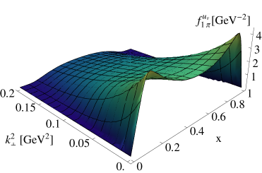
(a)	(b)	(c)

Figure 2: The valence-quark unpolarized TMD of the pion from the LFWF (34) at the hadronic scale. (a) $f_{1,\pi^{+}}^{u_{v}}(x,\boldsymbol{k}_{\perp}^{2})$ as function of $x$ and $\boldsymbol{k}^{2}_{\perp}$. (b) $f_{1,\pi}^{u_{v}}$ as function of $\boldsymbol{k}^{2}_{\perp}$ for selected values of $x$ ($x=0.1$ solid curve, $x=0.3$ dotted curve, $x=0.5$ dashed curve). (c) Comparison of the unpolarized PDFs as functions of $x$ in pion and nucleon from LFCM approaches at their initial hadronic scales. Solid line: $f_{1,\pi}^{u_{v}}(x)$ in the pion, obtained in this work. Dotted (dashed) curve: $f_{1p}^{u_{v}}(x)$ ($f_{1p}^{d_{v}}(x)$) in the proton from the light-front constituent quark model of Ref. Pasquini:2008ax .

In Fig. 2, we show the model predictions for the valence-quark contribution to the unpolarized TMD as function of $x$ and $\boldsymbol{k}^{2}_{\perp}$. The results refer to the low hadronic scale determined in Sec II. For the $q\bar{q}$ component of the pion state, the distribution of quark with longitudinal momentum fraction $x$ is equal to the distribution of antiquark with longitudinal momentum fraction $1-x$, i.e. $f_{1,\pi}^{q_{v}}(x,\boldsymbol{k}^{2}_{\perp})=f_{1,\pi}^{\bar{q}_{v}}(1-x,\boldsymbol{k}^{2}_{\perp})$. Furthermore, one has the relation $f_{1,\pi}^{q_{v}}(x,\boldsymbol{k}^{2}_{\perp})=f_{1,\pi}^{\bar{q}_{v}}(x,\boldsymbol{k}^{2}_{\perp})$, which gives as final result a momentum distribution symmetric with respect to $x=1/2$. We also observe a rapid fall off with $\boldsymbol{k}^{2}_{\perp}$, with a decreasing slope at larger $x$. This behavior can be better seen in Fig. 2b where we plot the $f_{1,\pi}^{u_{v}}$ TMD as function of $\boldsymbol{k}^{2}_{\perp}$ at different values of $x$. We notice that the $\boldsymbol{k}^{2}_{\perp}$ dependence is definitely not Gaussian, but it can be approximated by a Gaussian function with reasonable accuracy. Upon integration over $\boldsymbol{k}_{\perp}$, we obtain the unpolarized PDF. In Fig. 2c we compare the unpolarized quark distribution of the pion $f_{1,\pi}(x)$ with the results of the unpolarized quark distribution of the proton $f_{1,p}(x)$ obtained from the three-quark LFWF of Ref. Pasquini:2008ax . The shape of the distributions for the pion and proton is quite different, reflecting the different valence-quark structure of the hadrons. For the proton, the momentum distribution of the valence-quark is peaked at $x\approx 1/3$. Moreover, the SU(6) symmetry for the spin-flavor structure of the LFWF in Pasquini:2008ax gives $f_{1,p}^{u_{v}}(x)=2f_{1,p}^{d_{v}}(x)$.

V.3 Evolved results for $f^{q_{v}}_{1,\pi}(x)$ in comparison to parametrizations

As a first test of the applicability of the LFCM to the description of partonic properties of the pion, we compare the results for $f_{1,\pi}^{u_{v}}(x)$, evolved from the initial scale of the model to $Q^{2}=25\,{\rm GeV}^{2}$, with available parameterizations  Gluck:1999xe ; Sutton:1991ay ; Owens:1984zj ; Gluck:1991ey ; Hecht:2000xa ; Aicher:2010cb ; Wijesooriya:2005ir (for a review of the pion PDF in the valence-$x$ region see also Ref. Holt:2010vj ). The initial-scale, LO-evolved and NLO-evolved distributions are shown in Fig. 3a. The LO and NLO evolutions are applied starting from the initial scales $\mu_{0,{\rm LO}}^{2}$ and $\mu_{0,{\rm NLO}}^{2}$ in Eqs. (2) and (3), respectively. Remarkably, although the initial scales and especially the values of $\alpha_{s}(\mu_{0}^{2})$ at LO and NLO differ, the evolved results are numerically close. This kind of behavior has been interpreted in Refs. Gluck:1991ey ; Gluck:1999xe ; Gluck:1998xa ; Traini:1997jz as an indication for the “convergence” of perturbation theory down to low scales.

It is important to keep in mind that the LO and NLO parameterizations of Gluck:1991ey ; Gluck:1999xe ; Gluck:1998xa differ slightly at their respective low scales, such that they allow one to describe data equally well in the combination with the LO or NLO hard parts in the respective LO or NLO treatments. In contrast, our model input at the initial scale is identical in LO and NLO. This inevitably introduces a scheme dependence, when applying the model results beyond LO. But we feel that such scheme-dependence effects are smaller than the generic model accuracy, as discussed in Sec. II. Considering that in the context of parton structure studies the generic model accuracy is observed to be around (10–30)$\,\%$ Boffi:2009sh , we interpret the result in Fig. 3a, i.e. the “convergence of the LO and NLO results in the sense of Refs. Gluck:1991ey ; Gluck:1999xe ; Gluck:1998xa ; Traini:1997jz , as an indication that the issue of applicability of perturbative evolution equations down to the low scales in Eqs. (2)-(3) is not the dominant source of theoretical uncertainty in our approach.

(a)	(b)	(c)

Figure 3: (a) $xf_{1,\pi}^{u_{v}}(x)$ as function of $x$. Solid line: at initial scale of the model. Dotted line: LO-evolved to $25\,{\rm GeV}^{2}$. Dashed line: NLO-evolved to $25\,{\rm GeV}^{2}$. (b) $xf_{1,\pi}^{u_{v}}(x)$ as function of $x$ after LO-evolution to $Q^{2}=25$ GeV² in comparison to the LO-parameterizations from Owens:1984zj (dashed curve) and Gluck:1991ey (dotted curve), and the calculation of Hecht:2000xa (long-dashed curve). (c) $xf_{1,\pi}^{u_{v}}(x)$ as function of $x$ after NLO-evolution to $Q^{2}=25$ GeV² in comparison to the NLO-parameterizations from Aicher:2010cb (long-dashed curve), Sutton:1991ay (dashed curve), and Gluck:1991ey ; Gluck:1999xe (dotted curve).

In Fig. 3b the LFCM results at LO are compared with the LO parametrizations of Refs. Owens:1984zj ; Gluck:1991ey and the calculation using Dyson-Schwinger equations of Ref. Hecht:2000xa . In Fig. 3c we compare our NLO results with the NLO phenomenological fits of Refs. Sutton:1991ay ; Gluck:1991ey ; Gluck:1999xe and the results from the recent analysis of Ref. Aicher:2010cb . The evolution effects are important, and change the shape of the distribution by leading to the convex-up behavior near $x=1$, typical of the renormalization group equations which populate the sea-quark distribution at small $x$ at the expense of the large$-x$ valence-quark contribution. In particular, the LFCM results are in good agreement with the recent analysis of Ref. Aicher:2010cb and the calculation Hecht:2000xa , showing a falloff at large $x$ much softer than the linear behavior obtained from the other analysis.

We remark that there is a recent extraction Wijesooriya:2005ir of the pion PDF in the valence region obtained from an updated NLO analysis of the Fermilab pion DY data. These results are consistent with the parametrization of Ref.Gluck:1999xe in the valence-$x$ region and therefore we do not show them explicitly in Fig.3c. In summary, we observe that the partonic description of the pion works with the same level of accuracy observed for the LFCM of the nucleon Boffi:2009sh .

V.4 Results for the Boer-Mulders function at low initial scale

Having convinced ourselves that the pion LFCM provides a reasonable description of the unpolarized TMD, we now focus on what this approach predicts for the Boer-Mulders function.

The overall normalization of the Boer-Mulders function contains (in leading order of the Wilson line expansion) the parameter $g^{2}$ in Eqs. (28), (29) and (31). At first glance it may appear natural to associate $g^{2}$ with the strong coupling at the low initial scale, $\alpha(\mu_{0}^{2})=g^{2}/(4\pi)$, and eventually we shall do this. But it is worth discussing this choice in some more detail, because in a nonperturbative calculation this is a non-trivial step which should be done with care. The expansion of the Wilson line is certainly appropriate for demonstrating “matters of principle” such as the existence of T-odd TMDs in QCD Brodsky:2002cx ; Collins:2002kn . But it is a priori not clear whether this approach provides an adequate description of nonperturbative hadronic physics. From this point of view, one could consider the one-gluon-exchange approximation as an effective description. Besides the pioneering efforts of Ref. Gamberg:2009uk , nothing is known about effects from the Wilson line beyond one-gluon exchange. One could therefore understand $g^{2}$ as a free parameter and choose its value to “effectively” account for higher order effects, which would be understood as part of the model. For instance, the value of $g^{2}$ could be adjusted to reproduce data. While in principle perfectly legitimate, we feel that here this would be an impractical procedure.

In the context of the pion Boer-Mulders function not much data are available, and at the present state of the art the analysis of that data bears uncertainties which are difficult to control. We therefore prefer not to introduce a free parameter at this point. Instead we fix $\alpha(\mu_{0,\rm NLO}^{2})=g^{2}/(4\pi)$ in Eq. (3). One could have also chosen to reproduce the LO value $\alpha(\mu_{0,\rm LO}^{2})$ in Eq. (2). However, the choice of NLO value $\alpha(\mu_{0,\rm NLO}^{2})$ is preferable over the LO value $\alpha(\mu_{0,\rm LO}^{2})$ for two reasons. First, the NLO-value can be associated with higher stability from the perspective of perturbative convergence Pasquini:2004gc ; Broniowski:2007si ; Davidson:2001cc ; Courtoy:2008nf , and may be interpreted as effectively considering higher order effects in above explained sense. Second, a smaller value of $\alpha(\mu_{0,\rm NLO}^{2})$ helps to better comply with positivity constraints (see below). However, let us stress that fixing the value of $g^{2}$ in the overall normalization of the Boer-Mulders function is part of the modeling, and one could revisit this choice, if it gave unsatisfactory phenomenological results. Below we shall see that our choice leads to satisfactory results.

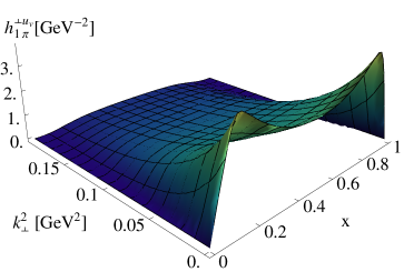
(a)	(b)	(c)

Figure 4: The Boer-Mulder function of the pion in the DY process from the LFCM at initial scale. (a) $h_{1,\pi}^{\perp u_{v}}(x,\boldsymbol{k}_{\perp}^{2})$ as function of $x$ and $\boldsymbol{k}^{2}_{\perp}$. (b) $h_{1,\pi}^{\perp u_{v}}$ as function of $\boldsymbol{k}^{2}_{\perp}$ for selected values of $x$ ($x=0.1$ solid curve, $x=0.3$ dotted curve, $x=0.5$ dashed curve). (c) The positivity relation (35) for the valence-$u$ quark in the pion as a function of $k_{\perp}$ at different values of $x$: $x$=0.2 (solid curve), $x=0.35$ (dashed curve) and $x$=0.5 (dotted curve).

In Fig. 4a we show the LFCM results for the Boer-Mulders TMD as function of $x$ and $\boldsymbol{k}^{2}_{\perp}$ with the sign as it is expected to appear in the DY process. The shape of the distribution is very similar to the unpolarized TMD. It is symmetric with respect to $x=1/2$, with a peak at $x\sim 0.1$, and is rapidly decreasing at larger $\boldsymbol{k}^{2}_{\perp}$, with a fall-off which is not Gaussian but can be approximated reasonably well by a Gaussian function. This is evident from Fig. 4b which displays the $\boldsymbol{k}^{2}_{\perp}$ dependence at selected values of $x$. The slope in $\boldsymbol{k}^{2}_{\perp}$ of the Boer-Mulders function is slightly steeper than that of the unpolarized TMD, in particular at larger values of $x$.

The next important test of the model calculation is posed by positivity Bacchetta:1999kz which requires that in the pion the unpolarized and Boer-Mulders TMD obey the following positivity relation, which holds flavor by flavor,

$$P_{{\rm BM}}^{q}(x,\boldsymbol{k}^{2}_{\perp})\equiv f_{1,\pi}^{q}(x,\boldsymbol{k}^{2}_{\perp})-\frac{k_{\perp}}{M_{\pi}}|h_{1,\pi}^{\perp\,q}(x,\boldsymbol{k}^{2}_{\perp})|\geq 0\;.$$ (35)

The model results for $P_{{\rm BM}}^{q}(x,\boldsymbol{k}^{2}_{\perp})$ at selected values of $x$ are plotted in Fig. 4c. We see that the inequality (35) is safely satisfied for $k_{\perp}\lesssim 0.2\,{\rm GeV}$ but violated for larger $k_{\perp}$. Calculations in effective nonperturbative model frameworks may provide some insights into the properties of TMDs for $k_{\perp}\ll\mu_{0}$, but the description of the region $k_{\perp}\sim{\cal O}(\mu_{0})$ is out of scope. Nevertheless, from the point of view of internal consistency, the non-compliance with (35) at large $k_{\perp}$ is of course unsatisfactory. This happens, to best of our knowledge, also in all presently available calculations of T-odd TMDs Kotzinian:2008fe . The general reasons for that can be traced back to an inconsistent treatment: T-odd TMDs are calculated to “first order of the expansion of the Wilson line,” whereas T-even TMDs like $f_{1}^{q}(x,\boldsymbol{k}^{2}_{\perp})$ are evaluated to “zeroth order” in that expansion. To preserve positivity the Wilson link expansion should be truncated consistently at the same order for both T-odd and T-even TMDs which enter the inequality (35) on the same footing Pasquini:2011tk .

From the point of view of practical applications, it is gratifying to observe that the inequality (35) is violated only in the region of small $x$ or large $k_{\perp}$ Kotzinian:2008fe ; Pasquini:2011tk , i.e. in a region of parameter space that is beyond the range of applicability of effective quark models. In particular, we convinced ourselves here that in the LFCM of the pion the non-compliance with inequalities in the extreme regions of the $(x,k_{\perp})$-space has no practical consequences for the description of physical processes, provided one uses the model within its range of applicability. The same observation was made in the case of the description of nucleon T-odd TMDs in the constituent quark model framework Pasquini:2011tk .

V.5 Comparison to results for Boer-Mulders functions from different models

It is instructive to compare the Boer-Mulders functions of pion and nucleon. Let us define the $(1/2)$- and $(1)$-transverse moments of the pion and proton Boer-Mulders functions as

$$h_{1,h}^{\perp(1/2)}(x)=\int d^{2}\boldsymbol{k}_{\perp}\frac{k_{\perp}}{2M_{h}}\,h_{1,h}^{\perp}(x,\boldsymbol{k}^{2}_{\perp}),\quad h_{1,h}^{\perp(1)}(x)=\int d^{2}\boldsymbol{k}_{\perp}\frac{\boldsymbol{k}^{2}_{\perp}}{2M^{2}_{h}}\,h_{1,h}^{\perp}(x,\boldsymbol{k}^{2}_{\perp}).$$ (36)

Owing to the appearance of hadron masses in the correlators defining the Boer-Mulders functions in Eq. (23), the magnitude of the $(1)$ moment of the pion Boer-Mulders function is artificially enhanced by a factor $\sim M_{p}/M_{\pi}$ with respect to the nucleon case. Therefore, in the following plots, we will rescale the results for the (1) moment of the proton Boer-Mulders function by that factor, in such a way that the comparison with the results for the pion is not distorted by the numerically very different values of pion and nucleon masses.

Fig. 5a compares the results for $h_{1,\pi}^{\perp(1/2)u_{v}}(x)$ obtained here and $h_{1,p}^{\perp(1/2)q_{v}}(x)$ obtained in Pasquini:2011tk . Similarly, Fig. 5b show the results for the (1) moment of the pion Boer-Mulders function in comparison with the corresponding results for valence quarks in the proton, rescaled by a factor $M_{p}/M_{\pi}$. In both cases, the distributions for the valence contribution in the proton and pion have comparable magnitude, but similarly to the case of the unpolarized PDF, the $x$ dependence is quite different. The sign of the pion Boer-Mulders function is consistent with the sign of the Boer-Mulders function of the proton Burkardt:2007xm , as obtained also in lattice calculations Engelhardt:2013nba , the MIT-bag model Lu:2012hh and spectator models Lu:2005rq ; Gamberg:2009uk . Interestingly, in comparison with other model calculations like the spectator model Lu:2005rq ; Gamberg:2009uk and MIT-bag model Lu:2012hh , the shape and the magnitude of $h_{1,\pi}^{\perp}$ from LFCM are quite different. Similar differences have been found also in the comparison of the model results for the proton Boer-Mulders function Pasquini:2010af ; Pasquini:2011tk . The LFCM predictions for the nucleon Boer-Mulders function favorably describe available SIDIS data Pasquini:2011tk . In Sec. VIII we will see that the LFCM predictions for the pion Boer-Mulders function provide a similarly satisfactory description of DY data.

(a)	(b)	(c)

Figure 5: (a) Comparison of $x\,h_{1}^{\perp(1/2)q_{v}}(x)$ in the DY process as functions of $x$ in pion and nucleon from LFCM approaches at initial scales. Solid line: $u_{v}$-distribution in pion, this work. Dotted (dashed) curve: $u_{v}$- ($d_{v}$-) distribution in proton, Ref. Pasquini:2008ax . (b) The results for $xh_{1\,{\rm DY}}^{\perp\,(1)}$ as function of $x$ . Solid curve: $u_{v}$-distribution in pion. Dotted (dashed) curve: $u_{v}$- ($d_{v}$)distribution in proton, from the LFCM of Ref. Pasquini:2011tk . The proton results are rescaled by a factor $M_{p}/M_{\pi}$. (c) The same as in Fig. 5b but at $Q^{2}=25$ GeV², obtained with approximate LO evolution from the LFCM results at the hadronic scale.

V.6 Estimating the $x$-evolution for the Boer-Mulders function

For phenomenological applications we will need the pion Boer-Mulders function from the LFCM evolved to experimentally relevant scales. This requires both, evolution in $x$ and transverse momentum. In this section we discuss the $x$-evolution (the evolution of the transverse-momentum dependence will be discussed in the next section.)

Recently, substantial progress on the evolution of TMDs has been achieved Collins-book ; Aybat:2011zv ; Aybat:2011ge ; Cherednikov:2007tw ; Bacchetta:2013pqa ; Echevarria:2012pw . However, the exact evolution equations for the Boer-Mulders function are still under study. At the present stage we have to resort to approximations in order take into account effects of scale dependence. To this aim, we will follow the same strategy as we adopted for the Boer-Mulders function of proton Pasquini:2011tk , and approximate the evolution of transverse moments of the Boer-Mulders function by using the evolution equations of the chiral-odd transversity distribution function in the nucleon (in a spin-zero hadron like pion there is of course no transversity distribution, but the pion Boer-Mulders originates from the same unintegrated chiral odd correlator).

To be more precise, we will evolve the (1)-moments of the Boer-Mulders functions. Such transverse moments appear naturally in transverse-momentum weighted azimuthal asymmetries, and it was argued that asymmetries weighted in this way are less affected by Sudakov effects Boer:2001he . It will be possible to ultimately judge the quality of this approximation only after the exact evolution equations are known. But we feel confident that the uncertainty introduced by this step in our theoretical study is not larger than the generic accuracy of the LFCM.

Fig. 5c show the results for (1)-moment $xh_{1\,{\rm DY}}^{\perp\,(1)}$ after approximate (transversity) LO-evolution from the initial scale in Eq. (2) to $Q^{2}=25$ GeV². For comparison we include also the results for the nucleon Boer-Mulders functions, rescaled by a factor $M_{p}/M_{\pi}$. As in the case of the unpolarized PDF, the effects of the evolution are sizable, producing a shift of the peak position towards smaller $x$ and reducing the magnitude of the distribution.

In Sec. VI we will use the model predictions to describe azimuthal asymmetries in DY in a LO treatment. For this purpose, we will use the results for $f_{1,\pi}(x)$ and $h_{1,\pi}^{\perp\,(1)}(x)$ LO evolved in $x$ to experimental scales – exactly and approximately, respectively, as described in Sec. V.3 and the present Sec. V.6. Before applying the model results to phenomenology, in the following section we will estimate the broadening of transverse momenta at the large scales typically probed in DY experiments.

VI The Drell-Yan process with unpolarized hadrons

In this Section we introduce the concepts required to describe the Drell-Yan process in the parton model taking into account transverse-momentum effects. Our treatment will be pragmatic and phenomenological.

VI.1 Kinematics, variables, conventions

Let $p_{1,2}$ denote the momenta of the incoming hadrons $h_{1,2}$, and let $l$, $l^{\prime}$ be the momenta of the outgoing lepton pair. The kinematics of the process is described by the center of mass energy square $s$, invariant mass of the lepton pair $Q$, rapidity $y$ or the Feynman variable $x_{F}$, and the variable $\tau$ which are defined and related to each other as

$$s=(p_{1}+p_{2})^{2}\,,\;\;\;q=l+l^{\prime}\,,\;\;\;Q^{2}=q^{2}\,,\;\;\;y=\frac{1}{2}\,\ln\frac{p_{2}\cdot q}{p_{1}\cdot q}=\frac{1}{2}\,\,\ln\frac{x_{1}}{x_{2}}\,,\;\;\;$$

$$x_{F}=x_{1}-x_{2}\,,\;\;\;\tau\equiv\frac{Q^{2}}{s}=x_{1}x_{2}\,.$$ (37)

In the parton model the $x_{i}$ denote the fractions of the hadron momenta $p_{i}$ carried by (respectively) the annihilating parton or anti-parton, and are given by (the $+$ signs refer to $x_{1}$, the $-$ signs $x_{2}$)

$$x_{1,2}=\pm\frac{x_{F}}{2}+\sqrt{\frac{x_{F}^{2}}{4}+\tau\;}=\sqrt{\tau}\,e^{\pm y}\;.$$ (38)

In the lab frame, where one hadron is a target or where both hadrons are beam particles, the produced lepton pair will in general have a three-momentum $\boldsymbol{q}=\boldsymbol{l}+\boldsymbol{l}^{\;\prime}\neq 0$. It is often convenient to analyze the data in a dilepton rest frame. There are various frames, including several dilepton rest frames, that are routinely used for data analyses, see Ref. McGaughey:1999mq ; Reimer:2007iy ; Arnold:2008kf ; Chang:2013opa ; Peng:2014hta for an overview. The differences between the different frames are of order ${\cal O}(q_{T}/Q)$. In the following we will work in the Collins-Soper frame, which is defined in Fig. 6, and use only data analyzed in that frame.

In this work we will consider pion-nucleus collisions. The used convention is such that $x_{1}$ describes the momentum fraction of the parton from $\pi^{-}$, while $x_{2}$ describes the momentum fraction of the parton from the nucleon bound in the nucleus. In order to describe nuclei with proton number $Z$ and neutron number $N$ we will neglect nuclear binding effects and assume that, for instance, $f_{1/\rm nucleus}^{u}=(Z/A)\,f_{1/\rm proton}^{u}+(N/A)\,f_{1/\rm neutron}^{u}$, where $A=N+Z$ denotes the mass number of the nucleus. The neglect of nuclear binding effects is a justified step for $q_{T}\lesssim 3\,{\rm GeV}$ Guanziroli:1987rp ; Bordalo:1987cs , which includes the kinematic region of interest for our study.

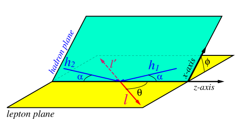
Figure 6: The definition of the angles $\theta$ and $\phi$ in the Collins-Soper frame. This frame is the center of mass frame of the produced leptons in which the hadrons are incoming symmetrically with respect to the $z$-axis (at an angle $\alpha$ in the figure) with the transverse momentum $q_{T}$.

VI.2 Structure functions in unpolarized DY

The angular distribution of the DY lepton pairs originating from collisions of unpolarized hadrons is given in the Collins-Soper frame by (see Fig. 6 for the definition of angles),

$$\frac{dN}{d\Omega}\equiv\frac{d\sigma}{d^{4}q\,d\Omega}\bigg{/}\frac{d\sigma}{d^{4}q}=\frac{3}{4\pi}\,\frac{1}{\lambda+3}\bigg{(}1+\lambda\cos^{2}\theta+\mu\sin 2\theta\cos\phi+\frac{\nu}{2}\sin^{2}\theta\cos 2\phi\bigg{)}\;.$$ (39)

In the notation of Ref. Arnold:2008kf the coefficients $\lambda$, $\mu$, $\nu$ can be expressed in terms of DY structure functions as follows

$$\lambda=\frac{F_{UU}^{1}-F_{UU}^{2}}{F_{UU}^{1}+F_{UU}^{2}}\,,\qquad\mu=\frac{F_{UU}^{\cos\phi}}{F_{UU}^{1}+F_{UU}^{2}}\,,\qquad\nu=\frac{2\,F_{UU}^{\cos 2\phi}}{F_{UU}^{1}+F_{UU}^{2}}\,.$$ (40)

The so-called Lam-Tung relation claims $\lambda+2\nu=1$, which reads in terms of structure functions $F_{UU}^{2}=2\,F_{UU}^{\cos 2\phi}$. This relation is exact if one treats the DY process to ${\cal O}(\alpha_{s})$ in the standard collinear factorization QCD framework Lam:1978pu ; Collins:1978yt . At ${\cal O}(\alpha_{s}^{2})$ the Lam-Tung relation is violated, though at a numerically negligible rate Mirkes:1994dp . However, DY data from pion-nucleus collisions show that it is strongly violated, calling for a nonperturbative leading-twist mechanism beyond collinear factorization. The Boer-Mulders effect provides such a mechanism Boer:1999mm . Alternative nonperturbative mechanisms to explain this observation have been proposed in Brandenburg:1993cj ; Brandenburg:1994wf ; Boer:2004mv ; Brandenburg:2006xu ; Nachtmann:2014qta .

VI.3 Parton model treatment

In a tree-level parton model approach including transverse parton momenta in the region $q_{T}\ll Q$ the structure functions $F_{UU}^{1}$ and $F_{UU}^{\cos 2\phi}$ are leading twist, $F_{UU}^{\cos\phi}$ is subleading twist, and $F_{UU}^{2}$ is a power-suppressed higher-twist effect proportional to $q_{T}^{2}/Q^{2}$. In such a treatment the transverse dilepton momenta $q_{T}$ arise from the convolutions of (“intrinsic”) transverse momenta of the partons as described through TMDs. The leading-twist structure functions in the unpolarized DY process are expressed in terms of TMDs through the following convolution integrals Arnold:2008kf

$$F_{UU}^{1}(x_{1},x_{2},q_{T}) = \frac{1}{N_{c}}\,\sum_{a}\,e_{a}^{2}\,\int d^{2}\boldsymbol{k}_{1\perp}\,d^{2}\boldsymbol{k}_{2\perp}\,\delta^{(2)}(\boldsymbol{q}_{T}-\boldsymbol{k}_{1\perp}-\boldsymbol{k}_{2\perp})\,f_{1,\pi}^{a}(x_{1},\boldsymbol{k}_{1\perp}^{2})\,f_{1,N}^{\bar{a}}(x_{2},\boldsymbol{k}_{2\perp}^{2})\,,$$ (41)

$$F_{UU}^{\cos(2\phi)}(x_{1},x_{2},q_{T}) = \frac{1}{N_{c}}\,\sum_{a}\,e_{a}^{2}\,\int d^{2}\boldsymbol{k}_{1\perp}\,d^{2}\boldsymbol{k}_{2\perp}\,\delta^{(2)}(\boldsymbol{q}_{T}-\boldsymbol{k}_{1\perp}-\boldsymbol{k}_{2\perp})\;\omega_{\rm BM}\;h_{1,\pi}^{\perp a}(x_{1},\boldsymbol{k}^{2}_{1\perp})_{\rm DY}\,h_{1,N}^{\perp\bar{a}}(x_{2},\boldsymbol{k}^{2}_{2\perp})_{\rm DY}\,,\;\;\;$$ (42)

$$\omega_{\rm BM} = \frac{2\big{(}\boldsymbol{q}_{T}\cdot\boldsymbol{k}_{1\perp}\big{)}\big{(}\boldsymbol{q}_{T}\cdot\boldsymbol{k}_{2\perp}\big{)}-q_{T}^{2}(\boldsymbol{k}_{1\perp}\cdot\boldsymbol{k}_{2\perp})}{M_{\pi}\,M_{N}\;q_{T}^{2}}\;,$$

where the sums go over $a=u,\,\bar{u},\,d,\,\bar{d}$, and, in principle, heavier flavors.

At this point it is important to recall that the parton model description is adequate and works reasonably well for some observables, but not for all. For instance, in order to describe absolute cross sections (even if averaged over transverse dilepton momenta), it is necessary to go to the NLO QCD-treatment of the process. We will work in a LO (“tree-level”) formalism and consider ratios of cross sections where “overall normalizations” tend to cancel out. Indeed, experience in various processes shows that different types of corrections may significantly affect absolute cross sections, but tend to cancel in cross section ratios. To quote just a few examples, we mention in this context the weak scale dependence of longitudinal spin asymmetries in DIS Kotikov:1997df , or the near cancellation of resummation effects of large double logarithmic QCD corrections in longitudinal spin asymmetries in SIDIS Koike:2006fn . In longitudinal and transverse spin asymmetries in DY higher order QCD corrections also tend to cancel Ratcliffe:1982yj ; Vogelsang:1992jn ; Boer:2006eq , and the same tendency is found for partonic threshold corrections Shimizu:2005fp . QCD corrections to polarization effects in $e^{+}e^{-}$ annihilation tend also to cancel Ravindran:2000rz . This is encouraging, but of course does not prove that higher order corrections will tend to cancel also for the cross section ratios considered in this work, and more theoretical work is needed to attest this point. We finally remark, that our parton model treatment does not consider the color entanglement effects discussed in Ref. Buffing:2013dxa .

VII The unpolarized TMDs in DY

The LFCM was shown to describe the $x$ dependence of $f_{1,h}$ with an accuracy of (10-30)$\,\%$ within the range of applicability of the model. (For pion see Sec. V, for nucleon see Ref. Lorce:2011dv .) In this section we will therefore focus entirely on the $k_{\perp}$ dependence.

VII.1 Gaussian approximation and estimate of $k_{\perp}$ broadening for $f^{a}_{1,h}(x,\boldsymbol{k}^{2}_{\perp})$

The LFCM predictions for the $k_{\perp}$ dependence of TMDs presented in Sec. V refer to a low scale of $\sim 0.5\,{\rm GeV}$, and cannot be applied directly to describe DY data which are typically taken in the region $Q\sim(4\mbox{--}9)\,{\rm GeV}$ between the $J/\psi$ and $\Upsilon$ resonances, or above the $\Upsilon$ resonance region. In order to estimate the $k_{\perp}$-evolution effects we shall resort to the Gaussian Ansatz, and proceed phenomenologically. The procedure is motivated and outlined below.

The DY cross section behaves like ${\rm d}\sigma/{\rm d}q_{T}^{2}\propto\exp(-q_{T}^{2}/\langle q_{T}^{2}\rangle)$ for $q_{T}\ll Q$ Cox:1982wy ; D'Alesio:2007jt ; Schweitzer:2010tt . This observation is the basis for the popularity of the Gaussian Ansatz to model the distributions of transverse parton momenta in hadrons. Although certainly oversimplifying, the phenomenological success of the Gaussian Ansatz indicates that it is a useful working assumption. We shall therefore recast the model predictions for TMD as follows

$$f_{1,h}^{a}(x,\boldsymbol{k}^{2}_{\perp})=f_{1,h}^{a}(x)\,\frac{\exp(-k_{\perp}^{2}/{\langle k_{\perp,\rm unp}^{2\;\,a/h}(x)\rangle})}{\pi\,{\langle k_{\perp,\rm unp}^{2\;\,a/h}(x)\rangle}}\;, {\langle k_{\perp,\rm unp}^{2\;\,a/h}(x)\rangle}=\frac{\int{\rm d}^{2}\boldsymbol{k}_{\perp}\;\boldsymbol{k}_{\perp}^{2}\,f_{1,h}^{a}(x,\boldsymbol{k}_{\perp}^{2})}{\int{\rm d}^{2}\boldsymbol{k}_{\perp}\;f_{1,h}^{a}(x,\boldsymbol{k}^{2}_{\perp})}\;,$$ (43)

where $f_{1,h}^{a}(x)$ is the unpolarized collinear parton distribution function.

Before describing in detail how we estimate $k_{\perp}$-evolution effects, let us comment on a feature concerning Eq. (43). In Sec. V we have seen that the model results for pion TMDs exhibit an approximate Gaussian behavior. The same was demonstrated in Boffi:2009sh ; Pasquini:2011tk for the nucleon case. In contrast to Refs. Boffi:2009sh ; Pasquini:2011tk (where predictions from the LFCM of the nucleon were applied to SIDIS phenomenology) in this work we do not take the Gaussian widths to be $x$-independent constants. Rather, in Eq. (43) we allow a more flexible parameterization with $x$-dependent Gaussian widths. This has the advantage of further improving the quality of the Gaussian approximation.

The exact evolution of the $k_{\perp}$ dependence of the unpolarized TMD is known in the Collins-Soper-Sterman (CSS) formalism, which provides a framework for a quantitative description of transverse-momentum broadening effects with increasing energies. The underlying physical picture is that with increasing energy gluon radiation broadens the “initial” (or “intrinsic”) parton transverse momentum. There is no practical or theoretical way to separate “nonperturbative intrinsic” and “perturbative gluon-radiation” effects. However, from a phenomenological point of view, there is no need for that: both effects are collectively parametrized in the effective parameters in Eq. (43), provided one pays due attention to apply this effective description to the region of low transverse momenta $q_{T}\ll Q$ D'Alesio:2007jt ; Schweitzer:2010tt . In order to estimate this effective broadening of the Gaussian widths we shall use the results from Schweitzer:2010tt .

In principle one could directly work within the CSS formalism. However, the CSS-formalism has not yet been established for the Boer-Mulders effect. Moreover, even in the unpolarized case, it has not yet been studied whether one can use the CSS formalism starting from a scale as low as in Eqs. (2) and (3). In this work we therefore prefer to use the effective description of Schweitzer:2010tt to estimate $k_{\perp}$-evolution effects, which requires to use the Gaussian Ansatz, as done in Eq. (43). The details of this step will be described below.

Let us now turn our attention to the description of the transverse parton momenta in DY. We discuss first the mean transverse momenta of the produced lepton pairs (see Eqs. (37) and (38) for the relation of $x_{F}$ with $x_{1,2}$) defined as

$$\langle q_{T}^{2}(x_{F},s)\rangle=\frac{\int d^{2}q_{T}\;q_{T}^{2}\,F_{UU}^{1}(x_{1},x_{2},q_{T})}{\int d^{2}q_{T}\,F_{UU}^{1}(x_{1},x_{2},q_{T})}\>.$$ (44)

It is important to notice that in a LO formalism the energy (or scale) dependence is introduced by using parton distributions (LO-) evolved to the relevant scale, and using appropriately broadened Gaussian widths. We also notice that $\langle q_{T}^{2}(x_{F},s)\rangle$ is a ratio of observables, i.e. amenable to the description in a parton model approach thanks to the approximate cancellation of higher order QCD effects, as argued in Sec. VI.3.

When using the Gaussian Ansatz in a tree-level parton model approach, the $\langle q_{T}^{2}\rangle$ is given by the sum of the Gaussian widths of the unpolarized TMDs of the nucleon and pion. (In general this would hold only if the Gaussian widths were flavor independent. In the LFCM, where sea quarks are absent, it also holds because only one flavor contributes to the production of the lepton pair, namely a valence $\bar{u}$ from the $\pi^{-}$ and a valence $u$ in the proton annihilate.)

If we used the model results discussed in Sec. V at their face value to estimate $\langle q_{T}^{2}\rangle$ we would strongly underestimate the data. This is not surprising as the model results have to be evolved. In order to estimate evolution effects, we add an energy-dependent constant $\langle\delta k_{\perp}^{2}(s)\rangle$ such that

$$\langle q_{T}^{2}(x_{F},s)\rangle={\langle k_{\perp,\rm unp}^{2\;\,\bar{u}/\pi^{-}}(x_{1})\rangle}+{\langle k_{\perp,\rm unp}^{2\;\,u/N}(x_{2})\rangle}+\langle\delta k_{\perp,\rm unp}^{2}(s)\rangle\;.\;\;\;$$ (45)

The energy dependence of $\langle q_{T}^{2}\rangle$ enters only through $\langle\delta k_{\perp,\rm unp}^{2}(s)\rangle$ which provides the amount of transverse-momentum broadening at given $s$. The variation of dilepton momenta with $s$ was investigated phenomenologically in Cox:1982wy ; Schweitzer:2010tt . These studies allow us to estimate the amount of $k_{\perp}$ broadening required in our approach to be

$$\langle\delta k_{\perp,\rm unp}^{2}(s)\rangle=\delta A_{\rm unp}+B_{\rm unp}\;s\;,\;\;\;\delta A_{\rm unp}=0.4\,{\rm GeV}^{2}\,,\;\;\;B_{\rm unp}=2.6\times 10^{-3}\,.$$ (46)

It is important to stress that $\langle\delta k_{\perp,\rm unp}^{2}(s)\rangle$ constitutes the accumulated $k_{\perp}$ broadening in both pion and nucleon. Notice that $\langle\delta k_{\perp,\rm unp}^{2}(s)\rangle$ could also depend on $x_{F}$ or other variables besides $s$, but we disregard this possibility here. Finally, one should stress that that the linear broadening indicated in (46) is valid only in a narrow $s$-range Cox:1982wy ; Schweitzer:2010tt . When considering broader energy ranges up to collider energies the increase is $\log s$ Landry:2002ix rather than linear.

VII.2 Comparison to data

With the empirical estimate of $k_{\perp}$-broadening effects in Sec. VII.1, the model results yield a good description of DY data in the region $s\sim(50\mbox{--}600)\,{\rm GeV}^{2}$ studied in Refs. Cox:1982wy ; Schweitzer:2010tt . We present two examples to illustrate this.

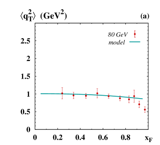
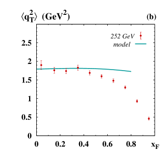
Figure 7: The mean dimuon transverse-momentum square $\langle q_{T}^{2}\rangle$ vs. $x_{F}$ from the Fermilab E615 experiment taken with respectively (a) $80\,{\rm GeV}$ Palestini:1985zc and (b) $252\,{\rm GeV}$ Conway:1989fs $\pi^{-}$ beams impinging on tungsten targets. The theoretical curves are the result from LFCM obtained in this work with a phenomenological estimate for transverse-momentum broadening, see Eqs. (45) and (46).

Fig. 7 shows how our approach describes Fermilab E615 data on $\langle q_{T}^{2}(x_{F})\rangle$ of Drell-Yan lepton pairs produced in collisions of $80\,{\rm GeV}$ and $252\,{\rm GeV}$ $\pi^{-}$ beams impinging on tungsten targets Palestini:1985zc ; Conway:1989fs , which corresponds respectively to $s\simeq 150\,{\rm GeV}^{2}$ and $473\,{\rm GeV}^{2}$. We obtain a good description of the $80\,{\rm GeV}$ data Palestini:1985zc in the region $0.2\leq x_{F}\lesssim 0.8$. The $252\,{\rm GeV}$ data are well described for $0\leq x_{F}\lesssim 0.5$. Considering the generic accuracy $\sim(10\mbox{--}30)\,\%$ of the LFCM, the description of these data in the region $0.5\lesssim x_{F}\lesssim 0.7$ can be still considered satisfactory. However, beyond $x_{F}\gtrsim 0.7$ the approach breaks down. This is not a failure of the model (which admittedly is not applicable at small- or large-$x$), but of the TMD approach in general. The reason is as follows. At large $x_{F}$ the breakdown of the description of the DY process in terms of parton distribution functions is expected. The limit $x_{F}\rightarrow 1$ corresponds to large $x_{1}$ in the pion (and small $x_{2}$ in the nucleon). As $x_{1}\rightarrow 1$ the $\bar{u}$ from the $\pi^{-}$ is far off-shell, and more appropriately described in terms of the pion distribution amplitude Berger:1979du . While this so-called Berger-Brodsky effect provides a unique opportunity to access information on the pion distribution amplitude Bakulev:2007ej , from the point of view of the TMD description of the DY process it is a power correction, which dominates as one approaches the limit $x_{F}\rightarrow 1$ of the available phase space. Interestingly the Gaussian Ansatz itself still works even for $x_{F}\gtrsim 0.7$ Schweitzer:2010tt . In principle one could continue using the TMD description, at least in some parts of the large-$x_{F}$ region. This would require narrower $\langle q_{T}^{2}(x_{F})\rangle$. The $x_{F}$ dependence of $\langle q_{T}^{2}(x_{F})\rangle$ implied by the LFCM through the $x$ dependence of the Gaussian widths in Eq. (43) is not sufficient for that, but one could introduce an adequate $x_{F}$ dependence of the transverse-momentum broadening $\langle\delta k_{\perp,\rm unp}^{2}(s)\rangle$ in addition to its $s$ dependence. In this work we shall refrain from such attempts, stick to our $x_{F}$-independent description of transverse-momentum broadening in Eqs. (45) and  (46), and keep in mind that this description has limitations at large $x_{F}$.

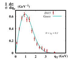
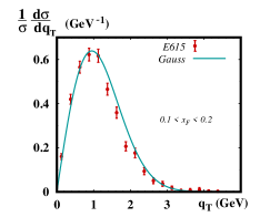
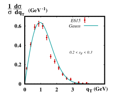
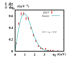
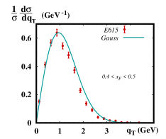
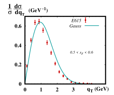
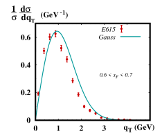
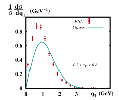
Figure 8: The normalized cross section $(1/\sigma)\,({\rm d}\sigma(q_{T})/{\rm d}q_{T})$ as functions of $q_{T}$ in different $x_{F}$-bins. The data are from Ref. Conway:1989fs . The theoretical curves are from the LFCM with transverse-momentum broadening effects estimated according to Eqs. (45) and  (46). The description of the data is very good in the region $0\leq x_{F}\leq 0.5$, and it is still acceptable for $0.5\leq x_{F}\lesssim 0.7$. For $x_{F}\gtrsim 0.7$ the description breaks down, because the TMD approach is not applicable and higher twist effects become relevant.

The observable $\langle q_{T}^{2}(x_{F})\rangle$ shown in Fig. 7 is the result of averaging over DY pair momenta. It is of importance to demonstrate that our approach works also for observables depending on $q_{T}$. For that we consider the data from the E615 experiment Conway:1989fs shown in Fig. 8 on the normalized cross sections, which we define for brevity as

$$\frac{1}{\sigma}\,\frac{{\rm d}\sigma(q_{T})}{{\rm d}q_{T}}\equiv\frac{{\rm d}^{2}\sigma(q_{T},x_{F})}{{\rm d}q_{T}\,{\rm d}x_{F}}\Biggl{/}\frac{{\rm d}\sigma(x_{F})}{{\rm d}x_{F}}=\frac{2\pi\,q_{T}\,\langle F_{UU}^{1}(x_{1},x_{2},q_{T})\rangle}{\langle F_{UU}^{1}(x_{1},x_{2})\rangle},$$ (47)

where $\langle\,\cdots\,\rangle$ denote averages over $x_{F}$ in certain bins, and $\sigma$ in the first term of Eq. (47) is a short-cut notation for the differential cross section ${\rm d}\sigma/{\rm d}x_{F}$. The normalization is such that one obtains unity after integrating over $q_{T}$ in Eq. (47). Using the Gaussian Ansatz, the structure functions are given by

$$F_{UU}^{1}(x_{1},x_{2},q_{T}) = \frac{1}{N_{c}}\,\sum_{a}e_{a}^{2}f_{1,\pi}^{a}(x_{1})\,f_{1,N}^{\bar{a}}(x_{2})\,\frac{\exp(-{q_{T}^{2}}/\langle q_{T}^{2}\rangle)}{\pi\langle q_{T}^{2}\rangle}\;,$$ (48)

$$F_{UU}^{1}(x_{1},x_{2}) = \frac{1}{N_{c}}\,\sum_{a}e_{a}^{2}f_{1,\pi}^{a}(x_{1})\,f_{1,N}^{\bar{a}}(x_{2})\;.$$ (49)

Notice that $F_{UU}^{1}(x_{1},x_{2},q_{T})$ in Eq. (48) depends on the Gaussian model, but after integrating out transverse momenta one obtains the model-independent structure function $F_{UU}^{1}(x_{1},x_{2})=\int{\rm d}^{2}q_{T}\,F_{UU}^{1}(x_{1},x_{2},q_{T})$ in Eq. (49). The data refer to $4.05\leq Q/{\rm GeV}\leq 8.55$ and were taken with a 252 GeV $\pi^{-}$ beam impinging on a nuclear (tungsten) target Conway:1989fs . Thus $s\simeq 473\,{\rm GeV}^{2}$ in this experiment. Strictly speaking we could only retrieve E615 data on ${\rm d}^{2}\sigma/({\rm d}q_{T}\,{\rm d}x_{F})$ from Ref. Stirling:1993gc , and estimated the differential cross sections ${\rm d}\sigma/{\rm d}x_{F}$ ourselves, to obtain the normalized data in Fig. 8. We are confident that the data shown in Fig. 8 are normalized with an accuracy of $10\,\%$, which is comparable or better than the accuracy of the LFCM. (We recall that we work in a LO approach. Thus, we could have alternatively studied the $q_{T}$ dependence of the differential cross sections ${\rm d}^{2}\sigma/({\rm d}q_{T}\,{\rm d}x_{F})$ fixing the overall normalizations “by hand,” or estimating “K-factors.” Both alternatives are not more rigorous than our treatment.)

Fig. 8 shows that the description of the $q_{T}$ dependence of the normalized cross sections works very well in the region $0\leq x_{F}\leq 0.5$, is still reasonably good for $0.5\leq x_{F}\lesssim 0.7$, but for $x_{F}\gtrsim 0.7$ it clearly breaks down, which is not surprising given our earlier findings concluded from Fig. 7 and the expectations from QCD for $x_{F}\rightarrow 1$ Berger:1979du . It is important to stress that we do not only expect limitations of the approach at large $x_{F}$, but in particular also at large $q_{T}$, where the Gaussian Ansatz is at variance with QCD which predicts a power-like decay Bacchetta:2008xw . These limitations cannot be seen in Fig. 8. We therefore present a logarithmic plot of the E615 data Conway:1989fs on the normalized cross section in Fig. 9 which demonstrates that the Gaussian description is applicable for $q_{T}\lesssim(2\mbox{--}3)\,{\rm GeV}$ but not beyond that.

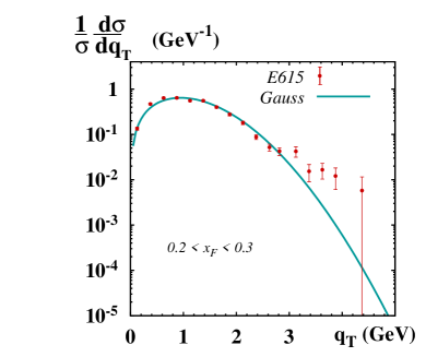
Figure 9: The normalized cross section $(1/\sigma)\,({\rm d}\sigma(q_{T})/{\rm d}q_{T})$ as function of $q_{T}$ for $0.2\leq x_{F}\leq 0.3$. The data are from Ref. Conway:1989fs . The theoretical curves are from the LFCM with transverse-momentum broadening effects estimated according to Eqs. (45, 46). The logarithmic plot shows the limitation of the Gaussian description which works well for $q_{T}\lesssim(2\mbox{--}3)\,{\rm GeV}$.

Since $4.05\leq Q/{\rm GeV}\leq 8.55$ and we need $q_{T}\ll Q$ for the TMD factorization to be applicable, one certainly cannot expect the approach to work beyond $q_{T}\lesssim(2\mbox{--}3)\,{\rm GeV}$. In Fig. 9 we limit ourselves to showing the data in the bin $0.2\leq x_{F}\leq 0.3$ only, because this $x_{F}$-bin shows the limitations of the $q_{T}$-description most clearly. The data sets from Conway:1989fs in the other $x_{F}$-bins shown in the Fig. 8 happen to be less accurate at larger $q_{T}$ and show deviations from the Gaussian Ansatz less clearly. Depending on the energy, the Gaussian model was shown to work satisfactorily in DY up to $q_{T}\lesssim(2\mbox{--}3)\,{\rm GeV}$ also in Schweitzer:2010tt .

At this point it is worth recalling that we neglect nuclear binding effects, which is justified for $q_{T}\lesssim 3\,{\rm GeV}$ Guanziroli:1987rp ; Bordalo:1987cs . Thus, nuclear effects become important only beyond the range of $q_{T}$ we are interested in. Moreover, since in the LFCM the ${\langle k_{\perp,\rm unp}^{2\;\,}(x)\rangle}$ are equal for $u$- and $d$-quarks in protons and neutrons, we do not need to distinguish protons and neutrons in the tungsten target.

To summarize, a parton model description of cross section ratios in DY with the LFCM predictions for pion and nucleon unpolarized TMDs with the phenomenological estimate of transverse-momentum broadening effects in Eqs. (45) and  (46) works well for $s\sim(50\mbox{--}600)\,{\rm GeV}^{2}$ in the regions of $q_{T}\lesssim(2\mbox{--}3)\,{\rm GeV}$ and $x_{F}\lesssim(0.7\mbox{--}0.8)$. Although the LFCM has its own limitations, this is the range of applicability of the TMD approach expected on general grounds, and we shall keep it in mind when embarking on the description of the Boer-Mulders effect in DY in the next section.

VIII Boer-Mulders effect in DY

In this section we describe the Boer-Mulders effect in the DY process. The treatment is in large part parallel to the discussion of the unpolarized TMDs in Sec. VII.

VIII.1 Gaussian approximation and estimate of $k_{\perp}$ broadening for $h^{\perp a}_{1,h}(x,\boldsymbol{k}^{2}_{\perp})$

In analogy to the unpolarized TMDs in Eq. (50), also in the case of the Boer-Mulders functions it is convenient to recast the model predictions in terms of a Gaussian Ansatz as follows

$$h_{1,h}^{\perp a}(x,\boldsymbol{k}^{2}_{\perp})=h_{1,h}^{\perp a}(x)\,\frac{\exp(-k_{\perp}^{2}/{\langle k_{\perp,\rm BM}^{2\;\,a/h}(x)\rangle})}{\pi\,{\langle k_{\perp,\rm BM}^{2\;\,a/h}(x)\rangle}}\;, {\langle k_{\perp,\rm BM}^{2\;\,a/h}(x)\rangle}=\frac{\int{\rm d}^{2}\boldsymbol{k}_{\perp}\;\boldsymbol{k}_{\perp}^{2}\,h_{1,h}^{\perp a}(x,\boldsymbol{k}^{2}_{\perp})}{\int{\rm d}^{2}\boldsymbol{k}_{\perp}\;h_{1,h}^{\perp a}(x,\boldsymbol{k}^{2}_{\perp})}\;.$$ (50)

The model results for $h_{1,h}^{\perp a}(x,\boldsymbol{k}^{2}_{\perp})$ at the initial scale exhibit an approximate Gaussian $k_{\perp}$-behavior, see Fig. 4b in this work for pion and Boffi:2009sh for nucleon. This is well approximated by Eq. (50) thanks to the flexible $x$-dependent Gaussian width. Moreover, also in the case of the Boer-Mulders functions the Gaussian Ansatz will facilitate the estimate of transverse-momentum broadening effects, as described below.

We remark that $h_{1,h}^{\perp a}(x)=\int{\rm d}^{2}\boldsymbol{k}_{\perp}\,h_{1,h}^{\perp a}(x,\boldsymbol{k}^{2}_{\perp})$, though well-defined in models, would have an involved QCD definition because one should “divide out” a power of transverse momentum from the correlator in Eq. (23). However, this quantity appears here merely as an “intermediate-step construct” and will be eliminated in favor of the (1)-moment of the Boer-Mulders function in the final expression. We remark that treatments of the Boer-Mulders effect in DY in the Gaussian Ansatz were reported e.g. in Refs. Zhang:2008nu ; Barone:2010gk , though from our point of view the used Gaussian widths were sometimes chosen unacceptably small.

Using the Gaussian Ansatz (50), one can analytically evaluate the convolution integral in the structure function (42). There are “infinitely many” possible ways to express the result. We choose to write it in terms of (1)-moments of the Boer-Mulders function as follows

$$F_{UU}^{\cos(2\phi)}(x_{1},x_{2},q_{T}) = \frac{1}{N_{c}}\,\sum_{a}e_{a}^{2}h_{1,\pi}^{\perp(1)a}(x_{1})_{\rm DY}\,h_{1,N}^{\perp(1)\bar{a}}(x_{2})_{\rm DY}\;\frac{4M_{\pi}M_{N}}{\langle q_{T}^{2}\rangle_{\rm BM}}\;\,\frac{q_{T}^{2}\,\exp\big{(}-{q_{T}^{2}}/\langle q_{T}^{2}\rangle_{\rm BM})}{\pi\langle q_{T}^{2}\rangle^{2}_{\rm BM}}\;,$$ (51)

$$F_{UU}^{\cos(2\phi)}(x_{1},x_{2}) = \frac{1}{N_{c}}\,\sum_{a}e_{a}^{2}h_{1,\pi}^{\perp(1)a}(x_{1})_{\rm DY}\,h_{1,N}^{\perp(1)\bar{a}}(x_{2})_{\rm DY}\;\frac{4M_{\pi}M_{N}}{\langle q_{T}^{2}\rangle_{\rm BM}}\;,$$ (52)

$$\langle q_{T}^{2}(x_{1},x_{2},s)\rangle_{\rm BM} = {\langle k_{\perp,\rm BM}^{2\;\,a/\pi}(x_{1})\rangle}+{\langle k_{\perp,\rm BM}^{2\;\,\bar{a}/N}(x_{2})\rangle}+\langle\delta k_{\perp,\rm BM}^{2}(s)\rangle\;.$$ (53)

One could also use $h_{1,h}^{\perp a}(x)$ or $h_{1,h}^{\perp(1/2)a}(x)$, or any other moment $h_{1,h}^{\perp(n)a}(x)$ defined analogously to Eq. (36), in order to express the structure functions in Eqs. (51) and (52). From the point of view of the Gaussian model, all such expressions would be equally acceptable. From phenomenological point of view, our choice in Eqs. (51) and (52) is preferred in the sense that this is the only case, where one deals with a single parameter, $\langle\delta k_{\perp,\rm BM}^{2}(s)\rangle$, describing the accumulated $k_{\perp}$ broadening of the pion and nucleon Boer-Mulders functions. All other choices would require to explicitly estimate the $k_{\perp}$ broadenings of the separate pion and nucleon Gaussian widths ${\langle k_{\perp,\rm BM}^{2\;\,a/h}(x)\rangle}$.

We find a good description of data Guanziroli:1987rp ; Conway:1989fs on the $q_{T}$ dependence of the Boer-Mulders effect in DY with

$$\langle\delta k_{\perp,\rm BM}^{2}(s)\rangle=1.3\,{\rm GeV}^{2}\;\;\;\mbox{at}\;\;\;s\approx\mbox{(470--540)\,GeV${}^{2}$}$$ (54)

in the range of $q_{T}$ up to (2–3) GeV in which the Gaussian Ansatz was shown to be applicable for unpolarized TMDs in Sec. VII.2. DY data on the Boer-Mulders effect are available also for smaller center-of-mass energies $s$ Badier:1981ti ; Palestini:1985zc ; Falciano:1986wk ; Guanziroli:1987rp ; Conway:1989fs . But we observe that we cannot describe these data using Eqs. (51) and (52). More precisely, descriptions of the data at smaller $s$ are possible, but in a more limited range $q_{T}\lesssim 1$ GeV. We also found that different prescriptions to describe the structure function, say in terms of $h_{1,h}^{\perp a}(x)$ or $h_{1,h}^{\perp(1/2)a}(x)$, do not yield better descriptions.

These observations should not come as a surprise. None of such Gaussian Ansatz descriptions can be expected to adequately describe the true QCD scale dependence of the Boer-Mulders functions. However, as we will show in the next section, the Gaussian Ansatz is useful in a specific range of $s$ and $q_{T}$ with the understanding that $q_{T}\ll Q$. Only after the full CSS-evolution for the the Boer-Mulders functions will be available, it will be possible to undertake an attempt to describe Boer-Mulders data at all energies. Furthermore, it is important to compare the value of $\langle\delta k_{\perp,\rm BM}^{2}(s)\rangle$ in Eq. (54) with the broadening $\langle\delta k_{\perp,\rm unp}^{2}(s)\rangle=$ (1.6–1.8) GeV² of unpolarized TMDs in the same range of $s$. The accumulated $k_{\perp}$ broadening of the unpolarized TMDs is larger than that of the Boer-Mulders functions. This is a necessary (cf. Footnote 1) and, in our case, numerically also sufficient condition to comply with positivity.

VIII.2 Comparison to data

With the descriptions of the unpolarized structure function in Eqs. (45) and (49) and the Boer-Mulders structure function in Eqs. (51)–(54) we are now in the position to evaluate the coefficient $\nu$ in the angular distribution of the DY cross section in the Collins-Soper frame as defined through Eqs. (39) and (40).

We will compare to the data from the NA10 CERN experiment Guanziroli:1987rp and the E615 Fermi Lab experiment Conway:1989fs . In both experiments secondary $\pi^{-}$ beams were collided with nuclear targets. In the NA10 experiment Guanziroli:1987rp several beam energies were used. We will focus on the NA10 data taken with 286 GeV $\pi^{-}$ beams impinging on a tungsten or deuterium targets. The covered range of $Q$ was $4.0<Q<8.5\,{\rm GeV}$ and $Q>11\,{\rm GeV}$ to remove the influence of the $J/\psi$- and $\Upsilon$-resonance regions. In order to discard the Berger-Brodsky higher twist effect Berger:1979du the cut $x_{1}<0.7$ was imposed. In the E615 Fermi Lab experiment Conway:1989fs a 252 GeV $\pi^{-}$ beam was collided with a tungsten target, and the kinematic region $4.05<Q<8.55\,{\rm GeV}$ between the $J/\psi$- and $\Upsilon$-resonances was covered with $0.2<x_{1}<1$. For our theoretical calculation we assume for simplicity $\langle Q^{2}\rangle=25\,{\rm GeV}^{2}$ as typical hard scale in both experiments.

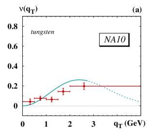
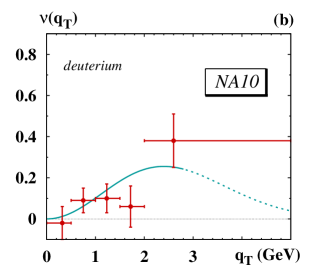
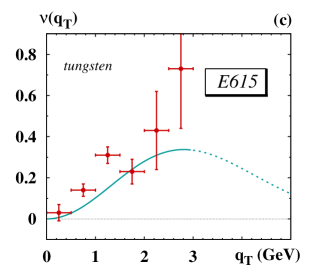
Figure 10: The coefficient $\nu$ in the $\pi^{-}$-nucleus DY angular distribution as function of $q_{T}$. The data are from the NA10 CERN experiment with $E_{\rm beam}=286\,{\rm GeV}$ using tungsten (a) and deuterium (b) targets Guanziroli:1987rp , and the E615 Fermi Lab experiment with $E_{\rm beam}=252\,{\rm GeV}$ using a tungsten target Conway:1989fs . The theoretical curves are obtained using the LFCM predictions for the pion Boer-Mulders function obtained here, and the analog nucleon predictions from Pasquini:2011tk . The solid (dotted) lines indicate where the TMD approach is applicable (not applicable).

Let us first discuss the $q_{T}$ dependence of the coefficient $\nu$. In the observable $\nu(q_{T})$ the model input determines the overall normalization, while the $q_{T}$ dependence is dictated by the Gaussian Ansatz with the estimated $k_{\perp}$ broadening of the Boer-Mulder functions in Eqs. (51) and (54). In fact, more than testing the LFCM predictions, this comparison shows that the use of the Gaussian Ansatz for the Boer-Mulders function with the estimated broadening (54) is compatible with data, as can be seen in Fig. 10.

Several comments are in order. First, the NA10 tungsten data shown in Fig. 10a have a 10-times larger statistics than the NA10 deuterium data in Fig. 10b. Within the statistical uncertainty of the data, no significant nuclear dependence was observed Guanziroli:1987rp . We exploited this observation when we defined our simplistic approach to estimate nuclear TMDs in Sec. VI.1. Second, there seems to be a tendency in our approach to slightly overestimate the tungsten data from NA10 in Fig. 10a, and to slightly underestimate the tungsten data from E615 in Fig. 10c. The effect is not statistically significant. If it was, an explanation for that could be the fact that in the E615 data the Berger-Brodsky effect was included ($x_{1}<1$) but not in the NA10 data ($x_{1}<0.7$). Indications for the Berger-Brodsky effect were seen in the E615 experiment Conway:1989fs . The slightly different energies in the two experiments could also play a role. Third, in Sec. VII.2 we learned that a Gaussian Ansatz for unpolarized TMDs works well in the region $q_{T}\lesssim\mbox{(2--3)}\,{\rm GeV}$, but breaks down beyond that. Our descriptions of $\nu(q_{T})$ in Fig. 10 are therefore certainly not valid for $q_{T}\gtrsim 3\,{\rm GeV}$ and we have emphasized this region with dotted lines. Clearly, in the region $q_{T}\lesssim\mbox{(2--3)}\,{\rm GeV}$ (indicated by solid lines) our description of $\nu(q_{T})$ is compatible with data. Forth, it should be noted that the TMD approach in general requires $q_{T}\ll Q$. Thus, our results in Fig. 10 indicate that in the range $s\approx\mbox{(470--540)\,GeV${}^{2}$}$ $\nu(q_{T})$ can be well described in the TMD approach with the Gaussian Ansatz. Finally, we remark that our results safely comply with the model-independent positivity bound $|\frac{\nu}{2}|\leq 1$.

Next, we turn our attention to the $x_{1}$ dependence of the coefficient $\nu$ shown in Fig. 11. We recall that $x_{1}$ corresponds to the momentum fraction carried by the parton which originates from the pion. We use this variable here, because it is the only common kinematical variable (besides $q_{T}$) used to analyze data in both experiments Guanziroli:1987rp ; Conway:1989fs . The observable $\nu(x_{1})$ provides a more stringent test of the model results, in the sense that the shapes of the theoretical curves in Fig. 11 are directly dictated by the LFCM predictions, although their overall normalizations are influenced through Eq. (52) by the choice of the parameter $\langle\delta k_{\perp,\rm BM}^{2}(s)\rangle$ in Eq. (54).

The comparison with the data in Fig. 11 is satisfactory. The most precise data set, namely the NA10 tungsten data in Fig. 11a, may indicate that our model results somewhat overshoot the data in the region around $x_{1}\sim 0.6$, but the effect is not significant. Even if it was, one should recall that the typical accuracy of the LFCM in applications to TMD phenomenology is (10–30)$\,\%$ Boffi:2009sh ; Pasquini:2011tk . The NA10 deuterium data Guanziroli:1987rp in Fig. 11b and the E615 tungsten data Guanziroli:1987rp ; Conway:1989fs in Fig. 11c have larger error bars, and our model results are compatible with them in the entire region of $x_{1}$.

It is important to keep in mind that the TMD approach is not applicable in the full range of $x_{1}$. In Sec. VII.2 we have seen that we can describe well the E615 data Conway:1989fs on the (normalized) DY cross sections for $x_{F}\lesssim 0.7$, but not in the region $x_{F}\gtrsim 0.7$, where the Berger-Brodsky effect becomes increasingly significant. In the kinematics of the NA10 and E615 experiments this $x_{F}$ region corresponds to $x_{1}\gtrsim 0.76$, and we have indicated this region by dotted lines in Fig. 11. The Berger-Brodsky effect is not prominent in the NA10 data shown in Figs. 11a and 11b. (Notice that the region of $x_{1}>0.7$ was excluded in the NA10 analysis of $\nu$ as function of $q_{T}$ which we discussed in Fig. 10.) However, there is an indication of this effect in E615 data shown in Fig. 11c.

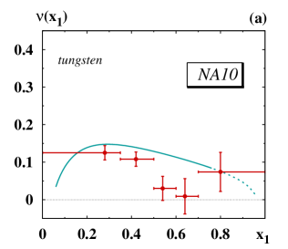
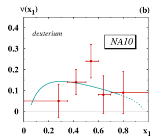
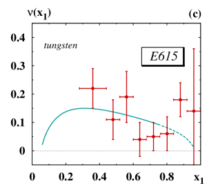
Figure 11: The coefficient $\nu$ in the $\pi^{-}$-nucleus DY angular distribution as function of $x_{1}$. The data are from the NA10 CERN experiment with $E_{\rm beam}=286\,{\rm GeV}$ using tungsten (a) and deuterium (b) targets Guanziroli:1987rp , and the E615 Fermi Lab experiment with $E_{\rm beam}=252\,{\rm GeV}$ using a tungsten target Conway:1989fs . The theoretical curves are obtained using the LFCM predictions for the pion Boer-Mulders function obtained here, and the corresponding nucleon predictions from Pasquini:2011tk . The solid (dotted) lines indicate where the TMD approach is applicable (not applicable).

To conclude, we observe that the predictions from the LFCM for the pion Boer-Mulders functions, from this work, and nucleon, from Pasquini:2011tk , are in good agreement with the NA10 and E615 data taken at $s\approx\mbox{(470--540)\,GeV${}^{2}$}$ Guanziroli:1987rp ; Conway:1989fs . The good agreement is based also on our use of the Gaussian Ansatz in the TMD factorization approach, and the chosen method to estimate $k_{\perp}$-broadening effects, which corresponds to estimating CSS-evolution effects.

IX Summary and Outlook

In this work we studied the structure of the pion, as described in terms of the leading twist TMDs $f_{1,\pi}(x,\boldsymbol{k}^{2}_{\perp})$ and $h_{1,\pi}^{\perp}(x,\boldsymbol{k}^{2}_{\perp})$, using a light-front constituent model where the pion is described in terms of the minimal Fock-state component consisting of a quark and antiquark. In a first step we determined the initial scale of this constituent approach to the pion, following a similar procedure commonly used in hadronic models with effective valence degrees of freedom. The resulting initial scale is about $\mu_{0}\sim 0.5\,{\rm GeV}$ and numerically similar to the initial scale in the case of the of constituent approach of the nucleon Boffi:2009sh , supporting the validity of the constituent approach.

The $q\bar{q}$ LFWF of the pion was shown to involve two independent amplitudes describing the different orbital angular momentum components of the constituent quark and antiquark in the pion state Burkardt:2002uc ; Ji:2003yj . In this work we derived a model-independent representation of leading-twist pion TMDs in terms of overlaps of light-front amplitudes which reveals the role of the different orbital angular momentum components for the structure of the pion. We applied these expressions to a specific model, which has been successfully employed to describe the pion electromagnetic form factor Schlumpf:1994bc ; Chung:1988mu . Our predictions for the pion TMDs are in qualitative agreement with results from spectator and bag models Lu:2004hu ; Burkardt:2007xm ; Gamberg:2009uk ; Lu:2012hh and lattice QCD Engelhardt:2013nba . We then evolved the model result for the collinear valence pion distribution function from the low hadronic scale to experimentally relevant scales, and demonstrated that it is in good agreement with available parametrizations. We observed that the $k_{\perp}$ dependence of the model TMDs is not exactly Gaussian, but can be usefully approximated by a Gaussian Ansatz. In comparison with the model results for the nucleon Boer-Mulders function Pasquini:2010af ; Pasquini:2011tk , we confirm that in LFCM approaches “all Boer-Mulders functions are alike,” in the qualitative sense of Ref. Burkardt:2007xm .

As a phenomenological application, we studied the pion-nucleus induced Drell-Yan process. We re-expressed the model results in terms of an effective Gaussian Ansatz for the $k_{\perp}$ dependence of TMDs, which is well supported (in the model and by data), and incorporated phenomenologically the energy-dependent transverse-momentum broadening effects. We have shown that the model predictions obtained in this way for the (normalized) cross sections, given in terms of the unpolarized pion and nucleon TMDs, compare very well with the data up to $q_{T}\lesssim\,$(2–3) GeV for $x_{F}\lesssim 0.7$, which is basically the general range of applicability of the TMD factorization approach in DY.

We studied also the coefficient $\nu$ in the dilepton angular distribution in the Collins-Soper frame, which is described in the parton model Boer:1999mm ; Arnold:2008kf in terms of the pion and nucleon Boer-Mulders functions. We obtained a satisfactory description of available experimental data for $s\approx\mbox{(470--540)\,GeV${}^{2}$}$ and in the range of applicability of the TMD factorization approach established in our study of (normalized) cross sections.

The primary goal of this work was to extend the successful LFCM phenomenology of the nucleon to the pion case. The LFCM of the nucleon was shown to describe effects related to nucleon TMDs in SIDIS in the valence-$x$ region within an accuracy of (10–30)$\,\%$ Boffi:2009sh ; Pasquini:2011tk . In this work we demonstrated that the pion LFCM (in combination with nucleon LFCM results) yields a similarly good description of pion-induced DY.

There are also several model-independent conclusions of our study. First, it is a remarkable fact that valence degrees of freedom are capable of successfully catching the main features of the pion-induced DY process, including (normalized) cross sections differential in $q_{T}\lesssim\,\,$(2–3) GeV and $x_{F}\lesssim 0.7$ and the coefficient $\nu$. This may indicate that the color entanglement effects discussed in Buffing:2013dxa are not large, though more work is needed to shed further light in this respect. Second, the Gaussian Ansatz is well capable of describing the Boer-Mulders effect in DY in the region $q_{T}\ll Q$, at least if one works in a limited range of energies. This point will be further clarified, when the CSS-evolution equations for the Boer-Mulders functions will be available and make possible a more comprehensive analysis of data at all energies.

Forthcoming or proposed pion induced DY experiments will open new windows. The forthcoming COMPASS DY experiment Quintans:2011zz ; Gautheron:2010wva , where a 190$\,{\rm GeV}$ pion beam is available, is scheduled to start data taking this year and will include also polarized targets. The SPASCHARM experiment Abramov:2011zza , where (10–70) GeV pion beams would be available, is in preparation at the IHEP facility in Protvino. The main focus of these experiments is to measure the single spin asymmetry in DY due to the other (besides Boer-Mulders function) T-odd TMD of the nucleon, namely the Sivers function Sivers:1989cc , and test the predicted sign-change between DIS and DY of this TMD Collins:2002kn which was estimated to be feasible, see Efremov:2004tp for an early estimate. The sign-change for the nucleon Boer-Mulders function can also be tested, but this requires measurements of several single spin asymmetries in DY, and it is less clear whether the measurements are feasible. In any case, these experiments will also give new insights into the structure of the pion. The present study in the LFCM will be extended to provide model predictions for these experiments.