Monopole Production and Glasma Decay

Abstract

It has been discussed that quark gluon plasma is produced following the rapid decay of coherent color gauge fields generated immediately after high energy heavy ion collisions. But there are no convincing mechanisms known for the rapid decay of the gauge fields which satisfy phenomenological constraints on their lifetime. We show by using classical statistical field theory that the gauge fields rapidly decay into magnetic monopoles. For comparison, we show how fast they decay into Nielsen-Olesen unstable modes. We find that the rapid decay of the glasma is caused by the monopole production.

I introduction

One of the most significant problems in high energy heavy ion collisions is how coherent color gauge fieldscgc ; cgc1 ( here we call them glasma ) generated immediately after the collisions decay into quark gluon plasma (QGP). In particular, the fields rapidly decay into thermalized QGP within a time less than $1$fm/chirano . The problem is what mechanism causes such a rapid decay of the glasma.

The presence of such coherent gauge fields has been shown using a model of color glass condensatecgc ; cgc1 . They are color electric and magnetic fields pointed in the longitudinal direction of the collisions. They are uniform in the longitudinal direction, while they vary in the transverse directions. Thus, we may think that they exist in the form of flux tubes with various widths. The typical width is given by $Q_{s}^{-1}$; $Q_{s}$ is saturation momentum in the collisions. Furthermore, the typical values of the gauge field strength are given by $Q_{s}^{2}$.

Classical instabilities of such gauge fields have been shown in numerical simulationsberges ; berges1 ; kunihiro1 ; kunihiro2 ; ven ; fuku . It has been found that small fluctuations added to the gauge fields grow exponentially. Consequently, the longitudinal pressure of gauge fields or the distance between two adjacent classical trajectories in the space of gauge fields grow exponentially. The presence of the instabilities implies that the gauge fields decay with entropy productionkunihiro1 and indicates that QGP is eventually produced. However, the lifetime of the gauge field given by the instabilities has been shown to be much longer than $1$fm/c.

The instabilities are Nielsen-Olesen instabilitynielsen ; instability ; instability1 ; instability2 . The authorsberges2 have demonstrated numerically in detail that they are Nielsen-Olesen instabilities, not Weibel instabilities. Nielsen and Olesen have shown in their original papernielsen that there exist unstable modes growing exponentially with time $\sim\exp(\gamma t)$ under homogeneous color magnetic field $B$. Their growth rate $\gamma$ is given by $\sqrt{gB}$; $g\,\,(>0)$ is a gauge coupling constant. On the other hand, the color magnetic fields in the glasma are inhomogeneous. Under such color magnetic fields unstable modes grow more slowly than those under the homogeneous color magnetic field. Indeed, $\gamma$ is given by square root $\sqrt{gB_{\rm{eff}}}$ of an effective magnetic field $gB_{\rm{eff}}$, which is much smaller than $Q_{s}^{2}$, e.g. $\sqrt{gB_{\rm{eff}}}\sim 0.2Q_{s}$. Furthermore, the growth ratesven ; fuku ; berges1 in expanding glasma are much smaller than those in non-expanding glasma. Therefore, the glasma develops the instabilities with its lifetime longer than $1$fm/c. This contradicts the phenomenological analysis, which shows that thermalized QGP is realized within a time less than $1$fm/c. We must find a new mechanism for the rapid decay of the glasma.

Magnetic monopolescoleman ; t ; t1 have been discussed to be essential ingredientsie ; s for quark confinement. According to the picture of quark confinement, monopole condensation realizes a confining vacuum of dual superconductort ; t1 ; dual : In the dual superconductor color electric field is squeezed into a flux tube between a quark and an anti-quark. That is, the monopoles are spontaneously produced in a perturbative vacuum and condense so that the real confining vacuum is realized.

Their presence as well as role for the quark confinement have been extensively studied in lattice gauge theoriesdual ; koma ; max ; max1 ; max2 . Effective models of the dual superconductors have also been exploreddual ; koma by mainly using the lattice gauge theories as well as continuous gauge theorieskondo . The models are defined using the complex scalar field of the monopoles with their “imaginary mass” just like the Higgs field. Up to now, they have been only analyzed from theoretical point of view in order to see the properties of the confining vacuum. Because the monopoles have color magnetic charges $\sim 1/g$, they can be produced under the color magnetic fields of the glasma. Thus, we are tempted to ask how their production affects the decay of the glasma. As long as we know, it is first time to apply the models to the phenomenological analysis, in particular, in high energy heavy ion collisions. Although it is not obvious that the models are applicable to the analysis, the use of the model in the analysis would be interesting attempt.

In this paper assuming an effective model of the monopoles in SU(2) gauge theory we show that the glasma rapidly decays into the magnetic monopoles. The monopole production arises owing to the Schwinger mechanismsch under background color magnetic fields of the glasma. We calculate the production rate of the monopoles and their back reaction to the color magnetic fields. The production rate is obtained by using recent resultita concerning the production rate of Nielsen-Olesen unstable modes. But, the result does not include the back reaction of the monopoles. On the other hand, by using classical statistical field theorycsft ; csft1 ; csft2 we can include the back reaction. We find that the lifetime of the color magnetic fields can be much shorter than $1$fm/c. For comparison, we also calculate the back reaction of the Nielsen-Olesen unstable modes using the classical statistical field theory. We find that the glasma mainly decays into the magnetic monopoles. Although we only treat non-expanding glasma, our result does hold even in expanding glasma.

In next section(II), we give a brief review of Nielsen-Olesen unstable modes and present an effective model of the modes. In section(III), we present an effective model of monopoles and show that the glasma predominantly decays into the monopoles, not into the Nielsen-Olesen unstable modes. Discussions and conclusions follow in section(IV)

II Nielsen-Olesen Instability in Inhomogeneous Magnetic Fields

First, we briefly review the Nielsen-Olesen unstable modes found in the previous numerical simulations. In particular, we present an effective model of the Nielsen-Olesen unstable modes arising under “inhomogeneous” color magnetic field. The model is used to show how fast the color electric fields decay into the unstable modes. Hereafter, we denote color magnetic ( electric ) field simply by magnetic ( or electric ) field.

We consider SU(2) gauge theory with the background electric and magnetic fields given by $\vec{E}_{a}=\delta_{a,3}\vec{E}$ and $\vec{B}_{a}=\delta_{a,3}\vec{B}$. ( Field strength $gB$ or $gE$ of the fields are of the order of $Q_{s}^{2}$ in the glasma. ) Here we assume for simplicity that these fields point in the direction of the third axis in color space. The fields are described by the “electromagnetic” gauge fields $A_{\mu}\equiv A_{\mu}^{a=3}$. Under the background gauge fields, the fields $\Phi_{\mu}\equiv(A_{\mu}^{1}+iA_{\mu}^{2})/\sqrt{2}$ perpendicular to $A_{\mu}^{3}$ behave as charged vector fields. When we represent SU(2) gauge fields $A_{\mu}^{a}$ using the variables $A_{\mu}$ and $\Phi_{\mu}$, Lagrangian of SU(2) gauge fields can be written in the following,

$$L=-\frac{1}{4}F_{\mu,\nu}^{2}-\frac{1}{2}|D_{\mu}\Phi_{\nu}-D_{\nu}\Phi_{\mu}|^{2}-ig(\partial_{\mu}A_{\nu}-\partial_{\nu}A_{\mu})\Phi^{\mu}\Phi^{\dagger\nu}+\frac{g^{2}}{4}(\Phi_{\mu}^{\dagger}\Phi_{\nu}-\Phi_{\nu}^{\dagger}\Phi_{\mu})^{2},$$ (1)

with $F_{\mu,\nu}=\partial_{\mu}A_{\nu}-\partial_{\nu}A_{\mu}$ and $D_{\mu}=\partial_{\mu}+igA_{\mu}$. We understand that the fields $\Phi_{\mu}$ represent charged vector fields with the anomalous magnetic moment represented by the term $-ig(\partial_{\mu}A_{\nu}-\partial_{\nu}A_{\mu})\Phi^{\mu}\Phi^{\dagger\nu}$. This term gives rise to the instability of the background magnetic field.

In order to see it, assuming the magnetic field $\vec{B}=(0,0,B)$, we write down the Hamiltonian of the field $\Phi_{i}$,

$$H = \int d^{3}x\Bigr{(}|\partial_{t}\Phi_{i}|^{2}+\frac{1}{2}|D_{i}\Phi_{j}-D_{j}\Phi_{i}|^{2}+igF_{i,j}\Phi_{i}\Phi_{j}^{\dagger}\Bigr{)}$$ (2)

$$= \int d^{3}x\Bigl{(}|\partial_{t}\Phi_{i}|^{2}+|D_{i}\Phi_{j}|^{2}+2igF_{i,j}\Phi_{i}\Phi_{j}^{\dagger}\Bigr{)}$$

$$= \int d^{3}x\Bigl{(}|\partial_{t}\Phi_{+}|^{2}+|\partial_{t}\Phi_{-}|^{2}+|D_{i}\Phi_{+}|^{2}+|D_{i}\Phi_{-}|^{2}-2gB|\Phi_{+}|^{2}+2gB|\Phi_{-}|^{2}\Bigr{)},$$

with $B=F_{1,2}$ and $\Phi_{\pm}\equiv(\Phi_{1}\pm i\Phi_{2})/\sqrt{2}$, where we neglected the interaction terms $\sim g^{2}\Phi_{i}^{4}$ and the surface terms in partial integrations. We used a gauge condition $\Phi_{0}=0$ as well as a condition $D_{i}\Phi_{i}=0$. We also neglected the field $\Phi_{3}$ irrelevant to our discussion, which is determined in terms of $\Phi_{\pm}$ via the condition $D_{i}\Phi_{i}=0$. The third term in the first equation represents the anomalous magnetic moment of the field $\Phi_{i}$.

For example, in the presence of a homogeneous background magnetic field the particles represented by the fields $\Phi_{\pm}$ occupy the Landau levels denoted by integer $N\geq 0$. Their energies are given by $E_{N}=\sqrt{2gB(N+1/2)\mp 2gB+p_{3}^{2}}$, where $\pm$ denotes magnetic moment parallel ( $-$ ) or anti-parallel ( $+$ ) to $\vec{B}$, and $p_{3}$ denotes a momentum component parallel to $\vec{B}$. ( The term $\mp 2gB$ in $E_{N}$ comes from the term $2igF_{i,j}\Phi_{i}\Phi_{j}^{\dagger}=\mp 2gB|\Phi_{\pm}|^{2}$ ). Among them the energies of the states in the lowest Landau level ( $N=0$ ) with the magnetic moment parallel to $\vec{B}$ can be imaginary; $E_{N=0}=\sqrt{p_{3}^{2}-gB}$ when $p_{3}^{2}<gB$. Thus, the modes with the imaginary energies exponentially increase or decrease with time; $\Phi_{i}\propto\exp(-iE_{N=0}t)=\exp(\pm|E_{N=0}|t)=\exp(\pm|\sqrt{gB-p_{3}^{2}}|\,t)$. The modes are called as Nielsen-Olesen unstable modes. In particular, the mode with $p_{3}=0$ increases most rapidly with the growth rate $\sqrt{gB}$. We note that the modes with the energies $E_{N=0}=\sqrt{p_{3}^{2}-gB}$ become stable when their momentum is sufficiently large such as $p_{3}^{2}>gB$.

The “kinetic energy” $|D_{i}\Phi_{+}|^{2}$ of the states in the lowest Landau level is given by $+gB$ as usual, while the “potential energy” $-2gB|\Phi_{+}|^{2}$ given by the anomalous magnetic moment is negative, that is given by $-2gB$. Thus, the “total energy” $E^{2}$ is given such that $gB-2gB=-gB<0$. This leads to the imaginary energy $E=\sqrt{-gB}$. Obviously, the anomalous magnetic moment causes the instability.

The homogeneous magnetic field is not realistic. Magnetic fields in the glasma exist in the form of flux tubes. Then, the “potential” ( $-2gB$ ) may vary in space, in other words, the potential can be negative or positive. There are still unstable modes even in such a potential, although their growth rate is much smaller than the typical energy scale $\sqrt{|gB|}$ of the potential. Such unstable modes are represented by either $\Phi_{+}$ or $\Phi_{-}$ for which the average “potential” is negative. This is because for example, even if the “potential” $-2gB$ ( $>0$ ) for $\Phi_{+}$ is positive in a spatial region, there exist gauge fields $\Phi_{-}$ for which the “potential” $+2gB$ is negative in the region. Thus, even if the spatial average of the “potential” $-2gB$ for $\Phi_{+}$ is positive, the average of the “potential” $2gB$ for $\Phi_{-}$ is negative. In this example, $\Phi_{-}$ represents unstable modes. Therefore, there are unstable modes even under inhomogeneous $B$, which are represented by either $\Phi_{+}$ or $\Phi_{-}$.

The typical energy scale of the “potential” is given by the square of the saturation momentum $Q_{s}^{2}$, but the average depth of the “potential” is not of the order of $Q_{s}^{2}$, but much less than $Q_{s}^{2}$. Hence the growth rates $\gamma$ of the unstable modes growing as $\Phi\sim\exp(\gamma t)$ are much smaller than $Q_{s}$. We should remember that the numerical simulationsberges ; berges1 ; kunihiro1 ; ven ; fuku have shown much smaller growth rate $0.1Q_{s}\sim 0.2Q_{s}$ than the typical energy scale $Q_{s}$.

The small growth rate can be represented by using effective homogeneous magnetic field $gB_{\rm{eff}}$ ($\ll Q_{s}^{2}$); $\gamma=\sqrt{gB_{\rm{eff}}}$. Under the effective magnetic field, the Nielsen-Olesen unstable modes exponentially grow, i.e. $\exp(t\sqrt{gB_{\rm{eff}}})$. Similarly, the average effect of inhomogeneous electric field in the glasma can be described by using effective homogeneous electric field $E_{\rm{eff}}$. Therefore, in order to discuss back reactions of the unstable modes to the electric field, we may consider the following effective Lagrangian of the Nielsen-Olesen unstable modes $\phi_{NO}\equiv(\Phi_{1}+i\Phi_{2})/\sqrt{2}$,

$$L_{\rm{eff}} = |(\partial_{\mu}+igA_{\rm{eff},\mu})\phi_{NO}|^{2}+2gB_{\rm{eff}}|\phi_{NO}|^{2}$$ (3)

$$= |\partial_{t}\phi_{NO}|^{2}-|(\partial_{3}+igA_{\rm{eff},3})\phi_{NO}|^{2}+gB_{\rm{eff}}|\phi_{NO}|^{2},$$

where we have taken into account only the states in the lowest Landau level and neglected the interaction terms $\sim g^{2}\phi_{NO}^{4}$. The effective homogeneous background magnetic field ( electric field ) is given by $B_{\rm{eff}}=\partial_{1}A_{\rm{eff},2}-\partial_{2}A_{\rm{eff},1}$ ( $E_{\rm{eff}}=\partial_{0}A_{\rm{eff},3}$). Both $B_{\rm{eff}}$ and $E_{\rm{eff}}$ are of the same order of magnitude in the initial stage when they are produced. But, subsequently the electric field decreases with the production of the modes $\phi_{NO}$, while the magnetic field does not.

In the next section, using the Lagrangian we show how fast the electric field decays into the Nielsen-Olesen unstable modes.

III Effective Model of Monopoles and Their Production

It is generally believed that magnetic monopoles in QCD play the role in confining quarks. They condense in vacuum to form dual superconductors in which color electric field is squeezedt ; t1 ; dual into a flux tube. Thus, quark confinement is realized. We remind you that magnetic flux is squeezed in ordinary superconductors where electrically charged Cooper pairs condense. On the other hand, magnetically charged monopoles condense in the dual superconductors so that electric flux is squeezed. In lattice gauge theories, we can see such a role of the magnetic monopoles with the use of maximally Abelian gaugemax ; max1 ; max2 . Furthermore, effective models of dual superconductors have been exploredkoma by using the lattice gauge theories. In the models the magnetic monopoles are described by a complex scalar field with which dual gauge fields $A_{i,\rm eff}^{d}$ minimally couple. Electric and magnetic fields are written in terms of the dual gauge fields such that $E_{i}=\epsilon_{i,j,k}\partial_{j}A_{k,\rm eff}^{d}$ and $B_{i}=-\partial_{0}A_{i,\rm eff}^{d}-\partial_{i}A_{0,\rm eff}^{d}$, respectively. ( These electric and magnetic fields $E_{i}$ and $B_{i}$ are maximal Abelian components of SU(2) gauge fields, e.g. the third components $E_{i}^{a}=\delta^{a,3}E_{i}$ in color space. Thus we can take $E_{i}$ and $B_{i}$ identical to the fields discussed in the previous section. Namely they are the fields of the glasma. ) The electric field between q and $\bar{\rm{q}}$ is shown to form electric flux tube in the models. The parameters in the modelsdual have been determined by fitting the profile of the flux tube to the one obtained in the lattice gauge theories. The models describe not only electromagnetic properties of the monopoles and but also the behavior of the monopoles in a vaccum. Although it is not obvious that the model is applicable to the analysis of the glasma, the use of the model in the analysis would be interesting attempt. In this section we introduce an effective model of the monopoles and calculate the production rate of the monopoles under background magnetic fields as well as their back reaction to the magnetic field.

An effective model of the monopole field $\phi$ under background effective homogeneous gauge fields $\vec{B}=(0,0,B_{\rm{eff}})$ and $\vec{E}=(0,0,E_{\rm{eff}})$ is given by

$$L_{\rm monopole} = |D_{\mu}^{d}\phi|^{2}+m^{2}|\phi|^{2}-\frac{\lambda}{4}|\phi|^{4}$$ (4)

$$\simeq |\partial_{t}\phi|^{2}-|(\partial_{3}+ig_{m}A^{d}_{\rm{eff},3})\phi|^{2}+(m^{2}-g_{m}E_{\rm{eff}})|\phi|^{2}$$

with $D_{\mu}^{d}\equiv\partial_{\mu}+ig_{\rm{m}}A_{\rm eff,\mu}^{d}$, where $g_{\rm{m}}$ denotes magnetic charge ( $=2\pi/g$ ) of the monopoles. The gauge fields $A_{\rm eff,3}^{d}$ is assumed to be spatially homogeneous. We also assumed that the monopoles occupy the lowest Landau level and neglected the quartic interaction term, for simplicity. The parameter $m$ approximately takes a value of the order of $1$GeV koma .

The monopoles are spontaneously produced in a perturbative vaccum with $\langle\phi\rangle=0$ to form a quark confining vacuum with their condensation $\langle\phi\rangle\neq 0$. The spontaneous creation of the monopoles arises because the monopole field $\phi$ exponentially grow $\phi\propto\exp(mt)$ in the vacuum with $\langle\phi\rangle=0$. This is the same as the case that the Nielsen-Olesen unstable modes $\phi_{NO}$ exponentially grow.

First of all, we notice a similarity between the Lagrangian of the monopoles in eq(4) and that of the Nielsen-Olesen unstable modes in eq(3). Both excitations occupy the lowest Landau level under the electric ( magnetic ) field. The monopoles possess the imaginary “mass” $\sqrt{-m^{2}+g_{m}E_{\rm{eff}}}$ when $m^{2}>g_{m}E_{\rm{eff}}$, while the unstable modes possess the imaginary “mass” $\sqrt{-gB_{\rm{eff}}}$. Both of them can be produced by the Schwinger mechanism; monopoles ( Nielsen-Olesen unstable modes ) are produced under magnetic ( electric ) field.

The production rate of the Nielsen-Olesen unstable modes has recently been obtainedita in the Schwinger mechanism . Using the result, we can easily obtain the production rate of the monopoles. The production rate $\rm{R(NO)}$ of the Nielsen-Olesen unstable modes under the electric field $E_{\rm{eff}}$ has been found such that

$$\rm{R(NO)}=\exp(\pi gB_{\rm{eff}}/gE_{\rm{eff}}),$$ (5)

where the factor $\pi gB_{\rm{eff}}$ in $\rm{R(NO)}$ comes from the imaginary mass $\sqrt{-gB_{\rm{eff}}}$ in eq(3), that is, $\pi gB_{\rm{eff}}=-\pi(\sqrt{-gB_{\rm{eff}}})^{2}$. We should remember that the production ratetanji of a massive charged scalar particle with mass $M$ in the absence of magnetic fields is given by $\exp(-\pi M^{2}/gE_{\rm{eff}})$, where we assumed that the transverse motion is frozen; $\vec{p_{T}}=0$. ( The transverse motion of the states in the lowest Landau level is also frozen. ) When we put $M=\sqrt{-gB_{\rm{eff}}}$ in the formula, we obtain the production rate $\rm{R(MO)}$. Since the imaginary mass of the monopoles is given by $\sqrt{g_{m}E_{\rm{eff}}-m^{2}}$, we can obtain the production rate $\rm{R(MO)}$ of the monopoles,

$$\rm{R(MO)}=\exp\big{(}\pi(m^{2}-g_{\rm{m}}E_{\rm{eff}})/g_{\rm{m}}B_{\rm{eff}}\big{)},$$ (6)

replacing the imaginary mass $\sqrt{-gB_{\rm{eff}}}$ by $\sqrt{g_{m}E_{\rm{eff}}-m^{2}}$ and replacing $gE_{\rm{eff}}$ by $gB_{\rm{eff}}$ in the formula $\rm{R(NO)}$.

It apparently seems unnatural that when the electric field in $\rm{R(NO)}$ vanishes i.e. $gE_{\rm{eff}}=0$, the production rate becomes infinity $\rm{R(NO)}=\infty$. The fact contradicts the naive idea that when the electric field is absent, the production of the charged particles does not arise. But we note that the amplitudes of the Nielsen-Olesen unstable modes indefinitely grow $\phi_{NO}\propto\exp(t\sqrt{gB_{\rm{eff}}})$ when the electric field is absent. It implies that the particle production indefinitely goes on. On the other hand, when the electric field is present, the longitudinal momentum $\sim eE_{\rm{eff}}t+p_{3}$ becomes large owing to the acceleration by the electric field. Thus, even if the modes is unstable initially at $t=0$, the modes become stable when the energies $\sqrt{(eE_{\rm{eff}}t+p_{3})^{2}-gB_{\rm{eff}}}$ become real. Hence, the amplitudes $\phi_{NO}$ do not grow indefinitely when the electric field is present. It implies that the particle production stops on the way. This is the reason why $\rm{R(NO)}$ ( $\rm{R(MO)}$ ) is finite when $E_{\rm{eff}}\neq 0$ ( $B_{\rm{eff}}\neq 0$ ), while it becomes infinite when $E_{\rm{eff}}=0$ ( $B_{\rm{eff}}=0$ ). ( The growth of the amplitudes $\phi_{NO}$, when the electric field is absent, stops owing to the four point interaction $|\phi_{NO}|^{4}$. But the above result in eq(5) does not take into account the interaction. Thus, the amplitude grows indefinitely. )

Hereafter, for definiteness, we use the values of the parameters $m=0.7$ GeV, $Q_{s}=2$ GeV, $\alpha_{s}(Q_{s})=1/3$ and $\sqrt{gB_{\rm{eff}}}=0.17\,Q_{s}$ ( the value $\sqrt{gB_{\rm{eff}}}$ has been estimated using the results in the numerical simulationberges4 ) as well as $E_{\rm{eff}}=B_{\rm{eff}}$. Then, $g_{m}B_{\rm{eff}}=(2\alpha_{s})^{-1}gB_{\rm{eff}}=(0.42\rm{GeV})^{2}$ with $\alpha_{s}\equiv g^{2}/4\pi$. We should note that these values of $B_{\rm{eff}}$ and $E_{\rm{eff}}$ are the initial values just after the production of the glasma. When we take into account back reaction of the monopoles or Nielsen-Olesen unstable modes, they decrease with time.

Numerically, we find that the production rate $\rm{R(MO)}\equiv\exp\big{(}\pi(m^{2}/g_{\rm{m}}B_{\rm{eff}}-1)\big{)}\simeq\exp(1.8\pi)$ of the monopoles is about 10 times larger than the rate $\rm{R(NO)}\equiv\exp(\pi)$ of Nielsen-Olesen unstable modes; $\rm{R(MO)}/\rm{R(NO)}=\exp(0.8\pi)\simeq 12$. The production rate is the number of particles produced per unit volume. Thus the number of the monopoles produced is $10$ times larger than the number of the Nielsen-Olesen unstable modes. In the estimation, the back reaction of the produced particles to the background gauge fields is not taken into account. As we will show in the next section, when we take into account the back reaction, we will see that the lifetime of the magentic field is 10 times shorter than that of the electric field.

IV Rapid Decay of Color Magnetic Field into Monopoles

Now, we consider the back reaction of the monopoles by using classical statistical field theorycsft2 and show the resultant rapid decay of the magnetic field. We only consider the production of the monopoles in the lowest Landau level whose wavefunctions are given by

$$\phi\equiv(x_{1}-ix_{2})^{n}\exp(-\frac{g_{m}E_{\rm{eff}}|z|^{2}}{4}+ip_{3}x_{3}),$$ (7)

with $z\equiv x_{1}+ix_{2}$ and integer $n\geq 0$ where we used a gauge potential $\vec{A}_{\rm eff}^{d}=(-E_{\rm{eff}}x_{2}/2,E_{\rm{eff}}x_{1}/2,0)$. The states are localized around $z=0$. But, by taking the appropriate linear combination of the wavefunctions we can form almost homogeneous field configurations in the transverse plane. Then, their magnetic currents $J_{m}(\phi)\equiv ig_{m}(\phi^{\dagger}D^{d}_{3}\phi-(D^{d}_{3}\phi)^{\dagger}\phi)$ are also almost homogeneous so that the field $B_{\rm{eff}}$ governed by a Maxwell equation $\partial_{t}B_{\rm{eff}}=-J_{m}$ is homogeneous. ( Here we have also assumed the homogeneity of the gauge field $B_{\rm{eff}}$ or the magnetic current $J_{m}$ even in the longitudinal direction. ) We assume that such field configurations are given by,

$$\phi=\sum_{l=1\sim N}\psi_{l}(\vec{x}),\quad\psi_{l}(\vec{x})\equiv\int dp_{3}\,c(p_{3})\exp(-\frac{g_{m}E_{\rm{eff}}|z-z_{l}|^{2}}{4}+ip_{3}x_{3}),$$ (8)

where $c(p_{3})$ is a dimensionless function of the longitudinal momentum $p_{3}$ and $z_{l}\equiv x_{1.l}+ix_{2,l}$. Each component $\psi_{l}(z)$ is approximately localized within the area $|z-z_{l}|<l_{E}$ and satisfies the condition, $\psi_{l}^{\dagger}\psi_{l^{\prime}}\simeq\delta_{l,l^{\prime}}|\psi_{l}|^{2}$ because we impose the condition that $|z_{l}-z_{l^{\prime}}|\geq l_{E}\equiv\frac{1}{\sqrt{g_{m}E_{\rm{eff}}}}$. ( The monopole production does not affect the electric field $E_{\rm eff}$ so that the value of $E_{\rm eff}$ keeps the initial value $\sqrt{gE_{\rm eff}}=0.17Q_{s}=0.34$GeV. Thus, the length parameter $l_{E}$ is constant. ) Namely, a component $\psi_{l}$ localized at $z=z_{l}$ is separated from the nearest neighbors approximately by the distance larger than $l_{E}$. Furthermore, we assume that the number $N$ of the components $\psi_{l}$ is given by $N=kL^{2}/\,l^{2}_{E}$ where the parameter $k$ represents how dense the transverse plane with the area $L^{2}$ is occupied by the fields $\psi_{l}$. ( Their number density is given by $N/L^{2}=k/l^{2}_{E}$. ) In order for our approximation to hold, we should take $k$ such that $k$ is not too small ( the number density is not too small ) to avoid inhomogeneity in the transverse plane and not too large ( the number density is not too large ) to avoid over dense configuration of the field $\psi_{l}$. For definiteness, we assume $k=1/10$ so that each component $\psi_{l}$ is separated from the others by the distance equal to or larger than $\simeq 3l_{E}$. Then, the field configuration $\phi$ is approximately homogeneous. This kind of the field configuration was analyzedninomiya to discuss so called “spaghetti vacuum”. ( In principle, we can determine the parameter $k$ by minimizing the energy of $\phi$ with respect to the variables $z_{l}$. Then, the field configuration $\psi_{l}$ might form a lattice with appropriate lattice spacing. The value of $k$ determined by such a procedure may be of the order of one. But, the precise value $k$ is not necessary to obtain our main results as you can see below. )

Using the field configuration in eq(8), we write down the energies of the monopoles and the magnetic field,

$$H_{\rm monopole} = \int d^{3}x\Bigg{(}\frac{1}{2}(\partial_{t}A_{\rm eff}^{d})^{2}+|\partial_{t}\phi|^{2}+|D_{i}^{d}\phi|^{2}-m^{2}|\phi|^{2}\Bigg{)}$$ (9)

$$\simeq \int d^{3}x\Bigg{(}\frac{1}{2}(\partial_{t}A_{\rm eff}^{d})^{2}+N(|\partial_{t}\psi|^{2}+|(i\partial_{3}-g_{m}A_{\rm eff}^{d})\psi|^{2}+(g_{m}E_{\rm{eff}}-m^{2})|\psi|^{2})\Bigg{)}$$

$$= N\int dx_{3}\Bigg{(}\frac{l_{E}^{2}}{2k}(\partial_{t}A_{\rm eff}^{d})^{2}+|\partial_{t}C|^{2}+|(i\partial_{3}-g_{m}A_{\rm eff}^{d})C|^{2}+(g_{m}E_{\rm{eff}}-m^{2})|C|^{2}\Bigg{)}$$

$$= NL\frac{l_{E}^{2}}{2k}(\partial_{t}A_{\rm eff}^{d})^{2}+N\int dp\Bigg{(}|\partial_{t}C_{p}|^{2}+|(p+g_{m}A_{\rm eff}^{d})C_{p}|^{2}+(g_{m}E_{\rm{eff}}-m^{2})|C_{p}|^{2}\Bigg{)}$$

with $\int d^{2}x=L^{2}=Nl_{E}^{2}/k$ and $\int dx_{3}=L$, where

$$\psi \equiv C(x_{3},t)\exp(-\frac{g_{m}E_{\rm{eff}}|z|^{2}}{4})\sqrt{\frac{g_{m}E_{\rm{eff}}}{2\pi}}$$

$$C(x_{3},t) \equiv \int dp\,\frac{C_{p}}{\sqrt{2\pi}}\,\exp(ipx_{3}).$$ (10)

The color magnetic field is given by $B_{\rm{eff}}=\partial_{0}A_{\rm eff}^{d}$ in terms of the homogeneous dual gauge potential $A_{\rm eff}^{d}\equiv A_{\rm eff,3}^{d}$.

Using the Hamiltonian, we can derive the equation of motions of the fields $C_{p}(t)$ and $g_{m}A_{d}$,

$$\partial_{t}^{2}C_{p} = (m^{2}-g_{m}E_{\rm{eff}})C_{p}-(p+g_{m}A_{\rm eff}^{d})^{2}C_{p}$$

$$L\partial_{t}^{2}(g_{m}A_{\rm eff}^{d})l_{\rm{E}}^{2} = -\frac{2g_{m}^{2}k}{\pi}\int_{-\infty}^{+\infty}dp(p+g_{m}A_{\rm eff}^{d})|C_{p}|^{2},$$ (11)

with $k=1/10$, where the second equation represents a dual Maxwell equation $\partial_{t}B_{\rm eff}=\partial_{0}^{2}A_{\rm eff}^{d}=-J_{m}$ with the magnetic current $J_{m}\equiv\frac{2g_{m}k}{Ll_{\rm{E}}^{2}\pi}\int_{-\infty}^{+\infty}dp(p+g_{m}A_{\rm eff}^{d})|C_{p}|^{2}$. It describes how the magnetic field decreases with the increase of the magnetic current $J_{m}$, which is induced by the monopole production. We note that the electric field $g_{m}E_{\rm{eff}}$ does not vary with time, while the background magnetic field $g_{m}B_{\rm{eff}}(t)$ varies with time owing to the back reaction of the monopoles.

To solve the equation, we need to impose initial conditions of $A_{\rm eff}^{d}$ and $C_{p}$. The initial condition of $A_{\rm eff}^{d}$ is given by $A_{\rm eff}^{d}(t=0)=0$ and $B_{\rm{eff}}(t=0)=\partial_{t}A_{\rm eff}^{d}(t=0)\equiv B_{0}$ where $B_{0}$ is the initial value of the magnetic field; $g_{m}B_{0}=g_{m}E_{\rm{eff}}=(0.42\mbox{GeV})^{2}\ll Q_{s}^{2}=(2\mbox{GeV})^{2}$. On the other hand, we should take initial conditions of the monopole field as shown by Dusling et al.csft . By using the initial conditions, we can take into account one loop quantum effects of the monopoles in our classical calculation. The use of the initial conditions is the essence of the classical statistical field theory.

The initial conditions are given in the following,

$$C_{p}(t=0) = \frac{\exp(-\pi(1-\bar{m}^{2})/8)}{(2g_{m}E_{\rm{eff}})^{1/4}}\Big{(}D_{(-1+i(\bar{m}^{2}-1))/2}\Big{(}\frac{\sqrt{2}pe^{i\pi/4}}{\sqrt{g_{m}E_{\rm{eff}}}}\Big{)}d_{p}$$

$$+ \bar{D}_{(-1+i(\bar{m}^{2}-1))/2}\Big{(}\frac{-\sqrt{2}pe^{i\pi/4}}{\sqrt{g_{m}E_{\rm{eff}}}}\Big{)}f_{p}\Big{)}$$

$$\partial_{t}C_{p}(t=0) = \frac{\exp(-\pi(1-\bar{m}^{2})/8)}{(2g_{m}E_{\rm{eff}})^{1/4}}\partial_{t}\Big{(}D_{(-1+i(\bar{m}^{2}-1))/2}\Big{(}\frac{\sqrt{2}(t\,g_{m}E_{\rm{eff}}+p)e^{i\pi/4}}{\sqrt{g_{m}E_{\rm{eff}}}}\Big{)}d_{p}$$ (12)

$$+ \bar{D}_{(-1+i(\bar{m}^{2}-1))/2}\Big{(}\frac{\sqrt{2}(t\,g_{m}E_{\rm{eff}}-p)e^{i\pi/4}}{\sqrt{g_{m}E_{\rm{eff}}}}\Big{)}f_{p}\Big{)}\quad\mbox{as}\quad t\to 0$$

with parabolic cylinder function $D_{\nu}(z)$ and $\bar{m}^{2}\equiv m^{2}/g_{m}E\simeq 1.68$, where $d_{p}$ and $f_{p}$ denote Gaussian random variables satisfying

$$\langle d_{p}\bar{d_{q}}\rangle = \langle f_{p}\bar{f_{q}}\rangle=\delta(p-q),$$

$$\langle d_{p}d_{q}\rangle = \langle f_{p}f_{q}\rangle=\langle d_{p}\bar{f_{q}}\rangle=\langle f_{p}\bar{d_{q}}\rangle=\langle\bar{d_{p}}\bar{d_{q}}\rangle=\langle\bar{f_{p}}\bar{f_{q}}\rangle=0.$$ (13)

The initial conditions in eq(IV) are derived from solutions $C_{p}(t\ll 1)$ which satisfy the equations (IV) in the limit $t\to 0$ where $A_{\rm eff}^{d}(t)\simeq B_{0}t=E_{\rm{eff}}t$.

The average $\langle\,Q(C_{p}(t),A_{\rm eff}^{d}(t))\,\rangle$ of a physical quantity $Q(C_{p},A_{\rm eff}^{d})$ over the Gaussian random variables $d_{p}$ and $f_{p}$ is taken after obtaining solutions of the equations (IV). We should note that the average $\langle|C_{p}|^{2}\rangle$ is proportional to $2\pi\delta(p=0)=\int dx_{3}\exp(ix_{3}p)_{p=0}=L$. Hence, the factor $L$ in the left hand side of eq(IV) is cancelled with that of $\langle|C_{p}|^{2}\rangle$ in the right hand side. Thus, the length scale $L$ of the system in eq(IV) does not cause any troubles.

By solving these equations with the initial condition $E_{\rm{eff}}=B_{\rm{eff}}(t=0)$, we can find how fast the magnetic field $B_{\rm{eff}}=\partial_{t}A_{\rm eff}^{d}$ decreases. The decrease is caused by the production of the magnetic monopoles.

For comparison, we write down the corresponding equations for the Nielsen-Olesen unstable modes, which describe the decrease of electric field $E_{\rm{eff}}=\partial_{0}A_{\rm eff}$ caused by the production of the unstable modes. ( The production of the unstable modes does not affect the magnetic field $B_{\rm eff}$ so that the value of $B_{\rm eff}$ keeps the initial value $\sqrt{gB_{\rm{eff}}}=0.17\,Q_{s}=0.34$GeV. ) The equations are in the following,

$$\partial_{t}^{2}C_{p}^{N} = gB_{\rm{eff}}C_{p}^{N}-(p+gA_{\rm eff})^{2}C_{p}^{N}$$

$$L\partial_{t}^{2}(gA_{\rm eff})l_{\rm{B}}^{2} = -\frac{2g^{2}k}{\pi}\int_{-\infty}^{+\infty}dp(p+gA_{\rm eff})|C_{p}^{N}|^{2},$$ (14)

with $l_{\rm{B}}\equiv\sqrt{1/gB_{\rm{eff}}}$, where the correspondence between the monopole field $\phi$ and Nielsen-Olesen unstable modes $\phi_{NO}$ is obviously given by,

$$g_{m}\to g,\quad\psi\to\psi^{N},\quad C_{p}\to C_{p}^{N},\quad A^{d}_{\rm eff}\to A_{\rm eff},\quad l_{\rm E}\to l_{\rm B}\quad\mbox{and}\quad E_{\rm eff}\,\,(B_{\rm eff})\to B_{\rm eff}\,\,(E_{\rm eff}).$$ (15)

With these replacement, we can rewrite down the similar equations for the Nielsen-Olesen unstable modes to the equations for the monopoles. Only the difference is that the equation for $C_{p}^{N}$ is given by $\partial_{t}^{2}C_{p}^{N}=gB_{\rm{eff}}C_{p}^{N}-(p+gA_{\rm eff})^{2}C_{p}^{N}$, while the equation for $C_{p}$ is given by $\partial_{t}^{2}C_{p}=(m^{2}-g_{m}E_{\rm{eff}})C_{p}-(p+g_{m}A_{\rm eff}^{d})^{2}C_{p}$.

Then, the initial conditions are in the following,

$$C_{p}^{N}(t=0) = \frac{\exp(\pi/8)}{(2gB_{\rm{eff}})^{1/4}}\Big{(}D_{(-1+i)/2}\Big{(}\frac{\sqrt{2}pe^{i\pi/4}}{\sqrt{gB_{\rm{eff}}}}\Big{)}d_{p}+\bar{D}_{(-1+i)/2}\Big{(}\frac{-\sqrt{2}pe^{i\pi/4}}{\sqrt{gB_{\rm{eff}}}}\Big{)}f_{p}\Big{)}$$

$$\partial_{t}C_{p}^{N}(t=0) = \frac{\exp(\pi/8)}{(2gB_{\rm{eff}})^{1/4}}\partial_{t}\Big{(}D_{(-1+i)/2}\Big{(}\frac{\sqrt{2}(t\,gB_{\rm{eff}}+p)e^{i\pi/4}}{\sqrt{gB_{\rm{eff}}}}\Big{)}d_{p}$$ (16)

$$+ \bar{D}_{(-1+i)/2}\Big{(}\frac{\sqrt{2}(t\,gB_{\rm{eff}}-p)e^{i\pi/4}}{\sqrt{gB_{\rm{eff}}}}\Big{)}f_{p}\Big{)}\quad\mbox{as}\quad t\to 0$$

with $A_{\rm eff}(t=0)=0$ and $\partial_{t}A_{\rm eff}(t=0)=E_{\rm{eff}}$, where $d_{p}$ and $f_{p}$ are the random variables satisfying the above equations (IV). The electric current $J_{N}$ is given such that $J_{N}\equiv\frac{2gk}{Ll_{\rm{B}}^{2}\pi}\int_{-\infty}^{+\infty}dp(p+gA_{\rm eff})|C_{p}^{N}|^{2}$. According to the Maxwell equation $\partial_{t}E_{\rm eff}=-J_{N}$ ( the second equation in eq(IV) ), the electric field $E_{\rm eff}=\partial_{t}A_{\rm eff}(t)$ varies with time. ( In the previous paperiwazaki we have used different initial conditions for the Nielsen-Olesen unstable modes from the ones used in the present paper. Using the initial conditions in the present paper, we can correctly take into account quantum effects of the unstable modes. )

Before solving the above equations, we note that the average $\langle\,|C_{p}(t=0)|^{2}\rangle$ of the quantity $|C_{p}(t)|^{2}$ at $t=0$ is given such that

$$\langle\,|C_{p}(t=0)|^{2}\,\rangle = \frac{L\exp(-\pi(1-\bar{m}^{2})/4)}{2\pi(2g_{m}E_{\rm{eff}})^{1/2}}\Big{(}|D_{(-1+i(\bar{m}^{2}-1))/2}\Big{(}\frac{\sqrt{2}pe^{i\pi/4}}{\sqrt{g_{m}E_{\rm{eff}}}}\Big{)}|^{2}$$ (17)

$$+ |\bar{D}_{(-1+i(\bar{m}^{2}-1))/2}\Big{(}\frac{-\sqrt{2}pe^{i\pi/4}}{\sqrt{g_{m}E_{\rm{eff}}}}\Big{)}|^{2}\Big{)}.$$

Using this initial value we will make an approximation in solving the equations. That is, instead of taking the initial conditions in eq(IV) involving the random variables $d_{p}$ and $f_{p}$, we take the following initial conditions which does not involve $d_{p}$ and $f_{p}$,

$$\tilde{C}_{p}(t=0) = \frac{\exp(-\pi(1-\bar{m}^{2})/8)}{(2g_{m}E_{\rm{eff}})^{1/4}}\Big{(}|D_{(-1+i(\bar{m}^{2}-1))/2}\Big{(}\frac{\sqrt{2}pe^{i\pi/4}}{\sqrt{g_{m}E_{\rm{eff}}}}\Big{)}|^{2}$$

$$+ |\bar{D}_{(-1+i(\bar{m}^{2}-1))/2}\Big{(}\frac{-\sqrt{2}pe^{i\pi/4}}{\sqrt{g_{m}E_{\rm{eff}}}}\Big{)}|^{2}\Big{)}^{1/2}$$

$$\partial_{t}\tilde{C}_{p}(t=0) = \frac{\exp(-\pi(1-\bar{m}^{2})/8)}{(2g_{m}E_{\rm{eff}})^{1/4}}\partial_{t}\Big{(}|D_{(-1+i(\bar{m}^{2}-1))/2}\Big{(}\frac{\sqrt{2}(tg_{m}E_{\rm{eff}}+p)e^{i\pi/4}}{\sqrt{g_{m}E_{\rm{eff}}}}\Big{)}|^{2}$$ (18)

$$+ |\bar{D}_{(-1+i(\bar{m}^{2}-1))/2}\Big{(}\frac{\sqrt{2}(tg_{m}E_{\rm{eff}}-p)e^{i\pi/4}}{\sqrt{g_{m}E_{\rm{eff}}}}\Big{)}|^{2}\Big{)}^{1/2}\quad\mbox{as}\quad t\to 0,$$

where we have rewritten $C_{p}$ such that $C_{p}=\sqrt{L/2\pi}\,\tilde{C}_{p}$. In other words, the initial values $C_{p}(t=0)$ are given such that $C_{p}(t=0)=\sqrt{\langle|C_{p}(t=0)|^{2}\rangle}$; the right hand side of the equation is evaluated in eq(17). When we adopt our initial conditions, we do not need to take average over the random variables. Obviously, the solutions obtained by using our simplified initial conditions in eq(IV) coincide with those obtained by using the proper initial conditions in eq(IV) at least at the time $t=0$.

According to the classical statistical field theory, we have to take average over the Gaussian variables $d_{p}$ and $f_{p}$ involved in the solutions via the initial conditions in eq(IV). But tentatively we use our initial conditions in eq(IV) in order to greatly simplify our procedure of obtaining solutions in eq(IV). Although our procedure is a fairly rough approximation of the proper one, we will find that our results are consistent with the ones given by the Schwinger mechanism.

In Fig.1 we show that the background color electric field decreases with the production of the Nielsen-Olesen unstable modes. Similarly, in Fig.2 we show that the background color magnetic field decreases with the production of the magnetic monopoles. We can see that the magnetic field decreases more rapidly than the electric field. The ratio of the lifetime $\rm T_{E}$ of the electric field ( $E_{\rm eff}(\rm T_{E})=0$ ) to the lifetime $\rm T_{M}$ of the magnetic field ( $B_{\rm eff}(\rm T_{B})=0$ ) is given by $\rm T_{E}/T_{M}\simeq 24$. We can show that the difference in the lifetimes comes from the difference in the initial conditions. Namely, the initial amplitude $C_{p}(t=0)$ of the monopole field is much larger than that of the Nielsen-Olesen unstable modes $C_{p}^{N}(t=0)$ ( Fig.3 ). Physically, it means that the magnetic current is much larger than the electric current in the early stage $t\sim 0$; $J\propto|C_{p}|^{2}$. The larger magnetic current gives rise to the more rapid decrease of the magnetic field.

Although the field amplitude $C_{p=0}(t)$ may begin to grow exponentially such as $C_{p=0}\propto\exp(tm)$ for $t>m^{-1}\simeq 0.3\rm{fm/c}$, the magnetic field vanishes before the start of the exponential growth. Thus, the exponential growth of the amplitude does not contribute to the decrease of the magnetic field. It decreases mainly due to the large amplitude of the monopole field in the very early stage.

The result concerning to the lifetimes is consistent with the one obtained above; the production rate $\rm{R(MO)}$ of the monopoles in the Schwinger mechanism is 10 times larger than that $\rm{R(NO)}$ of Nielsen-Olesen unstable modes ( $\rm{R(MO)}/\rm{R(NO)}\simeq 12$. )

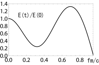
Figure 1: electric field decay with the production of the Nielsen-Olesen unstable modes.

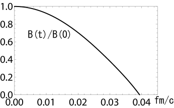
Figure 2: magnetic field decay with the production of the magnetic monopoles.

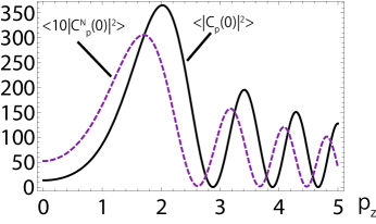
Figure 3: The initial amplitudes $\langle|C_{p}(t=0)|^{2}\rangle$ of the monopoles are 10 times larger than the initial amplitudes $\langle|C_{p}^{N}(t=0)|^{2}\rangle$ of Nielsen-Olesen unstable modes. The horizontal axis denotes momentum nomalized such as $p_{z}\equiv p/\sqrt{gB_{\rm{eff}}}$ for $\langle|C_{p}^{N}(t=0)|^{2}\rangle$ and $p_{z}\equiv p/\sqrt{g_{m}E_{\rm{eff}}}$ for $\langle|C_{p}(t=0)|^{2}\rangle$.

Here we make some comments on the magnetic ( $J_{m}$) and electric ( $J_{N}$ ) currents, for example, $J_{m}=\frac{2g_{m}k}{Ll_{\rm{E}}^{2}\pi}\int_{-\infty}^{+\infty}dp(p+g_{m}A_{\rm eff}^{d})|C_{p}|^{2}$ in eq(IV). The first comment is that $J_{m}$ vanishes at $t=0$ because $g_{m}A_{\rm eff}^{d}(t=0)=0$ and the integrand is antisymmetric in the variable $p$; $-p|C_{-p}(t=0)|^{2}=-p|C_{p}(t=0)|^{2}$. Similarly, the electric current $J_{N}$ vanishes at $t=0$. Then, the current begins to flow after the spontaneous production of the magnetic monopoles. The amount of the current is determined by the large amplitude of the monopole field $|C_{p}(t=0)|$ ( $\gg|C_{p}^{NO}(t=0)|$ ). This initial large amount of the monopole current causes the magnetic field decrease rapidly. The second one is concerned with the dependence of the currents on the parameter $k$. Because $J_{N}\propto k$ and $J_{m}\propto k$, the parameter $k$ can be absorbed by the amplitudes $C_{p}$ and $C_{p}^{N}$ in eq(IV) and eq(IV) with the replacement such as $C_{p}\to k^{-1/2}C_{p}$ and $C_{p}^{N}\to k^{-1/2}C_{p}^{N}$. Then, the equations of motion do not involve the parameter $k$. But, both of the initial amplitudes $C_{p}(t=0)$ and $C_{p}^{N}(t=0)$ acquire the factor $k^{1/2}$. Thus, the ratio of $|C_{p}(t=0)|^{2}$ to $|C_{p}^{N}(t=0)|^{2}$ is independent of $k$. This large value of the ratio $|C_{p}(t=0)|^{2}/|C_{p}^{N}(t=0)|^{2}\sim 10$ gives rise to the dominance of the monopole production in the glamsa decay. Therefore, although there is the ambiguity of the value $k$ used in our calculations, our result of the rapid glasma decay into the monopoles still holds. ( Here we have assumed that the rapid decay of the magnetic field into the monopoles also leads to the rapid decay of the electric field. This is because the flux tube of the electric field expandsinstability1 into the direction perpendicular to the tube, which generates magnetic field according to the dual Faraday’s law. Then the magnetic field may also decays into the monopoles. Thus, it turns out that the electric field also decays producing the magnetic monopoles. )

Our results have been obtained using the simplified initial conditions. The conditions are not proper ones. But using the initial conditions we obtain the same initial large amplitude as the one $\langle|C_{p}(t=0)|^{2}\rangle$ obtained by using the proper initial conditions. That is, Both initial conditions give rise to the large initial amplitudes of the monopole field, compared with the initial amplitudes of the Nielsen-Olesen unstable modes. As we have shown, these initial large amplitudes cause the rapid decay of the magnetic field. Hence, our conclusion of the rapid decay of the glasma into the monopoles may be reliable even if the simplified initial conditions are adopted.

V Discussions and Conclusions

We have shown that the glasma rapidly decays into magnetic monopoles. Then, it is natural to ask how the monopole gas leads to the thermalized QGP. Classical solutions of color magnetic monopoles are unstable unless their stability is guaranteed topologically. Indeed, there are no solutions of stable magnetic monopoles in real QCD. It has been showncoleman that the growth rates of unstable modes of gluons around classical monopoles can be infinitely large; the rates are proportional to the logarithm of the volume in the system. The fact indicates that the monopoles rapidly decay into gluons even if they are produced. Furthermore, they couple strongly with gluons because the smaller the $g$, the larger the coupling $g_{m}=2\pi/g$. Therefore, thermalized QGP would be generated immediately after the decay of the glasma into the monopoles.

In our analyses we have used a classical statistical field theory technique in order to take into account the one loop quantum effects of the monopoles and the unstable modes. To comfirm the validity of the technique, we need to clarify whether or not the higher order effects of these excitations change our results.

The model of the monopoles used in the present paper is a model of dual superconductor in which quark confinement is realized. The model is an effective model of the monopoles. It is not clear that the model is applicable to the analysis of the glasma decay. But, our results suggest that the monopoles play significant roles in the glasma decay. Therefore, it is desirable to perform more rigorous treatment of the monopoles in the analysis of the glasma.

The author expresses thanks to Prof. T. Kunihiro and Dr. N. Tanji for their useful comments.

References

- (1) E. Iancu, A. Leonidov and L. McLerran, hep-ph/0202270.
- (2) E. Iancu and R. Venugopalan, hep-ph/0303204.
- (3) T. Hirano and Y. Nara, Nucl. Phys. A743 (2004) 305; J. Phys. G30 (2004) S1139.
- (4) P. Romatschke and R. Venugopalan, Phys. Rev. Lett. 96 (2006) 062302; Phys. Rev. D74 (2006) 045011.
- (5) K. Fukushima and F. Gelis, Nucl. Phys. A874 (2012) 108.
- (6) J. Berges and S. Schlichting, Phys. Rev. D87 (2013) 014026.
- (7) J. Berges, S. Scheffler and D. Sexty, Phys. Rev. D77 (2008) 034504.
- (8) T. Kunihiro, B. Muller, A. Ohnishi, A. Schafer, T. T. Takahashi and A Yamamoto, Phys.Rev. D82 (2010) 114015.
- (9) H. Iida, T. Kunihiro, B. Muller, A. Ohnishi, A. Schafer and T. T. Takahashi, hep-ph/13041807.
- (10) N.K. Nielsen and P. Olesen, Nucl. Phys. B144 (1978) 376.
- (11) A. Iwazaki, Phys. Rev. C77 (2008) 034907; Prog. Theor. Phys. 121 (2009) 809.
- (12) H. Fujii and K. Itakura, Nucl. Phys. A809 (2008) 88.
- (13) H. Fujii, K. Itakura and A. Iwazaki, Nucl. Phys. A828 (2009) 178.
- (14) J. Berges, S. Scheffler, S. Schlichting and D. Sexty, Phys. Rev. D85 (2012) 034507.
- (15) S. Coleman, ”The magnetic monopole 50 years later” in The Unity of the Fundamental Interactions (1983), A. Zichichi, editor.
- (16) G.t’Hooft, High Energy Physics, edited by A. Zichichi ( Editorice Compositori, Bologna,1975 ).
- (17) S. Mandelstam, Phys. Rep 23 (1976) 245.
- (18) Z.F. Ezawa and A. Iwazaki, Phys. Rev. D25 (1982) 2681.
- (19) T. Suzuki and I. Yotsuyanagi, Phys. Rev. D42 (1990) 4257.
- (20) see a review article, G. Ripka, lecture notes in physics 639, Springer.
- (21) T. Suzuki and I. Yotsuyanagi, Phys. Rev. D42 (1990) 4257.
- (22) J.D. Stack, S.D. Neiman and R.J. Wensley, Phys. Rev. D50 (1994) 3399.
- (23) K. Amemiya and H. Suganuma, Phys. Rev. D60 (1999) 114509.
- (24) Y. Koma, M. Koma, E.-M. Ilgenfritz and T. Suzuki, Phys. Rev. D68, (2003) 114504.
- (25) K.I. Kondo, Phys. Lett. B600 (2004) 287.
- (26) J. Schwinger, Phys. Rev. 82 (1951) 664.
- (27) N. Tanji and K. Itakura, Phys. Lett. B173 (2012) 112.
- (28) K. Dusling, F. Gelis and R. Venugopalan, Nucl. Phys. A872 (2011) 161.
- (29) K. Dusling, T. Epelbaum, F. Gelis and R. Venugopalan, Phys. Rev. D86 (2012) 085040.
- (30) F. Gelis and N. Tanji, Phys. Rev. D87 (2013) 125035.
- (31) J. Liao and E. Shuryak, Phys. Rev. Lett. 101 (2008) 162302.
- (32) N. Tanji, Annals. Phys. 324 (2009) 1691 ( see the references therein ).
- (33) J. Berges, D. Gelfand, S. Scheffler and D. Sexty, Phys. Lett. B677 (2009) 210.
- (34) H.B. Nielsen and M. Ninomiya, Nucl. Phys. B156 (1979) 1.
- (35) A. Iwazaki, Phys. Rev. C87 (2013) 024903.