Hilfer fractional advection-diffusion equations with power-law initial condition; a Numerical study using variational iteration method

Abstract

We propose a Hilfer advection-diffusion equation of order $0<\alpha<1$ and type $0\leq\beta\leq 1$, and find the power series solution by using variational iteration method. Power series solutions are expressed in a form that is easy to implement numerically and in some particular cases, solutions are expressed in terms of Mittag-Leffler function. Absolute convergence of power series solutions is proved and the sensitivity of the solutions is discussed with respect to changes in the values of different parameters. For power law initial conditions it is shown that the Hilfer advection-diffusion PDE gives the same solutions as the Caputo and Riemann-Liouville advection-diffusion PDE. To leading order, the fractional solution compared to the non-fractional solution increases rapidly with $\alpha$ for $\alpha>0.7$ at a given time $t$; but for $\alpha<0.7$ this factor is weakly sensitive to $\alpha$. We also show that the truncation errors, arising when using the partial sum as approximate solutions, decay exponentially fast with the number of terms $n$ used. We find that for $\alpha<0.7$ the number of terms needed is weakly sensitive to the accuracy level and to the fractional order, $n\approx 20$; but for $\alpha>0.7$ the required number of terms increases rapidly with the accuracy level and also with the fractional order $\alpha$.

1 Introduction

Many transport phenomenon such as the time evolution of chemical or biological species in a flow field are often modeled by partial differential equations. These PDE’s are of the advection-diffusion-reaction type and can be derived from mass balance, momentum balance and energy balance equations and in the case of multi-component species, we also have individual species mass balance equations, see [1] and [2].

In a single-phase single-component system, let us denote the scalar concentration field by $c(x,t)$ at the position $x$ and at the time instant $t$, whose transport is described by the non-linear advection-diffusion-reaction equation,

$$\frac{\partial{c(x,t)}}{\partial{t}}+\frac{\partial}{\partial x}P(u(x,t),c(x,t))=-\frac{\partial}{\partial x}\left(J_{c}\right)+f(x,t,c(x,t)).$$ (1)

where $u(x,t)$ is the velocity field in which the scalar is transported, $P(u,c)$ is a non-linear convective flux, $J_{c}(x,t)$ is the scalar flux, and $f(x,t,c(x,t))$ is the source/reaction term. See Appendix A for details on how this eqaution is derived.

Many physical phenomena appearing in the studies of fluid mechanics, astrophysics, ground water flow, [12], meteorology, [13], [14], semiconductors, [7], and reactive flows, [15], are modeled by Eq. (1). The nonlinear advection-diffusion equation also proves to be effective in describing the behavior of two-phase flow in oil reservoir, [6], non-newtonian flows, [16], front propagation, [17], traffic flow, [18], financial modeling, [19].

Although the above mathematical models adequately describe a lot of natural phenomena, there still exist many complex phenomena in nature which are not described adequately by these models. Among them are crowded systems, such as protein diffusion within cells, [23], and diffusion through porous media, [24]. So there is a need to develop new models to understand such complex phenomena. In this regard fractional calculus could be helpful in describing such complex phenomena, see [25], [26], [27] and [28]. For instance, in order to obtain a better understanding of anomalous diffusion Caputo [29] used fractional calculus to incorporates memory.

Fractional calculus continues to attract the attention of researchers in physics, biology, chemistry and other engineering sciences [21]. The reason lies in its ability to explain the complex systems, such as, anomalous diffusion in porous media, crowding in living cells, time evolutionary processes which depend on the past history. Experimental evidence of anomalous diffusion have been reported by Hilfer [35] while working on dielectric spectroscopy (in particular, glassy formations and relaxations in polymers). Joen et al. [20] have reported their findings about the evidence of anomalous diffusion in living organism, and Tabie et al. [22], during the study of crowded systems (intra cellular transport of insulin in granules), have witnessed the anomalous diffusion of insulin in cells.

Anomalous diffusion, and transport through porous medium, can be understood as a random walk processes, [30], especially continuous time random walk (CTRW) models. Conventional, Brownian CTRW, is characterised by waiting times and jumps in particle location whose probability density function are Gaussian and the pdf obeys the classical advection-diffusion equation. Anomalous diffusion, on the other hand, possesses pdf’s of waiting times and jumps which are inverse power laws, and it can be shown that such a process is described by fractional advection-diffusion equations.

Furthermore, in a standard diffusion process the mean square displacement, MSD, $<x(t)^{2}>$ of a particle is linearly related to the time $t$, but in anomalous diffusion MSD $<x(t)^{2}>$ has a nonlinear power relationship with the time $t$, that is, $<x(t)^{2}>\propto t^{\alpha}$. For $0<\alpha<1$ diffusion is called subdiffusion; for $\alpha=1$, we have the standard diffusion; for $1<\alpha<2$ the diffusion is termed as superdiffusion. Mean square displacement can be understood geometrically as the amount of space the particle has explored in the system. For more details, see Metzler and Klafter [31]. They have obtained the following fractional advection-diffusion equation,

$$\frac{\partial}{\partial t}c(x,t)=\ _{0}\mathcal{D}^{1-\alpha}_{t}\left[K_{\alpha}\frac{\partial^{2}c(x,t)}{\partial x^{2}}-A_{\alpha}\frac{\partial}{\partial x}\left\{u(x)c(x,t)\right\}\right].$$ (2)

where $c(x,t)$ is a scalar field, ${}_{0}\mathcal{D}^{1-\alpha}_{t}$ is the Riemann-Liouville fractional derivative of order $0<\alpha<1$ defined in Eq. (5), $K_{\alpha}$ and $A_{\alpha}$ are called the generalized diffusion constants.

Note that Eq. (2) reduces to the problem considered by Caputo [29] by taking $A_{\alpha}=0$ and replacing $1-\alpha$ by $\alpha$ (using the same symbol). Also note that by setting $K_{\alpha}=1$, $A_{\alpha}=1$, and $\alpha=1/2$ in Eq. (2), we obtain a time fractional diffusion equation of order $1/2$ which was considered by Das in [32] and by Saha in [33].

In the present study, we propose a similar equation to (2) but with the Riemann-Liouville fractional derivative ${}_{0}\mathcal{D}^{1-\alpha}_{t}$ is replaced by the Hilfer fractional derivative ${}_{0}\mathcal{D}_{t}^{\alpha,\beta}$, (defined later in Eq. (8)). Hilfer fractional derivative ${}_{0}\mathcal{D}_{t}^{\alpha,\beta}$ is a sort of interpolation between the Riemann-Liouville fractional derivative and Caputo fractional derivative, see [34]. Example of a physical system that can be modeled by Hilfer fractional derivative is given by Hilfer in [35].

2 Problem statement: Hilfer fractional advection-diffusion system

We interpret $c(x,t)$ as a diffusive scalar field (for example temperature or concentration), and we use the simplifying assumption $K_{\alpha}=A_{\alpha}=\kappa=$constant in Eq. (2) and obtain the following linear fractional advection-diffusion equation,

$$\frac{\partial{c(x,t)}}{\partial{t}}=\kappa\ _{0}\mathcal{D}_{t}^{\alpha,\beta}\left[\frac{\partial^{2}c(x,t)}{\partial x^{2}}-\frac{\partial}{\partial x}\left\{u(x)c(x,t)\right\}\right],\quad x>0,t>0.$$ (3)

Equation (3) is called the Hilfer advection-diffusion equation of order $\alpha$ and type $\beta$; $\kappa>0$ represents diffusivity; $u(x)$ represents the velocity field. Note that equation (3) reduces to equation (2) by taking $\beta=0$ and relabeling $\alpha$ by $1-\alpha$. Also note that in [38] Sandev considers a diffusion-reaction equation that involves Hilfer fractional derivative but without the advection term.

Here we outline the main objectives of the present study. Firstly, we find the power series solution of Eq. (3), with $u(x)=-x$ and initial condition $c(x,0)=f(x)$ by using variational iteration method, described in Section (4). Secondly, we represent the power series solution in a convenient form that is easy to use for numerical purposes, especially we give a recurrence relation for the $x-$part in the $n$th term of the series. Thirdly, we prove the absolute convergence of the series solution accompanied by some examples. Fourthly, we analyze the behavior of the fractional solution with respect to the parameters $\alpha$, $\kappa$, and $p$; and we discuss the numerical convergence of the solutions which arise when we use the truncated series solution. Finally, we examine the fractional solutions for $\alpha>0$ and compare with the conventional solution for $\alpha=0$ in order to elucidate trends in the solution as $\alpha$ increases for different parameter values $p$ and $\kappa$.

We have organized this paper as follows: in Section 3, we provide some basic definitions and results from fractional calculus; in Section 4, we describe the variational iteration method to obtain the solution of the problem (3) subject to initial condition; in Section 5, we present a case study of polynomial uploading; in Section 6, we discuss the numerical results and provide graphs of the solutions along with error analysis; in Section 7, we compare the fractional solutions with the corresponding conventional versions; and in the last Section 8, we state our conclusions of the study.

3 Preliminaries

In this section, we briefly discuss the importance and significance of time fractional derivatives and Hilfer-composite time fractional derivative, and state some definitions and results from fractional calculus, see [38, 41].

It was shown by Hilfer that time fractional derivatives are equivalent to infinitesimal generators of generalized time fractional evolutions, which arise in the transition from microscopic to macroscopic time scales [35, 36]. Hilfer showed that this transition from ordinary time derivative to fractional time derivative indeed arises in physical problems [34, 37, 38, 40].

Riemann-Liouville Fractional Integral of order $\alpha$ for an absolutely integrable function $f(t)$ is defined by

$$\left({}_{0}I_{t}^{\alpha}f\right)(t):=\frac{1}{\Gamma(\alpha)}\int_{0}^{t}\frac{f(\tau)}{(t-\tau)^{1-\alpha}}d\tau,\quad t>0,\alpha>0$$ (4)

when the right hand side exists. Riemann-Liouville Fractional Derivative of order $\alpha>0$ for an absolutely integrable function $f(t)$ is defined by

$$\left({}_{0}D_{t}^{\alpha}f\right)(t)=\frac{1}{\Gamma(1-\alpha)}\frac{d}{dt}\int_{0}^{t}\frac{f(\tau)}{(t-\tau)^{\alpha}}d\tau,\qquad t>0,\quad 0<\alpha<1$$ (5)

Caputo Fractional Derivative of order $\alpha>0$ for a function $f(t)$, whose first derivative is absolutely integrable, is defined by

$$\left({}_{0}^{*}D_{t}^{\alpha}f\right)(t)=\frac{1}{\Gamma(1-\alpha)}\int_{0}^{t}\frac{f^{{}^{\prime}}(\tau)}{(t-\tau)^{\alpha}}d\tau,\qquad t>0,\quad 0<\alpha<1$$ (6)

Relationship between Riemann-Liouville and Caputo Fractional Derivative

$$\begin{aligned} \left({}_{0}^{*}D_{t}^{\alpha}f\right)(t)&=\ _{0}D_{t}^{\alpha}f(t)-f(0^{+})\frac{t^{-\alpha}}{\Gamma(1-\alpha)}\\ &=\ _{0}D_{t}^{\alpha}\left[f(t)-f(0^{+})\right].\end{aligned}$$ (7)

Hilfer Fractional Derivative of order $\alpha>0$ and type $\beta$ for an absolutely integrable function $f(t)$ with respect to $t$ is defined by,

$$\left({}_{0}D_{t}^{\alpha,\beta}f\right)(t)=\left({}_{0}I_{t}^{\beta(1-\alpha)}\frac{d}{dt}\ _{0}I_{t}^{(1-\beta)(1-\alpha)}f\right)(t),\qquad t>0,\quad 0<\alpha<1,0\leq\beta\leq 1.$$ (8)

Lemma 3.1.

[42] The following fractional derivative formula holds true:

$$_{0}D_{t}^{\alpha,\beta}\left(t^{\gamma}\right)=\frac{\Gamma(1+\gamma)}{\Gamma(1+\gamma-\alpha)}\left(t^{\gamma-\alpha}\right),\qquad t>0,\quad\gamma>-1,$$ (9)

where $0<\alpha<1$ and $0\leq\beta<1$.

From lemma 3.1, We can easily have the following lemma.

Lemma 3.2.

On integrating equation (9), we obtain

$$\int_{0}^{t}\ {}_{0}D_{t}^{\alpha,\beta}\left(t^{\gamma}\right)dt=\frac{\Gamma(1+\gamma)}{\Gamma(1-\alpha+\gamma+1)}\left(t^{1-\alpha+\gamma}\right),\qquad t>0,\quad\gamma>-1,$$ (10)

where $0<\alpha<1$ and $0\leq\beta<1$.

Remarks:

1. The Caputo derivative represents a type of regularization in the time domain (origin) for Riemann-Liouville derivative.

2. Hilfer fractional derivative interpolates between Riemann-Liouville fractional derivative and Caputo fractional derivative, because if $\beta=0$ then Hilfer fractional derivative corresponds to Riemann-Liouville fractional derivative and if $\beta=1$ then Hilfer fractional derivative corresponds to Caputo fractional derivative.

3. $f(0^{+})$ is required to be finite.

4. The three derivatives are equal if $f$ is continuous on $[0,T]$ and $f(0^{+})=0$, see Lemma 8.1.

Mittag-Leffler Function Mittag-Leffler function is the generalization of exponential function $e^{z}=\sum_{k=0}^{\infty}\frac{z^{k}}{k!}$. 1-parameter Mittag-Leffler Function

$$E_{\alpha}(z)=\sum_{k=0}^{\infty}\frac{z^{k}}{\Gamma(\alpha k+1)},\quad\alpha>0.$$ (11)

2-parameter Mittag-Leffler Function

$$E_{\alpha,\beta}(z)=\sum_{k=0}^{\infty}\frac{z^{k}}{\Gamma(\alpha k+\beta)},\quad\alpha>0,\beta>0.$$ (12)

The motivation of studying fractional equations of form (3) is, from one side, the Hilfer generalized time fractional derivative (8), which combine both the derivatives, Caputo and R–L. It is known, from the continuous time random walk (CTRW) theory, that the probability density $f(x,t)$, in case where the characteristic waiting time diverges and the jump length variance is finite, can be obtained from the following two equivalent representations of the fractional diffusion equation [39, 40]

$${}_{0}D_{t}^{\mu}f(x,t)-f(x,0^{+})\frac{t^{-\mu}}{\Gamma(1-\mu)}=\kappa\frac{\partial^{2}}{\partial x^{2}}f(x,t)$$

$${}_{0}^{*}D_{t+}^{\mu}f(x,t)=\kappa\frac{\partial^{2}}{\partial x^{2}}f(x,t)$$

in the R–L and Caputo sense, respectively, where $\kappa$ is the generalized diffusion constant of physical dimension $[\kappa]=m^{2}/s^{\mu}$, and $\mu$ is the anomalous diffusion exponent. Thus, if the initial conditions are properly taken into account, the Caputo and Riemann-liouville formulations of the time-fractional diffusion-advection equations are identical.

4 Variational Iteration Method

In this section, we describe the variational iteration method, [44], and provide an outline for its implementation. The VIM has been used extensively by several authors, see [45, 46, 47], in recent years to obtain series solutions of problems arising in different areas of applied mathematics and engineering. VIM has been successfully applied to solve problems like Riccati equation, heat equation, wave equation and many other problems. Ji-Huan He, [48, 49], proposed VIM to obtain the solutions of nonlinear differential equations. The method provides the solution in the form of a successive approximations that may converge to the exact solution if such a solution exists. In case where a closed form of the exact solution is not achievable, we use the truncated series, for instance, the $n$th partial sum of the series. VIM has certain advantages over the other proposed methods like Adomian decomposition method (ADM), [44], and homotopy perturbation method (HPM), see [47]. In the case of ADM a lot of work has to be done to compute the Adomian polynomials for nonlinear terms and in the case of HPM, a huge amount of calculation has to be done when degree of nonlinearity increases. On the other hand, no specific requirements are needed for nonlinear operators in order to use VIM. For instance, HPM requires an introduction of small parameter that is sometimes difficult to incorporate in the equation or its introduction may change the physics of the problem.

The basic concepts and main steps for the implementation of VIM are explained here. Consider the following equation:

$$\frac{\partial}{\partial t}c(x,t)=\ _{0}\mathcal{D}_{t}^{\alpha,\beta}[(Ac)(x,t)]+g(x,t),$$ (13)

where ${}_{0}\mathcal{D}_{t}^{\alpha,\beta}(.)$ represents the Hilfer fractional derivative with respect to time variable $t$, and $A$ represents a differential operator with respect to variable $x$.

The variational iteration method presents a correctional functional in $t$-direction for Eq. (13) in the form,

$$c_{n+1}(x,t)=c_{n}(x,t)+\int_{0}^{t}\lambda(\xi)\left(\frac{\partial{c_{n}(x,\xi)}}{\partial{\xi}}-\ _{0}\mathcal{D}_{t}^{\alpha,\beta}[A(\widetilde{c_{n}}(x,t))]-g(x,t)\right)d\xi,$$ (14)

with $c_{n}$ assumed known, where $\lambda(\xi)$ is a general Lagrange multiplier which can be identified optimally by variational theory and $\tilde{c}_{n}$ is a restricted value that means it behaves like a constant, hence $\delta\widetilde{c}_{n}=0$, where $\delta$ is the variational derivative.

The VIM is implemented in two basic steps, see [44];

1. the determination of the Lagrange multiplier $\lambda(\xi)$ that will be identified optimally through variational theory, and

2. with $\lambda(\xi)$ determined, we substitute the result into Eq. (14) where the restriction should be omitted.

Taking the $\delta-$variation of Eq. (14) with respect to $c_{n}$, we obtain

$$\delta c_{n+1}(x,t)=\delta c_{n}(x,t)+\delta\int_{0}^{t}\lambda(\xi)\left(\frac{\partial{c_{n}(x,\xi)}}{\partial{\xi}}-\ _{0}\mathcal{D}_{t}^{\alpha,\beta}[A(\widetilde{c_{n}}(x,t))]-g(x,t)\right)d\xi.$$ (15)

Since $\delta\widetilde{c_{n}}=0$ and $\delta g=0$, we have

$$\delta c_{n+1}(x,t)=\delta c_{n}(x,t)+\delta\int_{0}^{t}\lambda(\xi)\left(\frac{\partial{c_{n}(x,\xi)}}{\partial{\xi}}\right)d\xi.$$ (16)

To determine the Lagrange multiplier $\lambda(\xi)$, we integrate by parts the integral in Eq. (16), and noting that variational derivative of a constant is zero, that is, $\delta k=0$. Hence Eq. (16) yields

$$\delta c_{n+1}(x,t) =\delta c_{n}(x,t)+\delta c_{n}(x,\xi)\lambda(\xi)|_{\xi=t}-\int_{0}^{t}\frac{\partial}{\partial\xi}\lambda(\xi)\delta c_{n}(x,\xi)d\xi$$

$$=\delta c_{n}(x,t)(1+\lambda(\xi)|_{\xi=t})-\int_{0}^{t}\frac{\partial}{\partial\xi}\lambda(\xi)\delta c_{n}(x,\xi)d\xi$$ (17)

The extreme values of $c_{n+1}$ requires that $\delta c_{n+1}=0$. This means that left hand side of Eq. (4) is zero, and as a result the right hand side should be zero as well, that is,

$$\delta c_{n}(x,t)(1+\lambda(\xi)|_{\xi=t})-\int_{0}^{t}\frac{\partial}{\partial\xi}\lambda(\xi)\delta c_{n}(x,\xi)d\xi=0$$ (18)

This yields the stationary conditions

$$1+\lambda(\xi)|_{\xi=t}=0$$ (19)

$$\text{and }\lambda^{\prime}(\xi)=0$$ (20)

$$\text{which implies }\lambda=-1.$$ (21)

Hence Eq. (14) becomes

$$c_{n+1}(x,t)=c_{n}(x,t)-\int_{0}^{t}\left(\frac{\partial{c_{n}(x,\xi)}}{\partial{\xi}}-\ _{0}\mathcal{D}_{t}^{\alpha,\beta}[A(c_{n}(x,t))]-g(x,t)\right)d\xi,$$ (22)

where the restriction is removed on $c_{n}$. We can use Eq. (22) to obtain the successive approximation of the solution of the problem (13). The zeroth approximation $c_{0}(x,t)$ can be chosen in such away that it satisfies the initial condition and the boundary conditions. Appropriate selection of the zeroth approximation is necessary for the convergence of the successive approximation to the exact solution of the problem.

However, we remark that beacause VIM involves derivatives of all $c_{n}$’s inside the integral in the above equation, then VIM is limited to smooth initial conditions. It is not suitable for initial conditions such as $c_{0}(x)=\delta(x)$ – the latter would produce a Green’s function for the physical problem. Nevertheless, provided smooth initial conditions can be specified then VIM is often fast and very effective, as demonstrated in the case studies below.

4.1 Solution of the Problem

We consider the equation

$$\frac{\partial{c(x,t)}}{\partial{t}}=\kappa\ _{0}\mathcal{D}_{t}^{\alpha,\beta}\left[\frac{\partial^{2}c(x,t)}{\partial x^{2}}-\frac{\partial}{\partial x}\left\{u(x)c(x,t)\right\}\right],\quad x>0,t>0$$ (23)

with initial condition $c(x,0)=f(x).$

According to the variational iteration method, we consider the correctional functional in $t$-direction by using Eq. (14)

$$c_{n+1}(x,t)=c_{n}(x,t)+\int_{0}^{t}\lambda(\xi)\left(\frac{\partial{c_{n}(x,\xi)}}{\partial{\xi}}-\kappa\ _{0}\mathcal{D}_{\xi}^{\alpha,\beta}\left[\frac{\partial^{2}\widetilde{c}_{n}(x,\xi)}{\partial x^{2}}-\frac{\partial}{\partial x}\left\{u(x)\widetilde{c}_{n}(x,\xi)\right\}\right]\right)d\xi.$$ (24)

Now by using Eq. (22) we obtain

$$c_{n+1}(x,t)=c_{n}(x,t)-\int_{0}^{t}\left(\frac{\partial{c_{n}(x,\xi)}}{\partial{\xi}}-\kappa\ _{0}\mathcal{D}_{\xi}^{\alpha,\beta}\left[\frac{\partial^{2}c_{n}(x,\xi)}{\partial x^{2}}-\frac{\partial}{\partial x}\left\{u(x)c_{n}(x,\xi)\right\}\right]\right)d\xi.$$ (25)

which simplifies to

$$c_{n+1}(x,t)=c_{n}(x,0)+\kappa\int_{0}^{t}\ {}_{0}\mathcal{D}_{\xi}^{\alpha,\beta}\left[\frac{\partial^{2}c_{n}(x,\xi)}{\partial x^{2}}-\frac{\partial}{\partial x}\left\{u(x)c_{n}(x,\xi)\right\}\right]d\xi.$$ (26)

Starting with an initial approximation $c_{0}(x,t)=c(x,0)=f(x)$, we obtain a sequence of successive approximations, and the exact solution is obtained by taking the limit of the $n$th approximation, that is,

$$c(x,t)=\lim_{n\rightarrow\infty}c_{n}(x,t).$$ (27)

5 A Case Study

5.1 Polynomial Uploading

We take $u(x)=-x$ in Eq. (23), so it becomes

$$\frac{\partial{c(x,t)}}{\partial{t}}=\kappa\ _{0}\mathcal{D}_{t}^{\alpha,\beta}\left[\frac{\partial^{2}c(x,t)}{\partial x^{2}}+\frac{\partial}{\partial x}\left\{xc(x,t)\right\}\right],\quad x>0,t>0$$ (28)

with the initial condition $c(x,0)=x^{p}$, for $p\geq 0$. We obtain the following iteration formula by using Eq. (25)

$$c_{n+1}(x,t)=c_{n}(x,0)+\kappa\int_{0}^{t}\ {}_{0}\mathcal{D}_{\xi}^{\alpha,\beta}\left[\frac{\partial^{2}c_{n}(x,\xi)}{\partial x^{2}}+\frac{\partial}{\partial x}\left\{xc_{n}(x,\xi)\right\}\right]d\xi,$$ (29)

with the zeroth approximation

$$c_{0}(x,t)=x^{p}.$$ (30)

By taking $n=0$ in Eq. (29) and using Eq. (30), we obtain

$$c_{1}(x,t)=x^{p}+\kappa\int_{0}^{t}\ {}_{0}\mathcal{D}_{\xi}^{\alpha,\beta}\left[\frac{\partial^{2}}{\partial x^{2}}x^{p}+\frac{\partial}{\partial x}\left\{x^{p+1}\right\}\right]d\xi,$$ (31)

which can be written as

$$c_{1}(x,t)=x^{p}+\kappa a_{1}(x)\int_{0}^{t}\ {}_{0}\mathcal{D}_{\xi}^{\alpha,\beta}(1)d\xi,$$ (32)

where

$$a_{1}(x)=\frac{\partial^{2}}{\partial x^{2}}x^{p}+\frac{\partial}{\partial x}\left\{x^{p+1}\right\}.$$ (33)

By using Lemma 3.1 and 3.2, we obtain

$$c_{1}(x,t)=x^{p}+\kappa a_{1}(x)\frac{t^{1-\alpha}}{\Gamma(1-\alpha+1)}.$$ (34)

Importantly, note that for the functions of type $f(t)=t^{\nu}$, where $\nu>-1$, the Hilfer fractional derivative is independent of $\beta$ by Lemma 3.1. Moreover, for such functions, the Caputo, Reimann-Liouville and Hilfer derivatives are all equal.

Furthermore, because this is the first term in the recurrence relation, $\beta$ does not appear in any of the higher order terms (below).

By taking $n=1$ in Eq. (29) and using Eq. (34), we obtain

$$c_{2}(x,t)=x^{p}+\kappa a_{1}(x)\frac{t^{1-\alpha}}{\Gamma(1-\alpha+1)}+\kappa^{2}a_{2}(x)\frac{t^{2(1-\alpha)}}{\Gamma(2(1-\alpha)+1)},$$ (35)

where

$$a_{2}(x)=\frac{\partial^{2}}{\partial x^{2}}a_{1}(x)+\frac{\partial}{\partial x}\left\{xa_{1}(x)\right\}.$$ (36)

By taking $n=2$ in Eq. (29) and using Eq. (35), we obtain

$$c_{3}(x,t)=x^{p}+\kappa a_{1}(x)\frac{t^{1-\alpha}}{\Gamma(1-\alpha+1)}+\kappa^{2}a_{2}(x)\frac{t^{2(1-\alpha)}}{\Gamma(2(1-\alpha)+1)}+\kappa^{3}a_{3}(x)\frac{t^{3(1-\alpha)}}{\Gamma(3(1-\alpha)+1)},$$ (37)

where

$$a_{3}(x)=\frac{\partial^{2}}{\partial x^{2}}a_{2}(x)+\frac{\partial}{\partial x}\left\{xa_{2}(x)\right\}.$$ (38)

Proceeding in this way we obtain

$$c_{n}(x,t)=x^{p}+\Sigma_{k=1}^{n}\kappa^{k}a_{k}(x)\frac{t^{k(1-\alpha)}}{\Gamma(k(1-\alpha)+1)},$$ (39)

where

$$a_{k}(x)=\frac{\partial^{2}}{\partial x^{2}}a_{k-1}(x)+\frac{\partial}{\partial x}\left\{xa_{k-1}(x)\right\},$$ (40)

and $a_{1}(x)$ is given by the Eq. (33). By setting $a_{0}(x)=x^{p}$, Eq. (39) can be written as

$$c_{n}(x,t)=\Sigma_{k=0}^{n}a_{k}(x)\frac{\kappa^{k}t^{k(1-\alpha)}}{\Gamma(k(1-\alpha)+1)}.$$ (41)

By taking the limit $n\rightarrow\infty$ of Eq. (41) we obtain

$$c(x,t)=\lim_{n\rightarrow\infty}c_{n}(x,t)=\Sigma_{k=0}^{\infty}a_{k}(x)\frac{\kappa^{k}t^{k(1-\alpha)}}{\Gamma[k(1-\alpha)+1]}.$$ (42)

We remark, again, that the final solution above does not contain any dependency on $\beta$. This is a consequence of the Lemma 3.1.

5.2 On the Convergence of $c(x,t)$

Theorem 5.1.

The series solution (42) of the problem (28) with the initial condition $c(x,0)=x^{p}$, $p\geq 0$, converges absolutely for all $x$ and $t$.

Proof.

We denote the $n$th term of Eq. (42) by

$$s_{n}(x,t)=a_{n}(x)\frac{\kappa^{n}t^{n(1-\alpha)}}{\Gamma[n(1-\alpha)+1]}.$$

Applying the ratio test on the series (42), we obtain

$$\left|\frac{s_{n+1}(x,t)}{s_{n}(x,t)}\right| =\left|\frac{a_{n+1}(x)}{a_{n}(x)}\kappa t^{(1-\alpha)}\frac{\Gamma[n(1-\alpha)+1]}{\Gamma[(n+1)(1-\alpha)+1]}\right|$$

$$\text{since }(1-\alpha)>0\text{ therefore }n(1-\alpha)+1>1$$

$$=\left|\frac{a_{n+1}(x)}{a_{n}(x)}\kappa t^{(1-\alpha)}\right|\frac{\Gamma[n(1-\alpha)+1]}{\Gamma[(n+1)(1-\alpha)+1]}.$$ (43)

Note that $\left|\frac{a_{n+1}(x)}{a_{n}(x)}\right|$ is bounded above by $p+1$, where $p\geq 0$ is the integer power of $x$ in the initial condition $c(x,0)=x^{p}$. Indeed, $a_{n}(x)$, defined in Eq. (40), is a polynomial in $x$ whose leading term, that is, the term with the highest power of $x$ is $(p+1)^{n}x^{p}$, and further note that degree$(a_{n}(x))=p$ for all $n\geq 0$. Thus we can approximate $a_{n}(x)$ by its leading term $(p+1)^{n}x^{p}$ (since all the coefficients are positive) and therefore we obtain

$$\left|\frac{a_{n+1}(x)}{a_{n}(x)}\right|\approx\left|\frac{(p+1)^{n+1}x^{p}}{(p+1)^{n}x^{p}}\right|=p+1.$$

By using Wendel’s double inequality, see [50],

$$x^{1-s}\leq\frac{\Gamma(x+1)}{\Gamma(x+s)}\leq(x+s)^{1-s},$$

for $x>0$ and $0<s<1$, we deduce that

$$\lim_{n\rightarrow\infty}\frac{\Gamma[n(1-\alpha)+1]}{\Gamma[(n+1)(1-\alpha)+1]}=0.$$

Hence, Eq. (5.2) gives

$$\lim_{n\rightarrow\infty}\left|\frac{s_{n+1}(x,t)}{s_{n}(x,t)}\right|=0.$$ (44)

Thus the series solution obtained in Eq. (42) converges (absolutely) for all $x$ and $t$ and for all real $p$. ∎

5.3 To show that $c(x,t)$ obtained in Eq. (42) satisfies Eq. (28)

Theorem 5.2.

The series solution (42) satisfies the equation (28) with the initial condition $c(x,0)=x^{p}$, where $p\geq 0$.

Proof.

First, on differentiating Eq. (42) with respect to $t$, we obtain

$$\frac{\partial}{\partial t}c(x,t) =\frac{\partial}{\partial t}\left[a_{0}(x)+\Sigma_{k=1}^{\infty}a_{k}(x)\frac{\kappa^{k}t^{k(1-\alpha)}}{\Gamma[k(1-\alpha)+1]}\right]$$

$$=\Sigma_{k=1}^{\infty}a_{k}(x)\frac{\kappa^{k}}{\Gamma[k(1-\alpha)+1]}\frac{\partial}{\partial t}t^{k(1-\alpha)}$$

$$=\Sigma_{k=1}^{\infty}a_{k}(x)\frac{\kappa^{k}}{k(1-\alpha)\Gamma[k(1-\alpha)]}k(1-\alpha)t^{k(1-\alpha)-1}$$

$$=\Sigma_{k=1}^{\infty}a_{k}(x)\frac{\kappa^{k}t^{k(1-\alpha)-1}}{\Gamma[k(1-\alpha)]}.$$ (45)

On the other hand substituting Eq. (42) in the right hand side of Eq. (28) yields

$$\kappa\ _{0}\mathcal{D}_{t}^{\alpha,\beta}\left[\frac{\partial^{2}c(x,t)}{\partial x^{2}}+\frac{\partial}{\partial x}\left\{xc(x,t)\right\}\right]$$

$$=\kappa\ _{0}\mathcal{D}_{t}^{\alpha,\beta}\left[\Sigma_{k=0}^{\infty}\left\{\frac{\partial^{2}}{\partial x^{2}}a_{k}(x)+\frac{\partial}{\partial x}x^{q}a_{k}(x)\right\}\frac{\kappa^{k}t^{k(1-\alpha)}}{\Gamma[k(1-\alpha)+1]}\right]$$

$$=\kappa\Sigma_{k=0}^{\infty}\left\{\frac{\partial^{2}}{\partial x^{2}}a_{k}(x)+\frac{\partial}{\partial x}x^{q}a_{k}(x)\right\}\ _{0}\mathcal{D}_{t}^{\alpha,\beta}\frac{\kappa^{k}t^{k(1-\alpha)}}{\Gamma[k(1-\alpha)+1]}$$

$$=\Sigma_{k=0}^{\infty}a_{k+1}(x)\frac{\kappa^{k+1}t^{(k+1)(1-\alpha)-1}}{\Gamma[(k+1)(1-\alpha)]}$$

$$=\Sigma_{k=1}^{\infty}a_{k}(x)\frac{\kappa^{k}t^{k(1-\alpha)-1}}{\Gamma[k(1-\alpha)]}.$$ (46)

The equality of Eqs. (5.3) and (5.3) proves that $u(x,t)$ given by Eq. (42) is the solution of problem (28). ∎

5.4 Examples

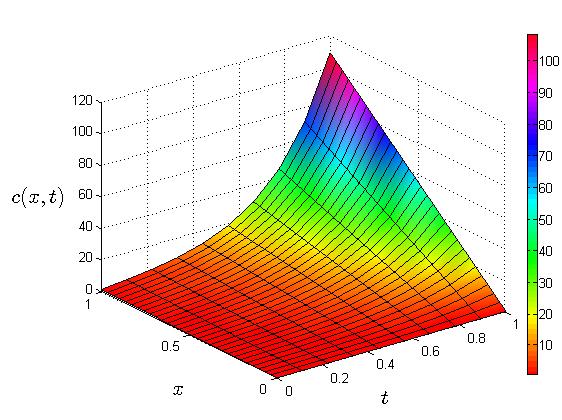
Figure 1: Plot of the solution $c(x,t)$, Eq. (47) (Example 1), for $0\leq x\leq 1$ and time $0<t<1$, where $p=1$, $\alpha=0.5$ and $\kappa=1$.

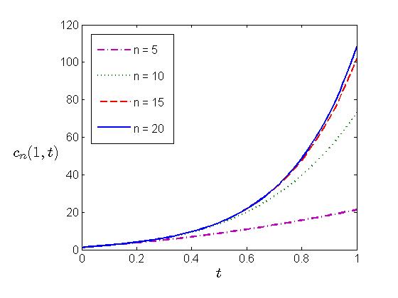
Figure 2: Plots of the truncated series solution $c_{n}(x,t)$, Eq. (48), (Example 1) for $0<t<1$ at $x=1$, where $p=1$, $\alpha=0.5$ and $\kappa=1$, for different $n$ as indicated.

We examine the solutions for the cases $p=1$ and $2$.

For $p=1$, the initial condition becomes $c(x,0)=x$, in Eq. (28). Then $a_{k}(x)=2^{k}x$ for $k\geq 0$ and hence from Eq. (42) the solution $c(x,t)$ is expressed as follows

$$c(x,t)=x\Sigma_{k=0}^{\infty}\frac{[2\kappa t^{1-\alpha}]^{k}}{\Gamma[k(1-\alpha)+1]}=xE_{1-\alpha}[2\kappa t^{1-\alpha}],$$ (47)

where $E_{\alpha}(t)$, defined in Eq. (11), is the Mittag-Leffler function in one parameter. The plot of the solution (47) is shown in the Fig. 2 for the values $\alpha=0.5$ and $\kappa=1$. Note that the solution $c(x,t)$, for fixed $t$, increases linearly with respect to variable $x$ and it increases exponentially with respect to variable $t$, for fixed $x$. In order to see, how rapidly the sequence of successive approximations provided by VIM converges to the exact solution, we use the $n$th partial sum as an approximation,

$$c_{n}(x,t)=x\Sigma_{k=0}^{n}\frac{[2\kappa t^{1-\alpha}]^{k}}{\Gamma[k(1-\alpha)+1]},$$ (48)

In Fig. 2, we plot $c_{n}(x,t)$ against $t$ at $x=1$ for $\alpha=0.5$ and $\kappa=1$, for different values of $n$. One can see from Fig. 2 that the solution converges by $n=20$. Later in Section 6, we will provide details about how many terms have to be summed up in order to obtain a given accuracy.

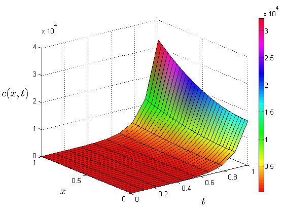
Figure 3: Plot of the solution $c(x,t)$, Eq. (49) (Example 2), for $0\leq x\leq 1$ and time $0<t<1$, where $p=2$, $\alpha=0.5$ and $\kappa=1$.

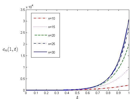
Figure 4: Plots of the truncated series solution $c_{n}(x,t)$, Eq. (5.4), (Example 2), for $0<t<1$ at $x=1$, where $p=2$, $\alpha=0.5$ and $\kappa=1$, for different $n$ as indicated.

For $p=2$ the initial condition becomes $c(x,0)=x^{2}$, in Eq. (28). Then $a_{k}(x)=3^{k}x^{2}+3^{k}-1$ for $k\geq 0$ and hence from Eq. (42) the solution $c(x,t)$ is expressed as follows

$$c(x,t)=x^{2}E_{1-\alpha}[3\kappa t^{1-\alpha}]+E_{1-\alpha}[3\kappa t^{1-\alpha}]-E_{1-\alpha}[\kappa t^{1-\alpha}].$$ (49)

The plot of the solution (49) is shown in the Fig. 4 for $\alpha=0.5$ and $\kappa=1$. This time, the solution $c(x,t)$, for fixed $t$, increases quadratically with respect to variable $x$ and it increases exponentially with respect to variable $t$, for fixed $x$.

Again, we use the $n$th approximation in order to see how rapidly the sequence of successive approximations provided by VIM converges to the exact solution:

$$c_{n}(x,t) =x^{2}\Sigma_{k=0}^{n}\frac{[3\kappa t^{1-\alpha}]^{k}}{\Gamma[k(1-\alpha)+1]}+\Sigma_{k=0}^{n}\frac{[3\kappa t^{1-\alpha}]^{k}}{\Gamma[k(1-\alpha)+1]}$$

$$\quad-\Sigma_{k=0}^{n}\frac{[\kappa t^{1-\alpha}]^{k}}{\Gamma[k(1-\alpha)+1]},$$ (50)

and plot it for different values of $n$. Figure 4 shows the plots of $c_{n}(x,t)$ against $t$ for $x=1$, $\alpha=0.5$, $\kappa=1$, and for different $n$ as indicated. This time the approximate solutions converge at $n=25$.

When $p\geq 3$, closed form solutions for $c(x,t)$ becomes increasingly harder to obtain. Nevertheless, for the purposes of analyzing the behavior of the solution $c(x,t)$ we require only the dominant term in the solution. As mentioned in Section 5.2 that we can approximate $a_{n}(x)$ by its leading term, that is by $(p+1)^{n}x^{p}$. If we replace $a_{n}(x)$ by $(p+1)^{n}x^{p}$ in Eq. (42), we obtain the the leading term to be,

$$c(x,t) \approx\Sigma_{k=0}^{\infty}(p+1)^{n}x^{p}\frac{\kappa^{k}t^{k(1-\alpha)}}{\Gamma[k(1-\alpha)+1]}$$

$$\approx x^{p}\Sigma_{k=0}^{\infty}\frac{[(p+1)\kappa t^{1-\alpha}]^{k}}{\Gamma[k(1-\alpha)+1]}$$

$$\approx x^{p}E_{1-\alpha}[(p+1)\kappa t^{1-\alpha}].$$ (51)

The solution $c(x,t)$ is thus proportional to $x^{p}$ at fixed t; and it increases approximately exponentially with respect to variable $t$ at fixed $x$.

In order to further investigate the trends in the fractional solution, we compare the fractional solution to the non-fractional solution at $x=1$ and $t=1$.

At $x=1$ and $t=1$, we get $c(1,1)\approx E_{1-\alpha}[(p+1)\kappa]$, and by using Eq. (11) we obtain

$$c(1,1)\approx\sum_{k=0}^{\infty}\frac{[(p+1)\kappa]^{k}}{\Gamma[k(1-\alpha)+1]}.$$

In the asymptotic limit $\alpha\rightarrow 1$, we obtain $c(1,1)\approx\sum_{k=0}^{\infty}[(p+1)\kappa]^{k}$, which is a geometric series and it converges to $\frac{1}{1-(p+1)\kappa}$, when $(p+1)\kappa<1$ or $\kappa<\frac{1}{p+1}$.

For $\alpha=0$, we obtain

$$c(1,1)\approx\sum_{k=0}^{\infty}\frac{[(p+1)\kappa]^{k}}{k!}$$

which converges for all $\kappa$ and $p\geq 0$.

Furthermore, in Eq. (5.4) in the asymptotic limit $\alpha\rightarrow 1$, $t^{1-\alpha}=1$ for all $t$, and thus the power series (5.4) converges for all $t$ so long as $(p+1)\kappa<1$.

6 Numerical Analysis and behavior of the solution

In this section we discuss the general behavior of the solution of the problem (28) with respect to different parameters and also we do some numerical analysis of the solution.

6.1 Reciprocal Gamma Function

First we analyze the reciprocal gamma function which appears in the series solution (42), that is,

$$\frac{1}{\Gamma[n(1-\alpha)+1]}.$$

The limit of this function, for a fixed $\alpha(\neq 1)$, as $n\to\infty$ is zero, that is,

$$\lim_{n\to\infty}\frac{1}{\Gamma[n(1-\alpha)+1]}=0,\quad\text{ for fixed }\alpha\in(0,1).$$

We want an expression for the number of terms $n$ needed in order to satisfy a given accuracy given by,

$$\frac{1}{\Gamma[n(1-\alpha)+1]}\leq 10^{-\tau},$$

for a given $\alpha$ and tolerance level $\tau$. For this purpose, we use the following formula, see [51],

$$\sqrt{2\pi x}(x/e)^{x}(x\sinh 1/x)^{x/2}(1+a/x^{5})<\Gamma(x+1)$$

$$<\sqrt{2\pi x}(x/e)^{x}(x\sinh 1/x)^{x/2}(1+b/x^{5}),$$

for all $x>0$ and with the optimal constants $a=0$ and $b=\frac{1}{1620}$, to obtain the required $n$. Table 1 summarizes this information.

Figure 6 shows the plots of $n$ against $\tau$ for different values of $\alpha$. For any given $\alpha$ the number of terms $n$ appears to scale almost linearly with $\tau$. Best linear fits were therefore obtained; for example for $\alpha=0.9$, we obtain the best fit $n=40.79+8.964\tau$. The graph of this linear equation is the solid line shown in the Fig. 6 along with the $95\%$ prediction intervals, whereas the simulation data are plotted as the symbols. The value of $R^{2}$, the coefficient of determination, is $99.8\%$ represents the percent of observed variability explained by the linear model, whereas the value of $R_{adj}^{2}$ is $99.7\%$ which is a more realistic quantity as it accounts for the number of terms in the model.

$\tau$	$\alpha$
	$0$	$0.1$	$0.2$	$0.3$	$0.4$	$0.5$	$0.6$	$0.7$	$0.8$	$0.9$
$4$	$8$	$9$	$10$	$11$	$13$	$15$	$19$	$25$	$37$	$74$
$6$	$10$	$11$	$12$	$14$	$16$	$19$	$24$	$32$	$48$	$95$
$8$	$12$	$13$	$15$	$17$	$19$	$23$	$29$	$38$	$57$	$114$
$10$	$14$	$15$	$17$	$19$	$22$	$27$	$33$	$44$	$66$	$132$
$12$	$15$	$17$	$19$	$22$	$25$	$30$	$38$	$50$	$75$	$150$
$14$	$17$	$19$	$21$	$24$	$28$	$34$	$42$	$56$	$83$	$166$
$16$	$19$	$21$	$23$	$26$	$31$	$37$	$46$	$61$	$91$	$182$

Table 1: The number of terms, $n$, needed to achieve a given tolerance level $10^{-\tau}$ for different $\alpha$.

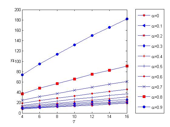
Figure 5: Plots of $n$ against $\tau$, for specific values of $\alpha$

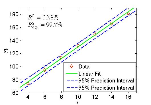
Figure 6: A linear relationship is observed between $\tau$ and $n$. Here, $\alpha=0.9$.

Figure 8 shows the plots of $n$ against $\alpha$ for some tolerance levels, taken from the data in Table 1. The relationship between $n$ and $\alpha$ is clearly non-linear.

For $\alpha\in(0,0.7)$ the number of terms needed for a given tolerance level $10^{-\tau}$ remains approximately constant; in fact even for different tolerance levels $n$ appears to be approximately insensitive to $\alpha$ and to $\tau$ – as a rule of thumb we see that $n\approx 20$ for $\alpha<0.7$.

But for $\alpha>0.7$ we see a rapid increase in the number of terms $n$ needed to achieve a given accuracy. It may be possible to find best-fit curves to the data plotted in Fig. 8. For this purpose, we assume cubic polynomial fits of the form $n(\alpha)=A+B\alpha+C\alpha^{2}+D\alpha^{3}$, where $A,B,C$ and $D$ are constants to be determined from the data using the least square method, for a tolerance level of $10^{-16}$, we obtain the following cubic polynomial $n(\alpha)=13.69+181.3\alpha-665.6\alpha^{2}+730.4\alpha^{3}$. The graph of this cubic polynomial is the solid line shown in the Fig. 8 along with the $95\%$ prediction interval, whereas the simulation data are plotted symbols. The value of $R^{2}$, is $97.5\%$, and $R_{adj}^{2}$ is $96.2\%$.

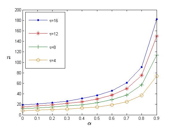
Figure 7: Plots of $n$ against $\alpha$, for specific tolerance levels $10^{-\tau}$.

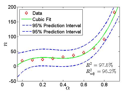
Figure 8: A cubic relationship is observed between $\alpha$ and $n$. Here, the tolerance level is $10^{-16}$.

$p$	$\kappa$	$\alpha$
		$0$	$0.1$	$0.2$	$0.3$	$0.4$	$0.5$	$0.6$	$0.7$	$0.8$	$0.9$
1	$0.1$	$1.2214$	$1.2339$	$1.2456$	$1.2563$	$1.2655$	$1.2726$	$1.2769$	$1.2777$	$1.2740$	$1.2650$
	$0.2$	$1.4918$	$1.5288$	$1.5666$	$1.6046$	$1.6417$	$1.6762$	$1.7056$	$1.7257$	$1.7311$	$1.7140$
	$0.3$	$1.8221$	$1.9018$	$1.9891$	$2.0845$	$2.1881$	$2.2989$	$2.4132$	$2.5225$	$2.6064$	$2.6228$
	$0.4$	$2.2255$	$2.3745$	$2.5486$	$2.7548$	$3.0024$	$3.3039$	$3.6758$	$4.1366$	$4.6886$	$5.2181$
	$0.5$	$2.7183$	$2.9749$	$3.2946$	$3.7041$	$4.2486$	$5.0090$	$6.1471$	$8.0407$	$11.8230$	$23.1605$
	$0.6$	$3.3201$	$3.7394$	$4.2952$	$5.0672$	$6.2094$	$8.0628$	$11.5427$	$20.0518$	$58.6544$	$916.0995$
2	$0.1$	$1.5945$	$1.6353$	$1.6758$	$1.7151$	$1.7518$	$1.7839$	$1.8084$	$1.8219$	$1.8194$	$1.7957$
	$0.2$	$2.4228$	$2.5697$	$2.7325$	$2.9127$	$3.1107$	$3.3251$	$3.5495$	$3.7672$	$3.9389$	$3.9806$
	$0.3$	$3.5693$	$3.9406$	$4.3938$	$4.9582$	$5.6782$	$6.6248$	$7.9175$	$9.7701$	$12.5841$	$16.9670$
	$0.33$	$3.9915$	$4.4651$	$5.0595$	$5.8263$	$6.8503$	$8.2856$	$10.4192$	$13.9340$	$20.7619$	$39.3061$
	$0.4$	$5.1418$	$5.9195$	$7.0055$	$8.5392$	$10.7960$	$14.4464$	$21.3697$	$38.3904$	$115.8880$	$9036.86$
3	$0.1$	$2.3031$	$2.4136$	$2.5300$	$2.6500$	$2.7704$	$2.8871$	$2.9914$	$3.0700$	$3.1023$	$3.0610$
	$0.15$	$3.2389$	$3.4888$	$3.7704$	$4.0874$	$4.4422$	$4.8342$	$5.2536$	$5.6714$	$6.0144$	$6.1219$
	$0.2$	$4.4267$	$4.9114$	$5.4945$	$6.2053$	$7.0842$	$8.1867$	$9.5866$	$11.3700$	$13.5612$	$15.7306$
	$0.25$	$5.9270$	$6.7868$	$7.8886$	$9.3416$	$11.3284$	$14.1788$	$18.5512$	$25.9800$	$41.0229$	$86.4111$
	$0.3$	$7.8141$	$9.2522$	$11.2138$	$14.0152$	$18.2732$	$25.3548$	$38.9312$	$72.6400$	$227.4317$	$18069.2957$
4	$0.10$	$3.6044$	$3.9008$	$4.2330$	$4.6032$	$5.0110$	$5.4495$	$5.8996$	$6.3177$	$6.6170$	$6.6440$
	$0.14$	$5.3248$	$5.9671$	$6.7391$	$7.6743$	$8.8142$	$10.2060$	$11.8918$	$13.8682$	$15.9573$	$17.4156$
	$0.18$	$7.5956$	$8.8247$	$10.4021$	$12.4722$	$15.2609$	$19.1376$	$24.7363$	$33.2074$	$46.7204$	$68.5890$
	$0.20$	$8.9816$	$10.6300$	$12.8138$	$15.7965$	$20.0255$	$26.3213$	$36.3427$	$53.9703$	$90.7746$	$203.926$
	$0.22$	$10.5624$	$12.7377$	$15.7134$	$19.9434$	$26.2635$	$36.7332$	$54.2600$	$91.6757$	$202.0610$	$1272.2308$

Table 2: The solution $c(1,1)$ for different parameter values $p$, $\alpha$ and $\kappa$.

6.2 Behavior of the Solution

The solution of the problem (28) (with $u(x)=-x$, and initial condition $c(x,0)=x^{p}$, $p>0$) is given by

$$c(x,t)=\Sigma_{n=0}^{\infty}a_{n}(x)\frac{(\kappa t^{1-\alpha})^{n}}{\Gamma[n(1-\alpha)+1]},$$

where

$$a_{n}(x)=\frac{\partial^{2}}{\partial x^{2}}a_{n-1}(x)+\frac{\partial}{\partial x}\left\{xa_{n-1}(x)\right\},$$

and $a_{0}(x)=x^{p}$.

We now examine the sensitivity of the solution $c(x,t)$ to parameters $p$, $\kappa$ the diffusivity coefficient, and to $\alpha$ the order of the Hilfer derivative. We choose the following values: $p\in\{1,2,3,4\}$, $\alpha\in\{0,0.1,...,0.9\}$ and we select $\kappa$ according to $\kappa<\frac{1}{p+1}$. We compare the values of $c(x,t)$ at the point $(1,1)$ for different combinations of the above parameters. We choose three values of $\kappa$ that are less than $\frac{1}{p+1}$ and one value that is equal (approximately) to $\frac{1}{p+1}$ and one value that is greater than $\frac{1}{p+1}$. The data is collected in Table 2 and it reveals that different combinations of parameter’s values affect the values of $c(x,t)$ differently. In general, we note that an increase in the values of parameters $p$, $\kappa$ and $\alpha$ results into an increase in the values of $c(x,t)$. The effect of $\kappa$ can be divided into two parts, first when $\kappa<\frac{1}{p+1}$ and second when $\kappa\geq\frac{1}{p+1}$.

For the first case, $\kappa<\frac{1}{p+1}$, the increase in the values of $c(x,t)$ is not significant as compare to the second case, $\kappa\geq\frac{1}{p+1}$, where $c(x,t)$ increases very rapidly with $\alpha$ and $\kappa$.

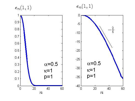
Figure 9: Plot of the relative error $e_{n}(1,1)$ against the number of terms $n$, from example 1. Left: Linear-Linear, Right: Linear-Natural Log (y-axis is scaled as $e^{m}$, where $m\in\{-40,-35,\dots,0\}$). A line of slope $-2/5$ is shown for comparison.

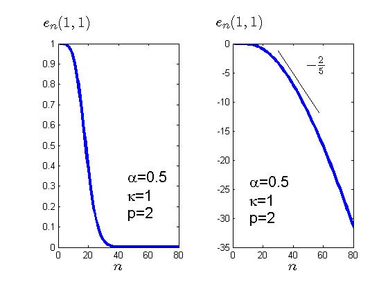
Figure 10: Plot of the relative error $e_{n}(1,1)$ against the number of terms $n$, from example 2. Left: Linear-Linear, Right: Linear-Natural Log (y-axis is scaled as $e^{m}$, where $m\in\{-35,-30,\dots,0\}$). A line of slope $-2/5$ is shown for comparison.

6.3 Relative Error

Finally, we examine the truncation error when using the partial sum of first $n$ terms of the series solution given in Eq. (42). We define the relative error as,

$$e_{n}(x,t)=\frac{|c(x,t)-c_{n}(x,t)|}{|c(x,t)|},$$

where $c_{n}(x,t)$ is the partial sum of the first $n$ terms. Figures 10 and 10 show the plots of $e_{n}(x,t)$ versus $n$ at the point $(1,1)$ for, respectively, $p=1$ (Example 1), and $p=2$ (Example 2). The errors fall off exponentially fast with $n$, $e_{n}\approx\exp(-2/5)$.

It is not always possible to express the series solution in compact form like in the cases of $p=1$ and $p=2$. For values of $p$ larger than $2$, we approximate the ’exact’ solution by taking a very large value of $n$, and then we compare this with the smaller values of $n$. For example, when the initial condition is $f(x)=x^{3}$, $(p=3)$, we take $n=200$, and $c_{200}(x,t)$ is the approximation to the exact solution. Figure 11 shows the plot of

$$e_{n}(x,t)=\frac{|c_{200}(x,t)-c_{n}(x,t)|}{|c_{200(x,t)}|},$$

for $1\leq n\leq 100$. Again the error falls off exponentially fast like $e_{n}\approx\exp(-2/5)$. This indicates that the numerical convergence is independent of the power exponent $p$.

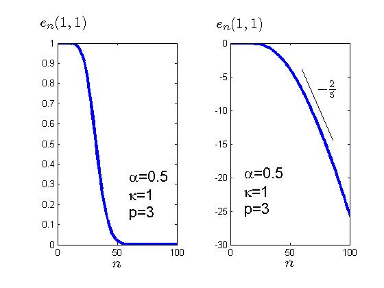
Figure 11: Plot of the relative error $e_{n}(1,1)$ against the number of terms $n$, for $p=3$. Left: Linear-Linear, Right: Linear-Natural Log (y-axis is scaled as $e^{m}$, where $m\in\{-30,-25,\dots,0\}$). A line of slope $-2/5$ is shown for comparison.

These results show that the VIM solutions for this problem convergence rapidly, and actually improves as $n$ increases.

7 Fractional versus Conventional Solutions

In this section, we compare the solutions of the fractional differential Eq. (28) with the corresponding conventional differential equation.

Conventional version of Eq. (28) can be obtained by taking $\alpha=0$, see [41], that is,

$$\frac{\partial{c(x,t)}}{\partial{t}}=\kappa\left[\frac{\partial^{2}c(x,t)}{\partial x^{2}}+\frac{\partial}{\partial x}\left\{xc(x,t)\right\}\right],\quad x>0,t>0.$$ (52)

The solution of Eq. (52) with initial condition $c(x,0)=x$ is

$$c(x,t)=xe^{2\kappa t},$$ (53)

and the general solution for $\alpha>0$ is given by, Section 5.4,

$$c(x,t)=xE_{1-\alpha}[2\kappa t^{1-\alpha}].$$ (54)

Figure 13 shows the plots of the solution (54) for different values of $\alpha$, that also includes the case $\alpha=0$ at $x=1$, for $0<t<1$ and $\kappa=0.4$.

Thus, the relative magnitude of the solutions compared to the conventional case can be estimated from,

$${c^{\alpha}(x,t)\over c^{0}(x,t)}\approx{E_{1-\alpha}[2\kappa t^{1-\alpha}]\over e^{2\kappa t}}.$$ (55)

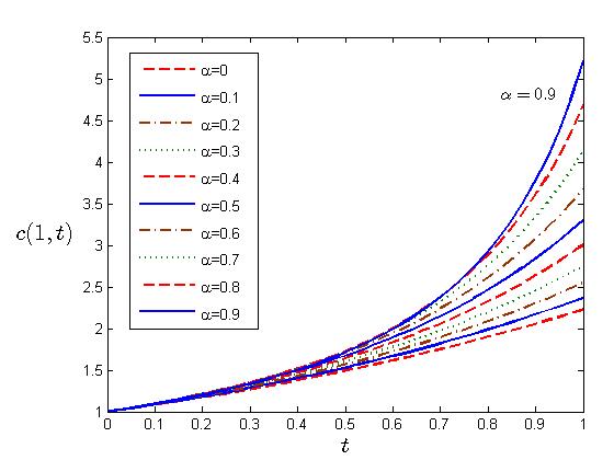
Figure 12: Plot of the solution $c(x,t)$, Eq. (54), when $x=1$, $0<t<1$ and $\kappa=0.4$.

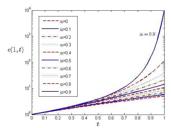
Figure 13: Plot of the solution $c(x,t)$, Eq. (58), when $x=1$, $0<t<1$ and $\kappa=0.4$.

Asymptotic behavior of the above expression can be analyzed through the long time behavior of Mittag-Leffler function. By using Theorem 1.3 of [27], we can write

$${c^{\alpha}(x,t)\over c^{0}(x,t)}\approx\exp\{((2\kappa)^{1/(1-\alpha)}-2\kappa)t\}.$$ (56)

The long time behavior depends on the value of $\kappa$. If $\kappa<1/2$ then ${c^{\alpha}/c^{0}}\to 0$; if $\kappa=1/2$ then ${c^{\alpha}/c^{0}}\to constant$ and the fractional solution scales with the conventional solution; if $\kappa>1/2$ then ${c^{\alpha}/c^{0}}\to\infty$.

The solution of Eq. (52) with initial condition $c(x,0)=x^{2}$ is

$$c(x,t)=x^{2}e^{3\kappa t}+e^{3\kappa t}-e^{\kappa t},$$ (57)

where as, the fractional solution, Example 2 in Section 5.4, is

$$c(x,t)=x^{2}E_{1-\alpha}[3\kappa t^{1-\alpha}]+E_{1-\alpha}[3\kappa t^{1-\alpha}]-E_{1-\alpha}[\kappa t^{1-\alpha}].$$ (58)

Figure 13 shows the plots of the solution (58) for different values of $\alpha$, that also includes the case $\alpha=0$ which corresponds to the classical case, at $x=1$, for $0<t<1$ and $\kappa=0.4$.

The relative magnitude of the solutions compared to the conventional case can be estimated from,

$${c^{\alpha}(x,t)\over c^{0}(x,t)}\approx{x^{2}E_{1-\alpha}[3\kappa t^{1-\alpha}]+E_{1-\alpha}[3\kappa t^{1-\alpha}]-E_{1-\alpha}[\kappa t^{1-\alpha}]\over x^{2}e^{3\kappa t}+e^{3\kappa t}-e^{\kappa t}}.$$ (59)

To leading order, Eq. (59) is,

$${c^{\alpha}(x,t)\over c^{0}(x,t)}\approx{E_{1-\alpha}[3\kappa t^{1-\alpha}]\over e^{3\kappa t}}.$$ (60)

and is easily shown that for general $p>1$, i.e. for initial conditions $c(x,0)=x^{p}$, the corresponding relative magnitude is given by,

$${c^{\alpha}(x,t)\over c^{0}(x,t)}\approx{E_{1-\alpha}[(p+1)\kappa t^{1-\alpha}]\over e^{(p+1)\kappa t}};$$ (61)

and the large time behaviour is,

$${c^{\alpha}(x,t)\over c^{0}(x,t)}\to\exp\{(((p+1)\kappa)^{1/(1-\alpha)}-(p+1)\kappa)t\}\ \ \ \ {\rm as}\ t\to\infty$$ (62)

If $\kappa<1/(1+p)$ then ${c^{\alpha}/c^{0}}\to 0$; if $\kappa=1/(1+p)$ then ${c^{\alpha}/c^{0}}\to constant$ and the fractional solution scales with the conventional solution; if $\kappa>1/(1+p)$ then ${c^{\alpha}/c^{0}}\to\infty$.

8 Conclusion

Some complex physical phenomenon such as crowded systems, and transport through porous media are not fully understood at the present time, and in order to shed new light into such phenomena a new modeling strategy has emerged in recent years which involves casting the system of interest in terms of fractional calculus.

In this study the Hilfer fractional advection-diffusion equation of order $0<\alpha<1$ and type $0\leq\beta\leq 1$,

$$\frac{\partial{c(x,t)}}{\partial{t}}=\kappa\ _{0}\mathcal{D}_{t}^{\alpha,\beta}\left[\frac{\partial^{2}c(x,t)}{\partial x^{2}}-\frac{\partial}{\partial x}\left\{u(x)c(x,t)\right\}\right],\quad x>0,t>0,$$

with advection term $u(x)=-x$, and power law initial conditions of the type $c(x,t=0)=x^{p}$ for $p>0$, was investigated numerically using the Variational Iteration Method (VIM) method, with a view of comparing its solution to the conventional non-fractional advection-diffusion system, and also to analyze the system numerically in order to investigate the efficiency of solving such systems numerically.

For this class of initial conditions $c(x,t=0)=x^{p}$ for $p>0$, the above problem yields the same solutions as Caputo and Riemann-Liouville advection-diffusion equations. However, we remark that this would be different in case if there is a source term in the problem or if the velocity also involves time variable.

Power series solutions were obtained, Eq. (42). These yield closed form solutions for specific $p>0$ in terms of the Mittag-Leffler functions, although it becomes increasingly difficult to actually calculate it for $p>2$. Nevertheless, the leading order term can readily be obtained even for $p>2$, which allows us to investigate the asymptotic behavior of the solutions and to carry out some numerical analysis of the method used. The power series is (absolutely) convergent (for all $x$, and all $t$, and for $p\geq 0$).

The behavior of the solution was examined by comparing the value of the solution at a fixed point, namely $|c(1,1)|$. Asymptotically, the relative magnitude of the solutions is, $|{c^{\alpha}(x,t)\over c^{0}(x,t)}|\approx{E_{1-\alpha}({(p+1)\kappa t})\over e^{(p+1)\kappa t}}$ which shows that the fractional solution increases approximately exponential faster than the conventional solution, as seen in Figs. 13 and 13.

For fixed $p$, the increase in $|c(1,1)|$, when $\alpha\in(0,0.7)$ and $\kappa<\frac{1}{p+1}$, is small; but when $\alpha>0.7$ and $\kappa\geq\frac{1}{p+1}$, $|c(1,1)|$ increases very rapidly. For fixed $\alpha$ and $\kappa$, the solution increases polynomially with $x$ and exponentially with $t$.

For the long time behaviour, as $t\to\infty$, we find that for all $x$ and for all $0<\alpha<1$, if $\kappa<1/(1+p)$ then ${c^{\alpha}/c^{0}}\to 0$; and if $\kappa=1/(1+p)$ then ${c^{\alpha}/c^{0}}\to constant$ and the fractional solution scales with the conventional solution; and if $\kappa>1/(1+p)$ then ${c^{\alpha}/c^{0}}\to\infty$.

Variational iteration method (VIM) has proved to be an efficient method for obtaining the series solution of the Hilfer fractional advection-diffusion equation with the given power law initial data. Truncation errors $\epsilon(n)$, arising when using the partial sum as approximate solutions, decay exponentially fast with the number of terms $n$ used, and then rate of convergence is independent of $p$ for the cases considered, $\epsilon(n)\sim\exp(-2/5)$, for $p=1,2,3$.

The number of terms $n$ required for a given level of accuracy for $\alpha<0.7$ are relatively insensitive to both the $\alpha$ and to the accuracy level required; but for $\alpha>0.7$ the number of terms increases rapidly with $\alpha$ and with the accuracy level required. This threshold $\alpha\approx 0.7$ is consistent with the analysis of the solutions $|c(1,1)|$ above.

Although these are early days in the development of fractional calculus and numerical solutions to fractional equations that describe physical systems, it is clear that numerical methods like VIM will be important tools in extracting solutions of such fractional PDE’s in the future.

Future work will address the case when we have non-zero initial conditions which should yield different solutions for each $\beta$.

Appendix A

In a single-phase single-component system, let us denote the concentration of the scalar by $c(x,t)$ at the position $x$ and at the time instant $t$. First, if $u(x,t)$ is the velocity field in which the scalar is transported, then the advection equation (without reaction or diffusion) is [1],

$$\frac{\partial{c(x,t)}}{\partial{t}}+\frac{\partial}{\partial x}\left\{u(x,t)c(x,t)\right\}=0.$$ (63)

Second, if the concentration $c(x,t)$ is transported by diffusion and these changes are caused by gradients in $c(x,t)$ and the fluxes across the boundaries of the region, then the diffusion equation (without advection or reaction) is [1],

$$\frac{\partial c}{\partial{t}}=-\frac{\partial}{\partial x}\left(J_{c}\right),$$ (64)

where $J_{c}=-d(x,t)\frac{\partial c}{\partial{x}}$ is the flux of $c$ at the point $(x,t)$, and $d(x,t)$ is the coefficient of diffusivity. This form in which the flux $J_{c}$ is proportional to the scalar gradient is called Fickian diffusion.

Finally, there may be local changes in $c(x,t)$ due to sources, sinks, and chemical reactions, which is described by an additional source (reaction) term $f(x,t,c(x,t))$. The reaction equation (without advection or diffusion) is [1],

$$\frac{\partial{c(x,t)}}{\partial{t}}=f(x,t,c(x,t)).$$ (65)

The general advection-diffusion-reaction equation is obtained by combining the above three effects and the overall change in the concentration $c(x,t)$ is described by the following equation [1]

$$\frac{\partial{c(x,t)}}{\partial{t}}+\frac{\partial}{\partial x}\left(u(x,t)c(x,t)\right)=-\frac{\partial}{\partial x}\left(J_{c}\right)+f(x,t,c(x,t)).$$ (66)

Applications of such equations arise in many fields, such as, atmospheric chemistry, [3], air pollution models, [4], climatology, [5], modeling of fluid flow in homogeneous media, [6], catalysis, [7], combustion, [8].

In a similar way nonlinear advection-diffusion-reaction equations are obtained by using nonlinear conservation laws, see [9], [10] and [11] . The nonlinear advection-diffusion-reaction equation has the form

$$\frac{\partial{c(x,t)}}{\partial{t}}+\frac{\partial}{\partial x}P\left(u(x,t)c(x,t)\right)=-\frac{\partial}{\partial x}\left(J_{c}\right)+f(x,t,c(x,t)).$$ (67)

where $P\left(u(x,t)c(x,t)\right)$ represents the non-linear convective flux.

Appendix B

Laplace transform of fractional derivatives

$$\mathcal{L}[_{0}^{*}D_{t}^{\alpha}f(t);s]: =s^{\alpha}\widetilde{f}(s)-s^{\alpha-1}f(0^{+}),\quad 0<\alpha\leq 1,$$ (68)

where

$$f(0^{+}): =\lim_{t\rightarrow 0^{+}}f(t).$$

$$\mathcal{L}[_{0}D_{t}^{\alpha}f(t);s]: =s^{\alpha}\widetilde{f}(s)-\left({}_{0}I_{t}^{1-\alpha}f\right)(0^{+}),\quad 0<\alpha\leq 1,$$ (69)

where

$$\left({}_{0}I_{t}^{1-\alpha}f\right)(0^{+}): =\lim_{t\rightarrow 0^{+}}\left({}_{0}I_{t}^{1-\alpha}f\right)(t)$$

$$\mathcal{L}\left[D_{t}^{\alpha,\beta}f(t);s\right]: =s^{\alpha}\widetilde{f}(s)-s^{\beta(1-\alpha)}\left[{}_{0}I^{(1-\beta)(1-\alpha)}f(0^{+})\right],\quad 0<\alpha<1,$$ (70)

where

$$\left({}_{0}I_{t}^{(1-\beta)(1-\alpha)}f\right)(0^{+}): =\lim_{t\rightarrow 0^{+}}\left({}_{0}I_{t}^{(1-\beta)(1-\alpha)}f\right)(t)$$

Note: One can see that the differences in these Laplace transforms are in the initial data $f(0^{+})$, $\left({}_{0}I_{t}^{1-\alpha}f\right)(0^{+})$, and $\left({}_{0}I_{t}^{(1-\beta)(1-\alpha)}f\right)(0^{+})$.

Lemma 8.1.

[43] Assume that $f(t)$ is continuous on $[0,T]$, for some $T>0$, then

$$\lim_{t\rightarrow 0^{+}}\left({}_{0}I_{t}^{\alpha}f\right)(t)=0,$$

for $\alpha>0$.

References

- [1] W. Hundsdorfer, J.Verwer; Numerical solution of time-dependent advection-diffusion-reaction equations, Springer-Verlag, Berlin, Heidelberg, 2003.
- [2] R.B. Bird, W.E. Stewart, E.N. Lightfoot; Transport phenomena, John Wiley and Sons, Inc., New York, 2002.
- [3] T.E. Graedel, P.J. Crutzen; Atmosphere, climate and change, Henry Holt and Company, 1997.
- [4] B. Sportisse; Air Pollution Modelling and Simulation, Springer-Verlag, Berlin, Heidelberg, 2002.
- [5] T. Stocker; Introduction to Climate Modelling, Springer, new York, 2011.
- [6] K. Aziz, A. Settari; Petroleum reservoir simulation, Applied Science Publishers Ltd., London, 1979.
- [7] E. Cumberbatch, A. Fitt; Mathematical Modeling: Case Studies from Industries, Cambridge University Press, UK, 2001.
- [8] I. Glassman, R.A. Yetter; Combustion, Academic Press, London, San Diego, Burlington, 2008.
- [9] A. Kurganov, E. Tadmor; New high-resolution central schemes for nonlinear conservation laws and convection-diffusion equations, J. Comp. Physics, 160 (2000), 241-282.
- [10] A. Bressan, M. Lewicka, G. Chen, D. Wang; Nonlinear conservation laws and applications, Springer Science, New York, 2011.
- [11] R.J. LeVeque; Nonlinear conservation laws and finite volume methods for astrophysical fluid flow, Computational methods for astrophysical fluid flows, Springer-Verlag, Berlin, Heidelberg, 1998.
- [12] M. Khebchareon, S. Saenton; Finite Element Solution for 1-D Groundwater Flow, Advection-Dispersion and Interphase Mass Transfer : I. Model Development, Thai J. Math., 3 (2005), 223-240.
- [13] G.I. Marchuk; Mathematical Models in Environmental Problems, North-Holland, Elsevier Science Publisher, 1986.
- [14] J.R. Holton, G.J. Hakim; An introduction to dynamic meteorology, Academic Press, USA, 2013.
- [15] E. S. Oran, J. P. Boris; Numerical Simulation of Reactive Flow, Second edition, Cambridge University Press, UK, 2001.
- [16] R. Glowinski, J. Xu; Numerical Methods for Non-Newtonian Fluids, Handbook of Numerical Analysis, Volume 16 (2011), 1-801.
- [17] F.V. Shuhaev, L.S. Shtemenko; Propagation and reflection of shock waves, World Scientific Publishing, Singapore, 1998.
- [18] M. Treiber, A. Kesting; Traffic flow dynamics: Data, Models and Simulation, Springer-Verlag, Berlin, Heidelberg, 2013.
- [19] O. Pironneau, Y. Achdou; Partial differential equations for option pricing, Math. Model. and Num. Methods in Finance, Special Volume, Handbook of Numerical Analysis, 2008.
- [20] J.H. Jeon, V. Tejedor, S. Burov, E. Barkai, C. Selhuber-Unkel, K. Berg-Sørensen, L. Oddershede, and R. Metzler; In vivo anomalous diffusion and weak ergodicity breaking of lipid granules, Physical review letters 106, no. 4 (2011) 048103.
- [21] J. Sabatier, O. P. Agrawal, and J. A. T. Machado, Advances in fractional calculus, Dordrecht: Springer, 2007.
- [22] S.M.A. Tabei, S. Burov, H. Y. Kim, A. Kuznetsov, T. Huynh, J. Jureller, L. H. Philipson, A. R. Dinner, and N. F. Scherer; Intracellular transport of insulin granules is a subordinated random walk, Proceedings of the National Academy of Sciences 110, no. 13 (2013) 4911-4916.
- [23] M. Weiss, M. Elsner, F. Kartberg, T. Nilsson; Anomalous Subdiffusion Is a Measure for Cytoplasmic Crowding in Living Cells, Biophysical J., 87 (2004), 3518-3524.
- [24] W. Chen, H. Sun, X. Zhang, D. Korosak ; Anomalous diffusion modeling by fractal and fractional derivatives, Comp. Math. Appl. 59(5), (2010), 1754-1758.
- [25] K.B. Oldham, J. Spanier; The fractional calulus, Academic Press, New York and london, 1974.
- [26] K.S. Miller, B. Ross; An Introduction to the fractional calculus and fractional differential equations, John Wiley and Sons, Inc., New York, 2003.
- [27] I. Podlubny; Fractional differential equations, Academic Press, San Diego, Calfornia, USA, 1999.
- [28] K. Diethelm, N.J. Ford; Analysis of fractional differential equations, J. Math. Anal. Appl. 265 (2002) 229-248.
- [29] M. Caputo; Diffusion of fluids in porous media with memory, Geothermics, 28 (1999) 113-130.
- [30] S. Havlin, D. Ben-Avraham; Diffusion in disordered media, Advances in Physics, 51(2002), 187-292.
- [31] R. Metzler, J. Klafter; The random walk’s guide to anomalous diffusion: a fractional dynamics approach, Physics Reports, 339 (2000) 1-77.
- [32] S. Das; Analytical solution of a fractional diffusion equation by variational iteration method, Comp. Math. Appl. 57 (2009), 483-487.
- [33] S. Saha Ray, R.K. Bera; Analytical solution of a fractional diffusion equation by Adomian decomposition method, Appl. Math. Comput. 174 (2006), 329-336.
- [34] R. Hilfer; Applications of fractional calculus in physics, World Scientific Publishing Company, Singapore, 2000.
- [35] R. Hilfer; Experimental evidence for fractional time evolution in glass forming materials, Chemical Physics, 284 (2002) 399-408.
- [36] R. Hilfer; On fractional relaxation, Fractals 11 (2003) 251-257.
- [37] R. Hilfer, Foundations of fractional dynamics: a short account, Fractional dynamics: recent advances. World Scientific, Singapore 207 (2011).
- [38] T. Sandev, R. Metzler, Z. Tomovski; Fractional diffusion equation with a generalized Riemann-Liouville time fractional derivative, J. Phys. A: Math. Theor. 44 (255203) (21pp), (2011).
- [39] R. Metzler, and J. Klafter, The restaurant at the end of the random walk: recent developments in the description of anomalous transport by fractional dynamics, Journal of Physics A: Mathematical and General 37, no. 31 (2004): R161.
- [40] Ž. Tomovski, T. Sandev, R. Metzler, and J. Dubbeldam, Generalized space–time fractional diffusion equation with composite fractional time derivative, Physica A: Statistical Mechanics and its Applications 391, no. 8 (2012): 2527-2542.
- [41] A.A. Kilbas, H.M. Srivastava, J.J. Trujillo; Theory and Applications of Fractional differential equations, North-Holland, Elsevier Science Publisher, 2006.
- [42] H. M. Srivastava, Ž. Tomovski; Fractional calculus with an integral operator containing a generalized Mittag–Leffler function in the kernel’ Applied Mathematics and Computation 211.1 (2009): 198-210.
- [43] K. M. Furati, M. D. Kassim, N. -e. Tatar; Non-existence of global solutions for a differential equation involving Hilfer fractional derivative, Electronic Journal of Differential Equations 2013.235 (2013): 1-10.
- [44] A.M. Wazwaz; Partial differential equations and solitary waves theory, Springer, New York, 2009.
- [45] Y. Liu, X. Zhao; He’s Variational Iteration Method for Solving Convection Diffusion Equations, Advanced Intelligent Computing Theories and Applications, Lecture Notes in Computer Science, Springer, New York, 6215 (2010) 246-251.
- [46] Y. Molliq R., M.S.M. Noorani, I. Hashim; Variational iteration method for fractional heat- and wave-like equations, Nonlinear Analysis: Real World Apllications, 10(2009) 1854-1869.
- [47] S. Momani, Z. Odibat; Comparison between the homotopy perturbation method and the variational iteration method for linear fractional partial differential equations, Comp. Math. App., 54(2007) 910-919.
- [48] J.H. He; Approximate analytical solution for seepage flow with fractional derivatives in porous media, Comput. Methods Appl. Mech. Engrg. 167 (1998) 57-68.
- [49] J.H. He; Variational iteration method: a kind of non-linear analytical technique: some examples, Int. J. Non-Linear Mech., 34 (1999) 699-708.
- [50] F. Qi; Bounds for the ratio of two Gamma functions, J. Ineq. App., Volume 2010, Article ID 493058, 84 pages.
- [51] H. Alzer; Sharp upper and lower bounds for the gamma function, Proceedings of the Royal Society of Edinburgh: Section A Mathematics, Appl. Numer. Math. 139 (2009), 709-718.