School of Mathematics and Statistics, University of Sydney
Stochastic Analysis Seminar on Filtering Theory
Author:
Andrew Papanicolaou
alpapani@maths.usyd.edu.au
These notes were originally written for the Stochastic Analysis Seminar in the Department of Operations Research and Financial Engineering at Princeton University, in February of 2011. The seminar was attended and supported by members of the Research Training Group, with the author being partially supported by NSF grant DMS-0739195.
Chapter 1 Hidden Markov Models
We begin by introducing the concept of a Hidden Markov Model (HMM). Let denote time, and consider a Markov process which takes value in the state-space . We assume that the distribution function of has either a mass or a density, and we denote mass/density with such that
for any and . The generator of is the operator with domain , such that for any bounded function we have a backward equation,
for any . Provided that regularity conditions are met, the adjoint leads to the forward equation,
Example 1.0.1.
If (a finite space) and the operator is a jump-intensity matrix such that for all and for all . The forward equation is then
Example 1.0.2.
If and is an Itô process such as
then is the generator. The backward equation is then
for any bounded function . Provided that and the initial distribution satisfy some conditions for regularity, there is also a forward equation given by the adjoint
for any .
In addition to , there is another process that is a noisy function of . The process can given by the SDE
where is an independent Wiener process, or can be given discretely,
where is a set of discrete times at which data is collected.
As a pair, are a Markov chain. The process is of primary interest to us and is referred to as the ‘signal’ process, however it is not observable. Instead, the process is in some way observable and so we call it the ‘measurement.’ Hence, is an HMM and the goal is to calculate estimates of that are optimal in a posterior sense given observations on .
1.1 Basic Nonlinear Filtering
Let denote the filtration generated by the observations on up to time . The optimal posterior estimate of in terms of mean-square error (MSE) is
Proposition 1.1.1.
is the unique -measurable minimizer of MSE.
Proof.
Let be another -measurable estimate of . Then
with equality holding iff almost everywhere.
∎
The filtering measure is defined as
for any Borel set , and for any measurable function
Remark 1.
There are also smoothing and prediction distributions. When posteriors have density, we write
We say that is the smoothing density if and the prediction density if . Smoothing requires significantly more calculation to compute, but the prediction simply requires us to solve the forward equation for in the interval with initial condition .
Example 1.1.1.
Filtering With Discrete Observations; The Bayesian Case. Let be a countable state-space, let be a known nonlinear function, let , and for let there be specific times at which observations are collected on . At each time , let and denote the history of measurements up to time as . Denote .
Consider the following discrete differential:
where and .
Using Bayes rule, we find the the filtering distribution has a mass function
for any . It can be written recursively as follows,
| (1.1) |
where is the kernel of ’s forward transition probabilities, is the likelihood ratio of given ,
and is a normalizing constant. Equation (1.1) can be shown to hold true through a use of Bayes formula and by the independence properties of the HMM.
Proof.
(of equation (1.1)) Regarding the likelihood function of given , it is
and since we are only interested in how this likelihood varies with , we can remove the terms that do not have in them,
and so it is in fact the likelihood-ratio of .
Now, by Bayes formula we have,
and clearly, is the integral of numerator of the last line over . ∎
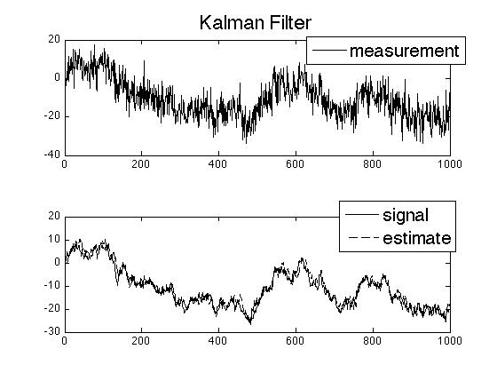
The Bayesian filter is an essential tool for numerical computations of nonlinear filtering. The Kalman filter (see Jazwinski [28]) is also an important tool, but it only applies to linear Gaussian models or models that are well-approximated as such. The contemporary way to compute nonlinear filters is via Monte Carlo with a particle filter (which we’ll talk about in a later section). In continuous time, approximating filters based on discretization of the differential have been shown to converge as for a certain class of filtering problems, but we must be able to approximate the law of , and must be bounded (see Kushner [33]).
In summary, an HMM consists of a pair of process where is an unobserved signal which is a Markov process, while is an observable process that depends on through a system of known functions and known parameters. We use filtering to compute the posterior distribution of given .
Chapter 2 Filtering and the VIX
2.1 Stochastic Volatility
Consider an equity model with stochastic volatility,
where is the price of a stock, the function is known and is a hidden Markov process. For instance, the Heston model, where and
where we model the volatility leverage effect by saying that with .
In general, if we observe a continuum of prices, then is measurable with respect to the filtration generated by . Let , and notice that
For a fixed , let be a partition of , then the quadratic variation of is the cumulative variance
where . Clearly, then is -measurable, and if is a continuous process we have
is also -measurable. So at the very least (e.g. for a continuous process) volatility is observable for almost everywhere , and is observable if exists.
Nonetheless, it is still beneficial to have a Markov structure for so that we can price derivatives on . For instance, in the example by Elliot [22], the Black-Scholes price of a European call option in the presence of Markovian volatility, when is
where , and is the market’s pricing measure. Given and the parameters of ’s dynamics under the market measure, we can compute the expected return of the call option either explicitly or through Monte Carlo.
If is not known (i.e. observations are discrete) then we could take a filtering expectation,
but such a price would be significantly biased if the market placed any premium on volatility. This option pricing formula exemplifies the challenge of interpreting the filter in financial math.
2.2 The VIX
Filtering can be used to extract the risk-premium placed on volatility by the market. Let be the S&P500 index. For any time and some time-window , the VIX index is the square root of the market’s prediction of average variance during ,
where is the market’s pricing measure, and is the filtration generated by all the information in the market (i.e. ). The process is the ‘fair’ price of a variance swap whose floating leg is the realized variance,
where is a partition of (i.e. , with going to zero as gets large). For a pre-specified notional amount, the payoff of a variance swap is
2.2.1 The VIX Formula
For diffusion models without jumps, it was shown by Demeterfi et al [19] that a portfolio of out-of-the-money call and put contracts along with a short position in a futures contract replicates the VIX. It was shown by Carr et al [14, 15] that models with jumps can be approximated by the same setup. The following lemma derives the strategy for diffusions:
Lemma 2.2.1.
Let denote the life of the contract, let denote the future price on at time , and let be the rate so that . If is purely a diffusion process (i.e. has no jump terms in its differential), then the market’s expectation of future realized variance is
| (2.1) |
where and denote the price of a put and a call option at time with strike and time to maturity , respectively.
Proof.
Under the market measure, there is a Wiener process such that the returns on the stock satisfy
and the log-price satisfies
Integrating the returns and the log-price separately and then subtracting, we can eliminate all randomness to get the cumulative variance,
which shows us that the realized variance satisfies the following:
Then, through some simple calculus, we see that
Plugging this expression for into we see that the realized variance can be written as the payoffs of several contracts and a continuum of puts and calls that were out-of-the money at time :
Taking expectation of both with respect to the market measure, the noise in vanishes, and since both and , we have
and if we multiply and divide the RHS by we get the result. ∎
Risk Premium
Under the market measure, the expected returns on a variance swap are zero. However, statistically speaking, variance swaps exhibit a slight bias against the holder of the contract. In other words, the person who receives at time will have an average return that is slightly negative. But because of the volatility leverage effect, the variance swap has the potential to provide relief in the form of a positive cash flow when volatility is high and equities are losing. When quoted in the market, the VIX is quoted as the square-root of in percentage points, and is a mean-reverting process that drifts between 15% and 50%. The VIX has the nickname ‘the investor fear gauge’, as it should because it is composed primarily of out-of-the-money options which means that there is an increase in crash-a-phobia whenever the VIX increases.
To get a more precise understanding of investors’ fears, it would be nice to remove any actual increases in volatility and merely examine the bias in the market measure’s prediction of variance. In other-words, we would like to predict variance in the physical measure, and then compare it with the VIX’s prediction to gain a sense of how much of a premium is being placed on risk, or how much fear there is out there.
If we can identify an HMM whose observable component generates , then the market’s price of volatility risk (aka the risk-premium) is
Remark 2.
Carr and Wu [16] point out that if we define the martingale change of measure with the Radon-Nykodym derivative , then
where and , which leads to an expression for the risk-premium, and is -measurable provided that is known.
More on the VIX
Historically, indices like the S&P500 exhibit contrary motion with volatility. In particular, periods of high volatility often coincide with bearish markets. Whaley [46] describes how tradable volatility assets, such as the VIX, provided market makers with new ways to hedge the options they had written. For instance, a market maker who was short a portfolio of options has always been able to go long in some other types of contracts to reduce the portfolio’s Delta to almost zero, meaning that the portfolio would not be hugely affected by small changes in the value of the underlying. When VIX was introduced, it allowed the same market maker the opportunity to also hedge the Vega of his/her short position in options. Prior to volatility hedging instruments, a market maker might be exposed to the rising options prices that occur as volatility increases. However, instruments such VIX futures and calls on VIX futures changed all that, as a short position in options could then have its Vega reduced to almost nothing with the appropriate number of VIX contracts.
Traders use VIX futures and options to hedge in times of uncertain volatility in the SPX or the SPY.111SPX is the S&P500; SPY is the tracking stock for the S&P 500. When volatility traders notice a spread between the VIX and VIX futures, they realize that a correction is probable. Therefore, if VIX is trading higher than the VIX futures price, then buying calls in both SPY and VIX will make money because either a) VIX goes down and the SPY goes up which places the SPY call in-the-money, or b) the VIX stays up and the VIX futures close the gap which places the VIX call in-the-money. A similar strategy with puts on SPY and VIX can be devised when the VIX is significantly lower than the VIX futures price. The rule of thumb is: provided that the spread between VIX and VIX futures is wide enough, the correction in VIX will create enough change in the market that one of these straddles can cover its initial cost and provide some profit to the investor. The operative word in the strategy mentioned in this paragraph is spread, which is precisely what we are looking for as we filter for the risk-premium.
Chapter 3 Stochastic Volatility Filter for Heston Model
With discrete observations, we derive a Bayesian stochastic volatility filter for a Heston model. Let denote the log-price of the equity, and let denote volatility. The dynamics of the processes are,
| (3.1) | |||||
| (3.2) |
and the interpretation of the model parameters is as follows:
| the long-time average of | ||||
| the rate of mean-reversion (on ) | ||||
| volatility of volatility | ||||
| models volatility leverage effect when | ||||
| the mean-rate of returns on the stock |
Certain restrictions on the parameters need to be put in place, such as the Feller condition: to insure the is well-defined (see chapter volatility time scales in [24]). There are times for which the process is actually observed, and if our model is correct111‘correct’ not only means that the processes follow these parametric SDEs, but it also means that and are idiosyncratic noises that are endemic to this system and not correlated with other data in the market. then .
3.1 The Filter
We showed in previous lectures that is measurable when is observed continuously. It is also straight forward to show that as the partition of shrinks to zero.
Lemma 3.1.1.
Proof.
Let . We assume that the filtrations are increasing with , and they are certainly bounded by ,
Therefore there exists such that . Now because the path of is continuous on all sets of non-zero probability, the information contained in is enough to measure the event for any even if is not a partition point for any finite . Therefore, a.s., and by the Lévy 0-1 law we have
which proves the lemma.
∎
From lemma 3.1.1 we know that our posterior estimates are consistent as we refine the partition. Now we need to determine the filter for a specific partition. From here forward consider a specific finite partition of the time domain, and we only consider the filter at times when data has arrived. For ease in notation we let , and .
Proposition 3.1.1.
Let be the price and volatility processes in the Heston model from (3.1) and (3.2), and assume the Feller condition . Then there is a kernel that gives ’s transition density, for any , and the filtering distribution for at observation time has a density. This density is given recursively as
| (3.3) |
for almost-everywhere , where is a normalizing constant, and is the likelihood of the any path given observations and , and is given by
with
Proof.
Given the Feller condition, the CIR process is well-known to have a transition density that can be written in terms of a modified Bessel function (see [1]), and so is a smooth density function for all . Furthermore, it was shown in [20] that has a smooth transition density function, that is,
is smooth for , , and , and does not collect mass at or . Hence, the filter has a density that can be written using Bayes rule:
where we don’t need to assume smoothness of because it is smoothed by its convolution with in the -integral.
Now, from equation (3.2) we notice the following:
where “” signifies equivalence in distribution, and is another independent standard normal random variable. This means that conditional on the path and ,
Then noticing evaluated at is the the same as , it follows that
This shows the likelihood of the path given and is in fact the function .
Finally, given Bayes rule for the density , the expression in equation (3.3) displays the filter using a probabilistic representation of the transition density:
Lastly, when computing the likelihood based on the time- observation, the last line is evaluated at . This completes the proof of the proposition.
∎
At this point it seems that the filter is rather complicated, and would be difficult to implement in real-time. Often times, what one might do is consider a discrete scheme that approximates the SDEs:
| (3.4) | |||||
| (3.5) |
where and . Using (3.4) and (3.5), we can impute an approximate filtering density to the density given in Proposition 3.1.1:
| (3.6) |
where is the likelihood of given ,
If the model simplification given by (3.4) and (3.5) can be considered ‘correct’, then there is no need to dispute the validity of the filter given by (3.6). But in general, if one knows apriori that the continuous-time SDEs are the correct model, then there needs to be some analysis to verify that the approximate filter (such as that in(3.6)) converges as , that is
in a strong sense as . As was mentioned earlier, it is well-known (see Kushner [33]) that approximate filters that are sometimes consistent, but the results in [33] do not apply to the Heston model.
3.2 Extracting the Risk-Premium
Under the physical measure, we have,
and so the expected value of realized variance () is
where we have (without loss of generality) considered the case at time 0, and we have denoted the posterior expectation as and . Therefore, there is the following close-formula for the risk-premium
This expression for the risk-premium holds whenever volatility-squared is modeled with a mean-reverting SDE with drift term , not just the Heston model.
Under the risk-neutral measure, the market adds a risk-premium term to :
where Brownian motion under the market measure, and is the market price of volatility risk. We leave the modeling of open here because we will not delve deeply into its correlation structure. However, is most likely thought of as a mean-reverting process and could be modeled as such. Under the market’s measure there is the following expectation of variance
From this, we see that can be written as follows,
In , notice that if and are independent, then for the risk-premium simplifies to
3.3 Filtering Average Volatility in Fast Time-Scales
The purpose of fast time-scales in volatility modeling is to capture mean reverting effects that occur on the order of 2 to 3 days. In the Heston model, suppose we are in a fast time-scale where for large. Then, it can be shown that the distribution of settles into a distribution almost instantaneously,
for all . Therefore, there is a fast-averaging of the realized variance,
and so the expected payoff of any contract that is a function of realized variance will be deterministic unless is random and/or unknown. Thus, building a risk-premium into the dynamics of in the manner that we did in the previous section will not be meaningful in fast time-scales. An alternative idea would be to take as a hidden regime-process that is governed by another Markov chain, and thus adds another dimension to the HMM. Then, we can take realized variance as our observations and write a filter to estimate the regime . We do this as follows:
Take to be a Markov chain with generator , for which we assume the standard structure for changes; changes in are governed by a Poisson jump process so that over a time interval of length , the probability of changing states more than once is . The new dynamics of are then
and for such a model the realized variance is a random variable in fast time-scales,
Let be a partition of some finite time interval, say years, where denotes the week, and denotes the trade. Then
We have observations on at each (i.e. is the observations on the week). For any and let , and for simplicity let . We then have the following model for weekly observations on realized variance,
where is a noise process with if . Clearly, is observable and is a Markov process. From here the goal is to estimate the the state-space and transition rates of , and then apply the nonlinear filtering results in estimating the variance risk-premium. Letting , we have an estimate of the physical measure’s expectation of realized variance:
for .
Chapter 4 The Zakai Equation
Let be a Markov process with generator . Let the domain of be denoted by , and let denote the subset of bounded functions in . For any function we have the following limit:
as , for any . If is densely-defined and its resolvent set includes all positive real numbers, then the Hille-Yosida theorem applies, allowing us to write the the distribution of with a contraction semi-group. In these notes we assume that such conditions hold and that the transition density/mass is generated by an operator semigroup denoted by .
A standard nonlinear filtering problem in SDE theory assumes that is unobserved and that a process is given by an SDE
| (4.1) |
where is an independent Wiener process, and we assume that is bounded for all .
The pair is an HMM for which filtering can be used to find the posterior distribution. Let , and for any measurable function let
The posterior expectation of is ultimately what is desired from filtering, but the methods for obtaining the posterior distribution are quite involved. The discrete Bayesian tools that we’ve used in earlier lectures cannot be used here because we are in a continuum that does not allow us to break apart the layers of the HMM. Instead, we will exploit well-known ideas from SDE theory to obtain the differentials for the filtering distribution. In particular, we will use the Girsanov theorem to obtain the Zakai equation.
4.1 Discrete Motivation from Bayesian Perspective
In their book, Karatzas and Shreve [30] give a discrete motivation for how the Girsanov theorem works. In a similar fashion, we consider a discrete problem and then construct a change of measure from the ratio of the appropriate densities. We then show how it is analogous to its continuous-time counterpart, and leads to a discrete approximation of the Zakai equation.
To do so, we start by considering a discrete-time analogue of (6.1),
and assume that the unconditional distribution of is a density for all (the same idea will be applicable when ’s distribution has a mass function). We can easily apply Bayes theorem to obtain the filtering distribution on a Borel set :
where represents kernel of ’s transition densities, the likelihood function is
and is a normalizing constant. The Lebesgue differentiation theorem can be applied to obtain the density of the posterior,
when shrinks nicely to .
Keeping this discrete model and filter in mind, let’s shift our attention to a joint density function of all observations and a possible path taken by ,
where can be obtained using the exponential of .
Next, consider an equivalent measure in where is Brownian motion independent of , and the law of remains the same. Under this new measure the joint density function is
The ratio of these densities is written follows:
which is the likelihood ratio of any path for the discrete observation model. It is also the discrete analog of the exponential martingale that we use in the Girsanov theorem. Furthermore, we can use to rewrite the filtering expectation in terms of the alternative measure,
and if we define we can write the filtering expectation as
for any function .
It turns out to be advantageous to analyze under -measure because the dynamics are linear when we move to a continuum of observations. To get a sense of the linearity, consider the following discrete expansion for small ,
because by a discrete interpretation of Itô’s lemma, and is -measurable. Now, because is independent of under , the conditioning up to time is superfluous and we can reduce it down to time ,
Then we can again exploit the independence of from under and use an approximation of ’s backwards operator.
and then using the fact that , we have
which foreshadows the Zakai equation in a discrete setting,
4.2 Derivation of the Zakai Equation
In this section we use the Girsanov theorem as the main tool in a formal derivation of the nonlinear filtering equations in continuous time. For ease in notation we let , but this does change the results because the would merely need to be rewritten to include the time dependence in .
We start by considering the finite interval and defining the following exponential,
for all . Since it was initially assumed that was independent, we can define an equivalent measure by
By the Girsanov theorem we know that
-
1.
is a probability measure, and
-
2.
is -Brownian motion for , conditioned on .
It is easy to show with moment generating functions that . We can also easily show that is a true -martingale,
Lastly, a simple lemma shows that and are path-wise independent under :
Lemma 4.2.1.
and are path-wise independent under .
Proof.
For an arbitrary path-wise function we have
showing that is -Brownian motion unconditional on . Then for another arbitrary path-wise function we have
and so and are -independent. ∎
From here forward, define the measure on as
With this new measure we can express another important result regarding the Girsanov change of measure, namely the Kallianpur-Streibel formula:
Lemma 4.2.2.
Kallianpur-Streibel Formula:
for any .
Proof.
For any we have
and since was an arbitrary set, this shows that the result holds wp1. ∎
Now, for any , we use Fubini’s theorem to bring the differential inside the expectation, and from there we apply Itô’s lemma, which gives us the following differential,
for any . From this we can construct the integrated form of the differential,
and since is independent of under the -measure, we can reduce the filtrations from to for all , giving us,
| (4.2) |
for all . Inserting in (4.2) wherever possible and then taking the differential with respect to , we have the Zakai equation:
| (4.3) |
for all . The Zakai equation can also be considered for general unbounded functions , but we have restricted ourselves to the bounded case in order to insure that is finite almost surely. Existence of solutions to (4.3) is straight-forward because we have derived it by differentiating . Uniqueness of measure-valued solutions to (4.3) has been shown by Kurtz and Ocone [32] using a filtered martingale problem, and by Rozovsky [42] using a Radon measure representation of .
4.2.1 The Adjoint Zakai Equation
Depending on the nature of the filtering problem, the unnormalized probability measure may have a density/mass function. For example, suppose that is a diffusion process satisfying the SDE
where . Then the generator is and the Zakai equation is
for any bounded function with a 2nd derivative. Depending on and the initial conditions, may be a density so that
and provided that certain regularity conditions are met, the adjoint of the Zakai equation gives us an SPDE for ,
| (4.4) |
with the initial condition , and with the adjoint operator given by . Existence and uniqueness of such densities is beyond the scope of these notes. Readers who are interested in regularity of solutions should read the book by Pardoux [37].
In the case of filtering distributions that are composed of mass functions, the adjoint equation is similar. For instance, if is a finite-state Markov chain with generator , the adjoint equation holds without any regularity conditions,
General existence and uniqueness for in this discrete case was shown by Rozovsky [41].
4.2.2 Kushner-Stratonovich Equation
Using the Zakai equation of (4.3) and observing that our assumption that is bounded implies for all , we can apply Itô’s lemma to obtain
| (4.5) |
However, it should be mentioned that (4.5) was originally obtain a few years before the Zakai equation using other methods. Under the appropriate regularity conditions, the Kushner-Stratonovich equation is the adjoint (4.5) and is the nonlinear equation for the filtering distribution,
where is either a density or a mass function (depending on the type of problem).
4.2.3 Smoothing
The smoothing filter has been derived in [10], but in the case of regularized processes where the adjoint Zakai equation holds. In this section we derive a similar results but for the general case of functions in , and we’ll also derive the backward SPDE for smoothing in the regularized case.
Consider the times and such that . The filtering expectation of is
For fixed and for increasing, the Zakai equation is
This equation can be solved to obtain the smoothing distribution, but lacks a differential formula for changes in . However, in the regular case there is a backward SPDE that will provide a differential for changes in . This backward SDE will provide improved efficiency for coding and analysis.
Suppose there is sufficient regularity so that satisfies the adjoint Zakai equation (see equation (4.4)). Given , the smoothing filter for any time is
where is define as
The function is the smoothing component and satisfies the following backward SPDE
or in integrated form
Chapter 5 The Innovations Approach
Let be a Markov process with generator . Let the domain of be denoted by , and let denote the subset of bounded functions in . For any function we have the following limit:
as , for any . If is densely-defined and its resolvent set includes all positive real numbers, then the Hille-Yosida theorem applies, allowing us to write the the distribution of with a contraction semi-group. In these notes we assume that such conditions hold and that the transition density/mass is generated by an operator semigroup denoted by .
A standard nonlinear filtering problem in SDE theory assumes that is unobserved and that a process is given by an SDE
| (5.1) |
where is an independent Wiener process, and we assume that the is bounded. Let the filtration so that for an integrable function we have
for all .
5.1 Innovations Brownian Motion
Let denote the innovations process whose differential is given as follows
with , and where .
Proposition 5.1.1.
The process is an Brownian motion.
Proof.
Is is clear that is (i) -measurable, continuous and square integrable on . To show that it is a local martingale, we take expectations for any as follows
Furthermore, the cross-variation of is the same as the cross-variation of , and so by the Lévy characterisation of Brownian motion (see Karatzas and Shreve [30]), is also Brownian motion.
∎
Given that is -Brownian motion, it may seem obvious that any -integrable and measurable random variable has an integrated representation in terms of , but it is not easily seen that . The following proposition provides a proof to verify that it is indeed true.
Proposition 5.1.2.
Every square integrable random variable that is -measurable, has a representation of the form
where is progressively measurable and -adapted and .
Proof.
For all , define . Clearly, is an -martingale, and so we can define an equivalent measure with the following Radon-Nikodym derivative,
As a consequence of the Girsanov theorem, is a -Brownian motion. Then apply the martingale representation theorem,
where is adapted and . From here we can construct a -martingale from ,
and applying Itô’s lemma to we have
Integrating from to , we have
and therefore, setting for all , we have a unique -adapted representation in terms of , and the proposition is proved.
∎
5.2 The Nonlinear Filter
In deriving the nonlinear filter with the innovations Brownian motion, it will be important to use the following martingale for any given :
for all .
Lemma 5.2.1.
is an -adapted martingale.
Proof.
It suffices to show that for any , which we do as follows:
∎
Knowing that is an -martingale, we will apply proposition 5.1.2 as follows
where is an -predicable process for any . From here, the main point in the derivation of the nonlinear filter is in finding the function in terms of quantities that are more readily computable.
Theorem 5.2.1.
The Nonlinear Filter. For any function , the nonlinear filter is given by the following SDE
for all .
Proof.
We can apply proposition 5.1.2 to and we get
thus defining the conditional expectation at time as
From here, to complete the proof only requires us to identify explicitly. For some process , define such that
with . We then apply Itô’s lemma to the following
| (5.2) | |||||
| (5.3) |
If we integrate the integrands in (5.2) and (5.3) from time to time , take expectations, multiply both sides by , and then subtract one from the other, and we are left with
Hence, for almost every , we have
and since belongs to a complete set, must have
which proves the theorem. ∎
Existence of the solutions to the filtering SDE in theorem 5.2.1 is consequence of the fact that is on such solution. The uniqueness of solutions to the filtering SDE can be grouped in with proofs for uniqueness of Zakai equation (see Kurtz and Ocone [32] or Rozovsky [42]) because there is a one-to-one relationship between measure-valued solutions of the two SDEs.
5.2.1 Correlated Noise Filtering
Suppose that and are correlated so that for any function we have
where and the limit is taken as . Then there is an added term in equation (5.3),
and so for almost every we have
and so , and the nonlinear filter is
5.2.2 The Kalman-Bucy Filter
Another big advantage to the innovations approach is in linear filtering. In particular, the case when the filtering problem consists of a system of linear SDEs. In this case, one needs to take some steps to verify that the filtering distribution is normal, but after doing so it is straight-forward to derive equations for the posterior’s first and second moments.
Consider a non-degenerate linear observations model such that and , with being Gaussian distributed, and with state-space generator
for all functions , where and are constant coefficients. The process
is square-integrable and a martingale, and if we extend proposition 5.1.2 for (see proposition 2.31 on page 34 of Bain and Crisan [5]), we can then write using innovations Brownian motion,
where and is -adapted. Now, by simple stochastic calculus we can verify that is given by
where (i.e. the state-space noise is independent of the observation noise). Defining the estimation error as
and applying Itô’s lemma, we have
which has a solution given by the integrating factor,
which is Gaussian distributed and uncorrelated with
for all . Now observe the following:
-
•
are jointly Gaussian for any ,
-
•
is Gaussian and a linear function of ,
-
•
therefore, are jointly Gaussian for any
-
•
in particular are jointly Gaussian and uncorrelated for any .
Therefore, is independent of (for a more detailed discussion see [5, 36]), and so the filter is Gaussian .
If we apply the filter in theorem 5.2.1 with , it yields , and an SDE for the evolution of the first filtering moment
| (5.4) |
We can also apply Itô’s lemma and then take expectations, which will result in a Riccati equation for the evolution of the filter’s covariance,
| (5.5) | |||||
where we have used the fact that , and . Equations (5.4) and (5.5) are the Kalman filter.
Chapter 6 Numerical Methods for Approximating Nonlinear Filters
In practice, the exact filter can only be computed for models that are completely discrete, or for discrete-time linear Gaussian models in which the Kalman filter applies. In the other cases, the consistency of approximating schemes can be relatively trivial, while for others there is a fair amount of analysis required. In this lecture we present the general theory of Kushner [33] regarding the consistency of approximating filters, and also the Markov chain approximation methods of Dupuis and Kushner [21]. But first we present the following simple result regarding filter approximations:
Example 6.0.1.
Let be an unobserved Markov process, and let the observation process be given by an SDE
where is an independent Wiener process, and . For any partition of the interval into -many points, let , and let the filtration generated by the continuum of observations be denoted by . Assuming that
then from the continuity of we know that . Then, by Lévy’s 0-1 law we know that the conditional expectations converge,
for any integrable function . This clearly shows that the filter with discrete observations can be a consistent estimator of the filter with a continuum of observations. However, computing the filter with discrete observations may still require some approximations.
6.1 Approximation Theorem for Nonlinear Filters
In this section we present a proof of a theorem that essentially says: filtering expectations of bounded functions can be approximated by filters derived from models who’s hidden state converges weakly to the true state. The theorem is presented in the context of continuous-time process with a continuum of observations, but can be reapplied in other cases with relatively minor changes.
For some and any , let be an unobserved Markov process with generator with domain , and let denote the subset of bounded functions in . For any function , we have the following limit
as . The observed process is is given by an SDE
| (6.1) |
where is an independent Wiener process, and is a bounded function. For any time , let . From our study of Zakai equation we know that we can write the filtering expectation as
| (6.2) |
where the paths of have the same law as those of but are independent of , and with being the likelihood ratio
The Zakai equation can provide us with an SDE for filtering expectations, but direct numerical quadrature methods to compute the Zakai equation may be difficult to justify.
6.1.1 Weak Convergence
In order to approximate the nonlinear filter, we will look to approximate with a family of process which converge weakly to . Let be a family of measures on a metric space .
Definition 6.1.1.
Weak Convergence. is said to converge weakly to if
for any bounded continuous function . For the induced processes , we denote weak convergence by writing .
Definition 6.1.2.
Tightness. We say that the family of measures is tight if for any there exists a compact set such that
If so we also say that the induced processes are tight.
An important result regarding tightness is Prokhorov’s theorem:
Theorem 6.1.1.
Prokhorov. If is a complete and separable metric space, then the family contained in the space of all probability measure on is relatively compact in the topology of weak convergence iff it is tight.
For the purposes of our study, we will consider processes which are right continuous with left-hand limits (cádlág). Let denote the space of cádlág functions from to , equipped with Skorohod topology. If a family of probability measures is tight, then weak convergence of to the measure on can be shown by verifying that the laws of the induced processes converge to the law of solutions to the associated martingale problem
in probability as for any , and for any . It can be shown that the law of the solution to this martingale problem is unique.
Given a family of measure , an extremely useful tool is the Skorohod Representation Theorem, which says the following:
Theorem 6.1.2.
Skorohod Representation. Let be a family of measures on a complete and separable metric space. If converges weakly to , then there is a probability space with random variables and for which
-
•
for all and any set ,
-
•
for any set ,
-
•
and -a.s. as .
6.1.2 Consistency Theorem
Let be a family of random variables on the same probability space as , which also converge weakly to . Let denote a copy of that is independent of , let the approximated likelihood be denoted by ,
and define the approximated filtering expectation
| (6.3) |
for any function . We then have the following theorem:
Theorem 6.1.3.
Given a family of process taking values in which converge weakly in the Skorohod topology to , the approximated filter in (6.3) will converge uniformly
in probability and in mean as , for any function .
Proof.
(taken from [33]) For the purposes of this proof, we can neglect the terms in and . Let and be bounded processes independent of , and consider the following estimate,
| (6.4) |
We will use the following inequality that holds for real numbers and ,
| (6.5) |
For any real-valued sub-martingale , we have the following inequality (see [30]),
| (6.6) |
Inequality (6.5) and a Schwarz inequality applied to (6.4) yields,
| (6.7) |
By (6.6) the first term in (6.7) is bounded by . To bound the second term we use the fact that
along with (6.6) and the fact that are bounded sub-martingales. Using these facts we can find a constant that depends on , and , such that
| (6.8) |
To prove the theorem is suffices to show that
in probability as . From the boundedness of and , we know that
| (6.9) |
Let be a copy of that is independent of . By the Skorokhod representation theorem we can assume W.L.O.G. that are defined on the same probability space as , that each is independent of , and that a.s. In fact, because we have assume that converges to a continuous function on the Skorohod topology, we know that the convergence is uniform,
as . In particular, a.s.
Taking expectations, we have
Corollary 1.
To generalize theorem 6.1.3 for any such that , we simply need to rework the end of the proof to show that the limit holds pointwise,
in probability and in mean as , almost everywhere , and for any function .
6.2 Markov Chain Approximations
Theorem 6.1.3 applies directly when observations are available as often as needed. In addition, a continuum of observations allows us a certain amount of flexibility in our choice of approximation scheme.
6.2.1 Approximation of Filters for Contiuous-Time Markov Chains
Let be a finite-state Markov chain. Consider a time step . For finite, take and denote the Markov chain with transition probabilities
for any . The Markov chain is discrete but could be extended to by taking , but this is not a continuous-time Markov chain. The non-Markov structure of does not prevent us from applying theorem 6.1.3, but showing tightness and convergence of the martingale problem will be easier if we can find a Markovian approximation.
Let , take , and set with . Now let be the discrete Markov chain that we have already defined, but now consider all up until . A continuous-time approximation of is then
To show that is compact in we proceed as follows:
Take any and for any let denote the time of the jump,
with . For general these ’s may by infinitesimally small, but they will be informative for processes which approximated continuous-time Markov chains.
Next, for any define the set
We can easily check that
for any small enough. Furthermore, for any sequence we can find a subsequence such that for any we have
and
as . Therefore, for , which shows that there is subsequence that converges point-wise. Therefore, since is equipped with the point-wise metric it follows that is compact.
Now, if we look at the martingale problem, we have
which converges to the martingale problem as . Therefore, weakly in .
Then for any with , the change in the likelihood ratio for any path is given by
At time , let the approximating filtering mass function be denoted by . Given we have the following recursion for the filtering mass:
6.2.2 Approximation of Filter for System of SDEs
Let the filtering problem be as follows
with bounded, , and . If for all , we can approximate with the a Markov chain taking paths in and taking values in , defined as follows: , and given the conditional probability distribution at time is given by
We can construct a continuous-time Markov chain from this discrete-time Markov chain by using exponential arrivals as we did in with finite-state Markov chains. The subsequent process has the following differential,
where is an independent Wiener process and is a semi-martingale such that
as , and by theorem 2.7b on page 27 of Ethier and Kurtz [23], are tight for all . This process is a locally consistent approximation to on .
6.2.3 Discrete-Time Obsevations
For general discrete observations models, theorem 6.1.3 applies for all for which each is an observation time. For simplicity, suppose that is unobserved for and that the only observations are available at times and ,
and assume that is a Markov chain on a finite state-space. We write the filtering mass recursively as
where is a normalizing constant, , the process is a copy of that is independent from , is the transition kernel of , and the likelihood function is
for any path . We approximate with a discrete-time Markov Chain such that
and in this case, theorem 6.1.3 applies at time because
as .
In theory, the approximated filter will converge, however there are still computational issues because as gets smaller we will need to devise a method to compute the expected likelihood
where is a copy of that is independent of . Monte Carlo methods can also be used, but the conditioning of the expectation on might slow the convergence.
Chapter 7 Linear Filtering
Filtering in general linear models is perhaps the most widely applied branch of filtering, but in the context of linearity the term ‘filtering’ refers to something that is fundamentally different from the probabilistic models and equations that comprise what mathematicians refer to as ‘filtering theory.’ The methods are not Bayesian, and probability’s involvement can be minimal at times, but some of the most important ideas in filtering theory, such as the use of innovations, can be traced back to their pragmatic roots in signal processing and ‘linear’ filtering.
7.1 General Linear Filters
Let the integer denote a time index. The simplest way to present a filtering problem is to identify a given measurement as a signal plus noise,
where is a noise component with positive covariance ,
for some integer-valued lag . The noise can be considered idiosyncratic, essentially meaning that it is orthogonal to ,
for any time and any lag . For any linear filter , the impulse response is its convolution with the measurement
where the convolution is a function of a shift ,
If , the convolution can be thought of as the inner-product. For the filter , the signal-to-noise ratio (SNR) is defined as ratio of the signal response over the noise response,
The goal of linear filtering is to estimate with a projection of ,
or at least raise SNR so we are in a position better suited to make an estimate. We can consider such an estimate to be ‘optimal’ if we have chosen for which SNR is maximized. If is an unbiased estimator, then the SNR of the optimal estimator will be greater than the SNR of the raw measurement,
and clearly, the major obstacles will be in finding the optimal linear filter. Obviously, if for all , then it would make sense to take to be some function that is known to have non-zero inner-product with but is also known to be orthogonal to . It might be difficult find (let alone to invert) such a filter. More importantly, one should notice that maximizing the is the same as minimizing mean-square error (MSE),
7.1.1 Reed/Matched Filters
The Reed filter looks for the linear filter that maps with optimal SNR. Since is positive-definite, there is an invertible matrix such that
which we can use along with the Cauchy-Schwarz inequality to get the bound on SNR for the linear filter,
where , and are the transpose of there respective matrix/vector. The linear filter that achieves this upper bound is
yielding an optimal estimate as
but this will require a search over the signal domain. However, if we can parameterize the domain of the signal, it will be possible to compress our search into a simpler procedure that requires us to merely test the SNR of relatively few parameters. For instance, if we know a priori that will have a significant response with a only a few of the Fourier basis functions, we can reduce an algorithm’s search-time simply by searching over the domain of a few Fourier coefficients.
7.1.2 Fourier Transforms and Bandwidth Filters
Fourier transforms and fast-Fourier transform (FFT) algorithms can easily be used as linear filters. The Fourier basis functions are can be used for the spectral decomposition of periodic functions, but we can without loss of generality extend an observed finite vector into a periodic function simply by concatenating a backwards copy. With periodicity in hand, we can use the FFT to filter-out frequencies which we have determined apriori to not be part of the signal. In other words, we apply an FFT to the observed data and then reconstruct the signal by only considering the inverse FFT of the coefficients that are within a bandwidth known apriori to be where the signal resides.
Let denote the Fourier transform of , defined as
and the inverse Fourier transform
which allows us to reconstruct the measurement. The central idea in a bandwidth filter is the notion that the signal lives in specific range of frequencies. For instance, from linearity we have
and if we know that the support of ’s Fourier coefficients is contained in a set such that
then we can construct an estimate based on the pertinent bandwidth(s).
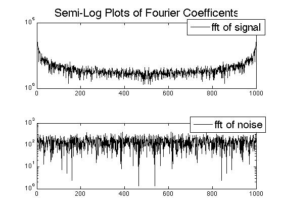

For instance, suppose is a random-walk and equals plus a considerable amount of noise,
where and are independent white noises, and . We should try to identify the bandwidth(s) that contain the support of ’s Fourier coefficients simply by looking at the support of the FFT of a random-walk and comparing it to the FFT of noise. From figure 7.1 we see that the dominant Fourier coefficients of a random-walk are either in an extremely high or an extremely low bandwidth, whereas the Fourier coefficients of the noise are evenly distributed across all bandwidths. If we take to be the high and low frequencies that only contain noise, then the reconstructed signal will have a higher SNR,
Indeed, as can be seen in figure 7.2, the signal becomes clearer as we eliminate the mid-level frequencies, and there is an increase in SNR from the 7.53 of the raw measurement, to 55.10 given by the bandwidth-filtered estimate, with a MSE=.0594.
7.1.3 Wavelet Filters
Wavelets are a tool that is useful in identifying the local behavior of a noise-corrupted signal. Measurements are often times contain adequate information for someone to decipher the underlying signal, usually because they can ignore noise and identify a movement in the measurement is caused by signal. This is precisely how a wavelet works: each wavelet represents a movement that the signal is capable of making, and any piece of the signal who’s cross-product resonates with the wavelet is removed and placed in its respective spot as part of a noiseless reconstruction of the underlying signal.
A wavelet basis consists of a set of self-similar functions
for integers and , where the unindexed function is the ‘mother-wavelet’. A useful wavelet has support that is small relative the length of the signal (e.g. ), and by construction should sum to zero and have norm 1,
with denoting the support of the wavelet. The wavelets are indexed by and where is a dilation and is a translation. The indices of the wavelets are chosen to form an orthonormal basis,
and like any other spectral method we can reconstruct a function from its wavelet transform,
for all , with denoting inner-product. Not all wavelets can be used to form an orthonormal basis (e.g. the Mexican hat), but such wavelets should not be considered useless. Rather, a wavelet without an orthonormal basis simply requires that one use methods other than spectral decomposition.
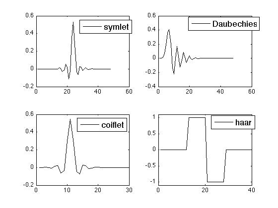
For a signal processing problem, a particular wavelet is chosen for its generic resemblance to a local behavior of which the signal is capable. Essentially, we are taking a convolution of the function with wavelets of different thickness , so that at each shift the local shape of the wavelet is given a chance to match itself to the input function. The wavelet-family that one uses will depend on the nature of the signal. Some possible wavelet to use in the construction of a discrete and orthogonal basis are symlets, coiflets, Daubechies, and Haar. The ‘mother wavelets’ for symlet24, a Daubechies24, a coiflet5, and a Haar, are shown in figure 7.3.
Symlet, coiflet and Daubechie wavelets can be defined with their respective degree of differentiability. For instance, a family of symlet-5 wavelets are generated by a mother-wavelet that has at least 6 derivatives and so three first 5 wavelet moments are vanishing,
for . In general, a wavelet that is -times differentiability with fast enough decay in its tails will -many vanishing moments.
When using wavelets to de-noise the random-walk example from section 7.1.2, there are numerous choices to make such as which wavelets to use and at what parameter values will we be fitting noise and not the signal. Figure 7.4 shows the wavelets’ ability to extract the signal from the noisy measurements, and table 7.1 shows how any of these wavelets does a better job de-noising the bandwidth filter from section 7.1.2.
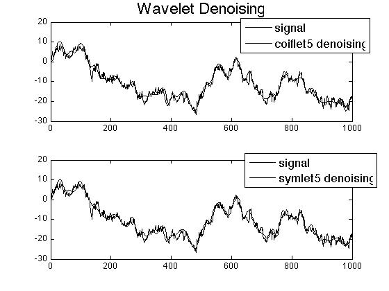
| wavelet | SNR | MSE |
| coif2 | 64.90 | 0.0549 |
| sym2 | 57.89 | 0.0581 |
| db2 | 57.89 | 0.0581 |
| coif5 | 59.32 | 0.0573 |
| sym5 | 58.38 | 0.0578 |
| db5 | 57.78 | 0.0581 |
| haar | 56.09 | 0.0589 |
7.2 Linear Gaussian Models
A special case is when the impulse response is a linear model with Gaussian noise,
where is the variance/covariance matrix of a mean-zero Gaussian noise. We give ourselves a greater ability to infer the state of the signal simply by assuming that the noise is Gaussian. In the simplest case, just knowing the covariance properties of the system is enough to make a projection onto a basis of orthogonal basis, a projection that may even be a posterior expectation if the model can be shown to have a jointly-Gaussian structure. If we further assume that the signal evolves according to an independent Gaussian model we can apply a Kalman filter, which is extremely effective for tracking hidden Markov processes, particularly ones of multiple dimension.
7.2.1 The Wiener Filter
Given the data , the signal combines with a noise so that
where , the covariance matrix of the noise is
and the covariance matrix of is
The information introduce by can be encapsulated in the innovation,
and the optimal linear estimate of is its projection,
where the matrix is defined apriori in such a way as to make the projection error orthogonal to the posterior information:
where we have assumed that because noise by construction should be independent of the signal. If we solve we get
| (7.1) |
which is the optimal projection matrix. The Wiener filter is essentially a linear projection using the matrix in (7.1). Notice that we have made minimal assumptions about the distributions of the random variables; all we have assumed is that we know the mean and covariance structure of and the driving noise in .
If we assume that are jointly Gaussian, then any random variable with the same distribution as is equal in distribution to a random variable that is a linear sum of and another Gaussian component that is independent of ,
where and are non-random matrices of coefficients, and is mean-zero Gaussian and independent of . With this representation we have
Now, by independence of and , we must have
which leads to the solution where is the projection matrix given by (7.1). In general, the MSE is bounded below by that of the posterior mean,
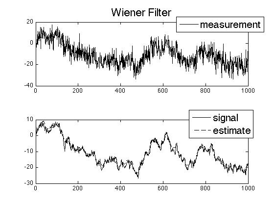
But if and are not jointly Gaussian, it can be shown that the MSE of the projection will be strictly greater than that of the posterior mean. In figure 7.5 the Wiener filter is used to track the random-walk example that was in section 7.1.2. For the random-walk example, the matrices are
which are ill-conditioned, but the round-off error is not significant for . Indeed, the SNR and MSE of the Wiener filter is 85.79 and .0479, both are better than the best results among the wavelet and bandwidth filters (the best was the coiflet with vanishing moments which had SNR = 64.90 and MSE = 0.0549). This example illustrates how the Wiener filter is the optimal among all posterior estimators.
Remark 4.
The resemblance of the Wiener filter to a penalized and weighted least-squares problem is clear from the first order conditions of the following minimization,
Remark 5.
When is a realization from a a jointly Gaussian HMM, the Wiener filter returns not only the posterior mean, but also the path of that is the maximum likelihood. In such cases, the estimator for can be consider a smoothing rather than a filtering because it is an estimate of the state’s past value,
Remark 6.
The numerical linear algebra for computing the Wienfer filter requires no inversion of matrices, but only to solve two linear systems. Observe, is the solution to a linear system,
so first we solve a linear system for
and then we solve for the filter,
7.2.2 The Kalman Filter
The Kalman filter can be thought of as a generalization of the Wiener filter, but for a model with a slightly more specific model for the signal. In fact, the Kalman filter is a filter for an HMM whose dynamics are Gaussian and fully linear,
where and are independent Gaussian random variables with covariance matrices
| (7.2) |
both of which are positive-definite, and the distribution of is a joint Gaussian. We can re-write this two equations as one linear system,
| (7.3) |
which is clearly a non-degenerate Gaussian system. In fact (7.3) has a stationary mean if the number is not included in the spectrum of .
Given the data , the Kalman filter will find the optimal projection of onto the Gaussian sub-space spanned by by iteratively refining the optimal projection of onto the space spanned by . Furthermore, the optimal projection will be equivalent to the posterior mean because are jointly Gaussian.
In this case we can identify a sequence of Gaussian random variables that are the innovations
but the idea is essentially the same as it was in the Wiener filter. Initially, letting we use a Wiener filter to get
where . Clearly, , and we can easily check that is jointly Gaussian, and so it follows that is independent of , and so posterior covariance is not a random variable,
Now we proceed inductively to identify the filter of given . Suppose we have obtain the filter up to time with posterior mean
for which is independent of , and with covariance matrix
When the observation arrives, the optimal projection will be
where is a projection matrix that is known at time ; it’s known before has been observed. We can verify that
-
•
the distribution of conditioned on is jointly Gaussian, and
-
•
that is independent of ,
and therefore it follows that . We can also write the following expression for the prediction covariance matrix,
and from the orthogonality of the projection residual to the data, we should have a projection matrix that satisfies the following equation,
We solve this equation to obtain the optimal projection matrix, also known as the Kalman filter Gain matrix
| (7.4) |
and using the gain matrix we can write the posterior mean as a recursive function of the innovation and the previous time’s posterior mean
| (7.5) |
Furthermore, we can verify that the conditional distribution of is jointly Gaussian, and since for all , it follows that is independent of . Therefore, the covariance matrix is not a function of the data
To summarize, we have shown that and independent of , and from equations (7.4), (7.5) along with the equations for and we have the Kalman filter at time
so that the posterior density of is
where is the dimension such that .
In figure 7.6 we see the Kalman filter’s ability to track the same random-walk example on which we test the filters from sections 7.1.2, 7.1.3 and 7.2.1.
The random-walk model is
and Kalman filter for the random-walk is
Given , the Kalman filter returns an optimal estimator of , not the entire path taken by . Indeed, the Kalman filter’s path has SNR = 43.88 and MSE = 0.0668, neither of which are better than the other filters. But this example should not be evidence for a dismissal of the Kalman filter, it simply shows that ex-ante estimation of the entire path of the signal is not its specialty.
The Kalman filter is far superior to the other filters we’ve discussed when it is applied to problems where is a multidimensional vector. When each observation is a vector, the curse of dimensionality makes it impossible to work with the basis’ required for bandwidth and wavelets, and the size of the matrices needed for the Wiener filter also be prohibitively large. On the other hand, the Kalman filter works efficiently and in real-time.
Remark 7.
For HMMs, the Kalman filter and the Wiener filter coincide in their estimates of the latest value of the signal,
Remark 8.
The Kalman filter is indeed capable of handling signals of high dimension, but there does not exist a general procedure for avoiding the explicit computation of the matrix inverse when computing the gain matrix. Sometimes this inverse may be manageable, but limitations in our ability to compute matrix inverse represent the upper-bound on the Kalman filter’s capacity.
Chapter 8 The Baum-Welch & Viterbi Algorithms
Filtering equations for the class of fully-discrete HMMs are relatively simple to derive through Bayesian manipulation of the posteriors. These discrete algorithms are interesting because they embody the most powerful elements of HMM theory in a very simple framework. The methods are readily-implementable and have become the workhorse in applied areas where machine learning algorithms are needed. The algorithms for filtering, smoothing and parameter estimation are analogous to their counterparts in continuous models, but the theoretical background required for understanding is minimal in the discrete setting.
8.1 Equations for Filtering, Smoothing & Prediction
Let denote a discrete time, and suppose that is an unobserved Markov chain taking values in a discrete state-space denoted by . Let denote ’s kernel of transition probabilities so that
for any , and .
Noisy measurements are taken in the form of a process which is a nonlinear function of , plus some noise,
where is an iid Gaussian random variable with mean zero and variance . The main feature of this discrete model is the memoryless-channel which allows the process to ‘forget the past’:
for any and for all .
8.1.1 Filtering
The filtering mass function is
for all . Through an application of Bayes rule along with the properties of the HMM, we are able to break down as follows,
where the memoryless-channel allows for the conditioning that occurs between the second and third lines. This recursive breakdown of the filtering mass is the forward Baum-Welch Equation, and can be written explicitly for the the system with Gaussian observation noise
| (8.1) |
where is a normalizing constant, and is a likelihood function
Equation (8.1) is convenient because it keeps the distribution updated without having to recompute old statistics as new data arrives. In ‘real-time’ it is efficient to use this algorithm to keep track of ’s latest movements, but older filtering estimates will not be optimal after new data has arrived. The smoothing distribution must be used to find the optimal estimate of at some time in the past.
8.1.2 Smoothing
For some time up to which data has been collected, the smoothing mass function is
Through an application of Bayes rule along with the properties of the model, the smoothing mass can be written as follows,
where is the normalizing constant from equation (8.1). Now suppose that we define a likelihood function for the events after time ,
for with the convention that . Then the smoothing mass can be written as the product of the filtering mass with
and from we can see that is given recursively by a backward Baum-Welch Equation
| (8.2) |
Clearly, computation of the smoothing distribution requires a computation of all filtering distribution up to time followed by the backward recursion to compute . In exchange for doing this extra work, the sequence of ’s estimates will suggest a path taken by that is more plausible than the path suggested by the filtering estimates.
8.1.3 Prediction
The prediction distribution is easier to compute than smoothing. For , the prediction distribution is
and is merely computed by extrapolating the filtering distribution,
where denotes the transition probability over time steps.
If is a positive recurrent Markov chain, then there is an invariant and the prediction distribution will converge to as . In some cases, the rate at which this convergence occurs will be proportional to the spectral gap in .
Suppose can take one of -many finite-state, and is a recurrent Markov chain with only 1 communication class. Let be the matrix of transition probabilities for , and suppose that so that
for all . Then the prediction distribution is
and will converge exponentially fast to the invariant measure with a rate proportional to the second eigenvalue of . To see why this is true, consider the basis of eigenvectors of , some of which may be generalized,
for some . Assuming that is the unique invariant mass function of , we have . By the Perron-Frobenius Theorem we can sort the eigenvalues so that , and we know that is a simple root of the characteristic polynomial and therefore is not a generalized eigenvector. From here we can see that
as . The spectral gap of is , and from the convergence rate we see that a greater spectral gap means that the prediction distribution will take less time to converge to the invariant measure. In general, the Perron-Frobenius theorem can be applied to a recurrent finite-state Markov chain provided that there is some integer for which for all .
8.2 Baum-Welch Algorithm for Learning Parameters
It is not very realistic to assume that we have apriori knowledge of the HMM that is completely accurate. However, stationarity of means that we are observed repeated behavior of , albeit through noisy measurements, but nevertheless we should be able to judge the frequencies with which occupies parts of the state-space and the frequencies with which it moves about.
If we have already computed the smoothing distribution based on a model that is ‘close’ in some sense, then we should have
| (8.3) | |||||
| (8.4) |
where is the stationary law of . With the Baum-Welch algorithm, we can in fact employ some optimization techniques to find a sequence of model estimates which are of increasing likelihood, and it turns out that the (8.3) and (8.4) are similar to the optimal improvement in selecting the sequence of models.
Consider two model parameters and . The Baum-Welch algorithm uses the Kullback-Leibler divergence to compare the two models,
If we set
we then have a simplified expression,
and rearranging the inequality we have
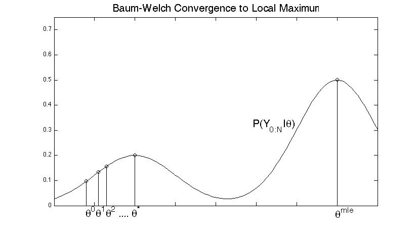
from which we see that implies that has greater likelihood than . The Baum-Welch algorithm uses this inequality as the basis for a criteria to iteratively refine the estimated model parameter. The algorithm obtains a sequence for which , and so their likelihoods are increasing but bounded,
where is the maximum likelihood estimate of . Therefore, will have a limit at such that
but it may be the case that (see figure 8.1).
In doing computations, a maximum (perhaps only a local maximum) of needs to be found. First-order conditions are good technique for finding one, and using the HMM we can expand into an explicit form,
| (8.5) |
from which we see that it is possible to differentiate with respect to , add the Lagrangians, and then solve for the optimal model estimate.
The Baum-Welch algorithm is equivalent to the expectation-maximization (EM) algorithm; the EM algorithm maximizes the expectation of the log-likelihood function which is equivalent to maximizing ,
8.2.1 Model Re-Estimation for Parametric Transition Probabilities
Suppose that , with transition probabilities parameterized by so that
where . Ignoring the parts that do not depend on , the log-likelihood is
and if we differentiate with respect to we have the following first-order conditions,
for any . The solution to the first-order conditions is that satisfies
for any .
8.2.2 Model Re-Estimation for Finite-State Markov Chains
Suppose , so that
for all . We will look for a sequence which maximizes subject to the constraints for all . Letting be the Lagrange multiplier for the th constraint, the first order conditions are then,
Multiplying by and summing over the expression in becomes
which means . By multiplying by and then rearranging terms it is found that the optimal must be chosen among the set of ’s such that
| (8.6) |
Now, using the expansion in (8.5), the derivative of with respect to can be computed as follows:
and by plugging this into equation (8.6) it is easily seen that the solution is
| (8.7) |
where . It also happens that equation (8.7) enforces non-negativity of , which is required for well-posedness of the algorithm. Equation (8.7) is equivalent to the estimates that were conjectured in (8.3) and (8.4).
8.3 The Viterbi Algorithm
Sometimes it may be more important to estimate the entire path of . The Viterbi algorithm applies the properties of the HMM along with dynamic programming to find an optimal sequence that maximizes the joint-posterior probability
Given the data , smoothing can be used to ‘look-back’ and make estimates of for some , but neither equations (8.1) or (8.2) is a joint posterior, meaning that they will not be able to tells us the posterior probability of a path . The size of our problem would grow exponentially with if we needed to compute the posterior distribution of paths, but the Viterbi algorithm allows us to obtain the MAP estimator of ’s path with without actually calculating the posterior probabilities of all paths.
The memoryless channel of the HMM allows us to write the maximization over paths as a nested maximization,
where is the likelihood and is the normalizing constant, both from the forward Baum-Welch equation in (8.1). To take advantage of this nested structure, it helps to define the following recursive function,
We then place is the nested structure of and work backwards to obtain the optimal path,
thus obtaining the optimal path in -many computations. It would have taken -many computations to obtain the posterior distribution of the paths.
We are interested in the Viterbi algorithm mainly because the path of estimates returned by the filtering and smoothing may
Remark 9.
The unnormalized probabilities in quickly fall below machine precision levels, so it is better to consider a logarithmic version of Viterbi,
and the use the ’s in the dynamic programming step,
Chapter 9 The Particle Filter
Monte Carlo methods have become the most common way to compute quantities from HMMs –and with good reason; they are in fact a fast and effective way to obtain consistent estimates. In particular, the particle filter is used to approximate filtering expectations. There are similar methods that exploit Bayes formula in obtaining samples from an HMM, but ‘particle filtering’ implies that sequential Monte Carlo (SIS) and Sampling-Importance-Resampling (SIR) are applied to the specified HMM.
9.1 The Particle Filter
Suppose that is an unobserved Markov chain taking values in a state-space denoted by . Let denote ’s kernel of transition densities so that
for any , and . Let the observed process be a nonlinear function of ,
where is an iid Gaussian random variable with mean zero and variance . In this case, the filter is easily shown to be a density function, given recursively as,
where is a normalizing constant, and is a likelihood function
but some kind quadrature grid would need to be established over if we were to use this recursive expression. An alternative is to use particles.
9.1.1 Sequential Importance Sampling (SIS)
Ideally, we would be able to sample directly from the filtering distribution to obtain a Monte Carlo estimate,
where . However, difficulties in computing also make it difficult to obtain samples. However, with relative ease we can sequentially obtain samples from unconditional distribution and then assign them weights in such a way that approximates the filter.
For , each particle is a path that is generated according to the unconditional distribution,
Then for -many particles and any integrable function , the strong law of large numbers tells us that
almost surely as .
Given , let denote the importance weight of a particle. We define to proportional to the likelihood of the th particle’s path, which we can write recursively as the product of its old weight and a likelihood function:
with the convention that , and is a normalizing constant
Then the filtering expectation of an integrable function can be consistently approximated with the weighted particles,
almost surely as by SLLN, where is a random variable with distribution and independent from .
9.1.2 Sampling Importance Resampling (SIR)
Our estimation of becomes a particle filter when SIR is used along with SIS. SIR essentially invokes a bootstrap on the samples at time . This procedure will reallocate our sampling resources onto particles that are more likely to be close to the true signal. When invoked, SIR does the following:
Algorithm 1.
SIR Bootstrap Procedure.
The common criterion for invoking SIR can be related to an entropy approximation of the particle distribution. At any time prior to when SIR has been performed, the entropy is defined as
and so maximizing the entropy of the particle distribution is approximately the same as minimizing the sum of squared posterior weights. Therefore, the criterion is to invoke SIR whenever the number of important particles is less than some threshold :
Even after SIR has been incorporated, our approximation is still consistent with the nonlinear filter:
Theorem 9.1.1.
For any bounded function ,
in as , and and are asymptotically independent for any .
Proof.
(taken from section 9.2 of [11]) Let be the set SIS samples that were in use prior to SIR. The post-SIR estimator can be written as a sum of the old samples:
where is the number of times the was resampled, . Taking conditional expectations, we have and the conditional expectation of the estimator is
From here we take expectations of both sides and use dominated convergence to equate the limit to show convergence,
as .
Now consider another bounded function ,
as . So we’ve found that
for and large. Therefore, and are asymptotically independent. ∎
Variance Reduction
For any bounded function , the principle of conditional Monte Carlo tells us that SIR estimator will have greater variance than the SIS estimator,
and so the estimator may not be preferable to . However, it follows from the proof of theorem 9.1.1 that
and we see a reduction in the overall variance of the particles if we write down the law of total variance,
This reduction can be quite significant if has a broad range. The rates are difficult to show, but by invoking SIR we obtain estimates of that will converge faster as . This brief subsection has not attempted any proof; we have not computed any comparison of convergence rates.
9.2 Examples
In this section we present some examples to demonstrate the particle filter’s uses.
9.2.1 Particle Fiter for Heston Model
Consider a Heston model with time-dependent coefficients
where is the log-price of an equity, is the volatility, is the correlation parameter , and are a pair of independent Wiener processes. The observed log-prices on equities and indices is not available in continuum. Instead, there is a discrete set sequence consisting of times at which quotes on the equity or index are given,
We denote the time step between the and observations . By considering the Stratonovich/Itô integral transform
and letting , we will find it useful to work with the following implicit discretization of the Stratonovich form of the Heston model,
where and are increments of independent Wiener processes (i.e. and ). We take to be the root of equation which can be obtained through the quadratic equation (see Alfonsi [2]),
Provided that and , this implicit scheme is effective because it is mean-reverting and preserves positivity in . With this scheme we can generate particles and approximate the nonlinear filter.
9.2.2 Rao-Blackwellization
Let be a hidden Markov chain with transition probabilities , and let be another hidden Markov process given by the following recursion,
with (to be clear, ), and Gaussian initial distribution . Let the observations process be defined discretely as
where are (to be clear and independent of ), and . In this case we can use particles to marginalize ,
and then for each particle we can compute the marginal Kalman filter,
where we have defined and (see [28, 25] for more on the Kalman Filter). Conditioned on , is normal with mean and variance
with the convention and . For any particle , the unnormalized importance weights are updated as follows:
with the convention that . For -many particles, the unnormalized Rao-Blackwellized filter is an approximation to the unnormalized filter,
where is a copy of that is independent of .
The Rao-Blackwell theorem says the following:
Theorem 9.2.1.
Rao-Blackwell. Given , let be an estimator of a parameter , and a sufficient statistic for . Then the estimator is at least as good in terms of MSE
for all in the parameter space.
Now, suppose that for each we generate particles instead of computing Kalman filters, and then using these particles we compute another estimator of the unnormalized filtering expectation,
But given , the marginal Kalman filter has allowed us to compute the likelihood without approximation. Therefore, a sufficient statistic for is , and we have
for all , and from here it is easy to see that the expectation of given is the Rao-Blackwellized estimator,
Therefore, by the Rao-Blackwell theorem we know that has less or equal MSE to a particle filter computed without marginal Kalman filters,
with the advantage that the Rao-Blackwellized filter requires particles to be simulated across a domain of fewer dimensions.
Chapter 10 Stability, Lyapunov Exponents, and Ergodic Theory for Finite-State Filters
A filter is said to be ‘stable’ if it has the ability to asymptotically recover from an erroneous initial distribution. In other words, assuming that all parts of the HMM are estimated correctly, but with the exception of the initial distribution which is incorrect, a stable filter will ‘forget’ the false assumptions as the initial data falls farther and farther into the past. It can be advantageous to work with a stable filter for a number of reasons, one being that parameter estimation algorithms for models with stable filters do not need to put as much emphasis on estimating the initial condition. Rates at which stability takes effect can also be estimated, as these rates are shown to be given by Lyapunov exponents or a spectral gap in the filter’s generator, and while the exponents are generally not explicitly computable, there are ways to make estimates. Finally, it is possible that a stable filter for an ergodic state variable may also have an ergodic theorem, a property that may be also be useful for parameter estimation.
10.1 Main Ideas and Their History
Consider an HMM where is a hidden Markov process taking values in a state-space with initial distribution , and where observations are made on the process which we assume to be given by a function of plus a noise. A filtering measure can be computed using the initial condition , and we denote it as
Definition 10.1.1.
Let be another probability measure on , and let denote the filter computed with as the initial distribution of . The filter is said to be asymptotically stable if
where denotes the total-variation norm.111The total variation norm of the difference between two probability measure and is where denotes the space of Borel-measurable subset of .
Intuitively, the filter should be stable if the model fits one of the following descriptions:
-
•
the signal is ergodic
-
•
or the observations are sufficiently informative, making old information obsolete (e.g. very low noise and is one-to-one),
but it is difficult to prove stability results even for these basic cases, and a general theory has yet to be developed.
Stability results for finite-state Markov chain signals are well-known along their rates, and their ergodic theory, and it has been known since the 1960’s that Kalman and Kalman-Bucy filters are stable when the signal is ergodic. The fundamental way of showing filter stability for these filters is to identify the equilibrium of the posterior covariance from its Ricatti equations, use it to show that the gain matrix also approaches an equilibrium, and then verify that the dependence on the initial condition fades with time. Example 10.1.1 shows how this is done for general Kalman-Bucy filters with constant coefficients, thus showing that observations in linear Gaussian models are indeed sufficiently informative since the signal is not assumed to be ergodic.
Example 10.1.1.
(Stability of Kalman-Bucy Filter with Constant Coefficients). Consider the following linear system,
where . Applying the Kalman-Bucy filter, we have
The solution to the Ricatti equation can be written explicitly as follows,
where
with . Asymptotically, we have and the filtering expectation is approximately,
where . This shows that the Kalman-Bucy filter will forget any initial condition on as , thus showing that the filter is stable.
General results for nonlinear filters with ergodic states were identified by Kunita in 1971 [31], but a key step in his proof is wrong. His proof essentially said the following:
Assume that . Then for any test function ,
where the denominator is strictly positive a.s. because . From this we see that the with Radon-Nykodym derivative
with -a.s. From the existence of the Radon-Nykodym derivative, the TV-norm is equivalent -a.s. to the following
| (10.1) |
but because of the Markov property, we realize that the distribution of given is the same regardless of whether information is added regarding the future. Therefore, we have
where denotes the tail--field generated by . Combining the tail--field measure with the numerator in (10.1) we have
and taking limits we have
which suggests that the filters are stable if and only if
| (10.2) |
To this point, every step is correct, but the error made by Kunita was in assuming that the limits of these filtrations were equal,
| (10.3) |
but there has since come a counter-example to equation (10.3).
10.1.1 The Counter Example
Baxendale, Chigansky and Lipster [8] presented an example to demonstrate when (10.3) fails. Let be a Markov chain taking values in with transition intensities
Clearly, all state communicate, and is an ergodic Markov process with invariant measure . Let , and consider the observations model
which is a degenerate noise model. The following lemma was proven in [8],
Lemma 10.1.1.
For this example, the limit of the filtrations in equation (10.3) is false,
Proof.
It suffices to show that is -measurable, but not measurable with respect to . The Markov chain only admits cycles in the following order,
and therefore we can recover given and for any (i.e. because we know we can look backwards and deduce the path of by looking at what times has jumped). Now, because , we have
Next, denote the times at which jumps with the sequence ( is time of ’s jump). It is not hard to verify that is independent of and the the following filtrations are equal,
and so for any we have
Since this posterior holds for any , we must have
which means that . ∎
10.2 Stability for Markov Chain Models
In this section we present some of the results in the paper by Atar and Zeitouni [4]. In particular, we present their proof of the stability-rate for discrete-time filtering problems where the state variable is an ergodic finite-state Markov chain. Their paper also presents the analogous results for continuous time, as well as some other results regarding the low-noise case.
Consider a probability space and let denote time. Suppose that is an unobserved Markov chain taking values in a finite state-space . Let the matrix contain ’s transition probabilities so that
for any , and . Suppose further that is recurrent with invariant law such that
as . We assume that is ergodic, which can be the case if and only if is of primitive order (i.e. there exists such that for all and for all ). Let the observed process be a nonlinear function of ,
where is an iid Gaussian random variable with mean zero and variance . The filtering mass computed with as its initial condition is denoted with and is given recursively by
where is a normalizing constant (dependent on ), and is a diagonal matrix of likelihood functions
Stability in this case means that for any other measure , we have
as , where denotes the Euclidean norm on . The rate of convergence of this difference is described in terms of Lyapunov exponents
for all , where the limit holds in some strong sense (such as probability, mean-square, or almost-surely). However, it turns out that the Lyapunov exponent is almost-surely bounded by a deterministic constant, dependent only on model parameters such as .
Before moving on, we define the sequence of stochastic operators , and define the sequence unnormalized posterior distributions,
| (10.4) |
Clearly, , where denotes the Euclidean inner-product on , and .
10.2.1 Perron-Frobenius & Oseledec’s Theorems
In this section we introduce some general results from matrix theory. The theorems are their usage have heavy dependence on the algebraic concept of an‘exterior product.’ For now, we start with a basic theory that we can apply to the eigenvalues and eigenvectors of a Markov chain transition matrix:
Theorem 10.2.1.
(Perron-Frobenius). Assuming that the Markov chain transition matrix is irreducible and of primitive order. Then 1 is a simple eigenvalue of with all other eigenvalues have real-part with absolute value strictly less than one. Moreover, the unique right-eigenvector corresponding to can be multiplied by a constant to equal , so that . Furthermore, for any probability vector we have as .
Proof.
(see Ethier and Kurtz [23]).∎
In filtering, we apply a sequence of matrices which are not time-homogenous. Therefore, we need to consider a more general framework when considering eigenvalues and the space of eigenvectors for . The multiplicative ergodic theorem, also known as Oseledec’s theorem, will be useful, but before we present the theorem we need to define the following,
Definition 10.2.1.
An operator where , is a cocycle if
-
•
for all ,
-
•
.
where .
Letting with the convention that , we see that is a cocycle. Now, we are ready for Oseledec’s theorem:
Theorem 10.2.2.
(Oseledec’s Multiplicative Ergodic Theorem). Suppose both and are integrable for all , for all . Then for each we have
exists and can take up to -many values. For some , if are the -many different (random) limits, then there exist (random) subspaces such that the limit is if for .
Proof.
(see page 181 of [12]).∎
In Oseledec’s theorem, the exponentials are the eigenvalues of the matrix . If should be noted that when , the space spanned by the non-generalized eigenvectors of will be .
A piece of matrix theory that will be useful is the exterior product. The exterior product or wedge product maps an two vectors to the parallelogram that they form. For more than two vectors, the exterior product corresponds the shape analogous to the parallelogram in the dimension equal to the number of vectors (for instance, the exterior product of three vectors is a parallelepiped). For any two vectors , their exterior product is
where represents the canonical basis of . Some basic properties of the exterior product are
-
•
-
•
-
•
and with regard to the Lyapunov exponents from Oseledec’s theorem, we have
10.2.2 Lyapunov Exponents of the Filter
Continuing to let , we can now show that the rate of convergence is given by the spectral gap in :
Theorem 10.2.3.
Assuming that is an ergodic Markov chain, there exists a deterministic function of , namely , such that for any , we have
-a.s. In particular, , which is the spectral gap in the matrix .
Proof.
From the triangle inequality, we can assume W.L.O.G. that the initial distribution of is its invariant distribution, and take . In this case, the matrices possess a stationary law which is also ergodic. Moreover,
Hence, we can apply Oseledec’s theorem to conclude there exists a random subspace such that if then
| (10.5) |
-a.s. In this setting, are the Lyapunov exponents associated with the matrix . It is well-known that has a (random) limit a.s., the eigenvalues of which are . Note that is a non-negative matrix, thus by Perron-Frobenius theorem the eigenvector associated with the highest eigenvalue of has all entries real and non-negative. The last property thus holds for too, and hence for . Since must be orthogonal to the eigenvector associated with the highest eigenvalue of , if follows that cannot include any probability vector with all entries strictly positive. As cases where does not have all positive entries, notice that does for where was the constant such that for when . Thus, (10.5) holds for any probability measure .
Using Oseledec’s theorem again, this time for -valued process , there exists a (random) strict subspace such that is then
| (10.6) |
-a.s., and for we have
| (10.7) |
-a.s.
Then using the inequality where is the sine of the angle between vectors and (see lemma 10.2.1), and the fact that
we can conclude that
which completes the proof. ∎
The difference is a spectral gap and its negativity is sufficient for the stability of the filters. In their paper [4], Atar and Zeitouni proceed to prove that when for all , then there exists a constant such that
where does not depend on or . They go on to prove that
They also prove the following bounds for low-noise models,
| (10.8) | |||||
| (10.9) |
Finally, with regard to the ergodic theory, it was shown by Chigansky in 2006 [17] that the Markov-Feller process has a unique invariant measure , such that for any continuous ,
| (10.10) |
where is the -marginal of .
10.2.3 Proof of
Let denote the set of -dimensional distribution vectors. If then for all , and . Furthermore, we can easily verify with a Jensen inequality that where is the Euclidean norm on . An inequality that will be useful is presented in the following lemma:
Lemma 10.2.1.
For any , we have
| (10.11) |
where is the sine of the angle between vectors and .
Proof.
For , the lemma is trivial, so the proof will focus on the case when .
The set can be defined by a hyperplane which is a dimensional surface inscribed in the non-negative region of whose distance from the origin is exactly unity under the -norm. For any vector , its distance to is defined as
From Jensen’s inequality, we know that for all with equality iff for all , so for we have
where . From the law of sines, for any vectors with , the vectors and the hyperplane’s surface form a triangle, and so we have a law of sines
| (10.12) |
From (10.12) we easily obtain
which shows that and proves the lower-bound in (10.11).
To get the upper-bound requires significantly more preparation. For any , let denote the sine of ’s angle of incidence with . Obviously, , and for any the most acute angle that can make with a vector parallel to the hyperplane is its angle of incidence, which is its angle with the vector ,
With the angle of incidence in mind, we observe the following inequality,
| (10.13) |
for any . The first inequality in (10.13) follows from the angle of incidence, and the second inequality is seen to be true if one notices that , the sine of its angle of incidence must be greater than or equal to that of , because the hyperplane’s surface is flat and the most acute angle of incidence is formed by a vector that stretches the farthest, which happens to be any one that touches a corner of . If we apply (10.12) to the triangle formed from and any , we obtain
giving us . Using this along with (10.13), we have
and using (10.12) we have
which proves the upper-bound.
∎
Bibliography
- [1] Ait-Sahalia, Y. (1999) Transition Densities for Interest Rate and Other Derivatives, The Journal of Finance, 54(4), pp. 1361–1395.
- [2] A. Alfonsi, “On the Discretization of the CIR (and Bessel squared) Processes,” 2005.
- [3] S. Asmussen, P. Glynn, Stochastic Simulation: Algorithms and Analysis. Springer, 2007.
- [4] R. Atar, O. Zeitouni, “Lyapunov Exponents for Finite State Nonlinear Filtering,” SIAM Journal on Control and Optimization, Vol 35, No 1, pp 33-55, January 1997.
- [5] A. Bain, D. Crisan, “Fundamentals of Stochastic Filtering,” Springer 2009.
- [6] Y. Bar-Shalom, X. R. LI, Estimation and Tracking: Principles, Techniques and Software. Boston: Artech House, 1993.
- [7] L. Baum, T. Petrie, G. Soules, N. Weiss, “A Maximization Technique Occurring in the Statistical Analysis of Probabilistic Functions of Markov Chains,” The Annals of Mathematical Statistics, Vol. 41, No. 1 (Feb., 1970), pp. 164-171.
- [8] P. Baxendale, P. Chigansky, R. Lipster, “An Asymptotic Theorem for Filtering with Applications to Stability,” Systems & Control Letters Volume 55, Issue 11, November 2006, Pages 908-917.
- [9] T. Björk. Arbitrage Theory in Continuous Time. 2nd edition, Oxford Press, 2004.
- [10] B.Z. Bobrovsky, O. Zeitouni “On the joint nonlinear filtering-smoothing of diffusion processes”, Systems & Control Letters Volume 7, Issue 4, July 1986, Pages 317-321
- [11] O. Cappé, E. Moulines, T. Rydén, Inference in Hidden Markov Models. Springer 2005.
- [12] R. Carmona, J. Lacroix “Spectral Theory of Random Schrödinger Operators,” Birkhäuser, 1990.
- [13] P. Carr, R. Lee, “Realized Volatility and Variance: Options via Swaps” Risk, May 2007.
- [14] P. Carr, D. Madan. “Towards a Theory of Volatility Trading,” reprinted in Option Pricing, Interest Rates, and Risk Management by Musiella, Jouini, Cvitanic, 1998, pp 417–427, University Press.
- [15] P. Carr, L. Wu, “Variance Risk Premia,” March 2005.
- [16] P. Carr, L. Wu, “A Tale of Two Indices,” The Journal of Derivatives, Spring 2006.
- [17] P. Chigansky, “ An Ergodic Theorem for Filtering Stability with Applications to Stability,” Systems & Control Letters, Vol 55, No 11, November 2006, Pages 908-917.
- [18] P. Chigansky, R. Lipster. R. Van Handel, “Intrinsic Methods in Filter Stability,” in Oxford University Handbook of Nonlinear Filtering (D. Crisan and B. Rozovsky, eds.), Oxford University Press, to appear.
- [19] E. Derman, K. Demeterfi, M. Kamal, J. Zou, “More Than You Ever Wanted to Know About Volatility Swaps” Journal of Derivatives 6(4), 1999, pages 9-32.
- [20] Drăgulescu, A. and Yakovenko, V. (2002) Probability distribution of returns in the Heston model with stochastic volatility, Quantitative Finance, 2, pp. 443–453.
- [21] P. Dupuis, H. Kushner Numerical Methods for Stochastic Control Problems in Continuous Time, 2nd edition. Springer 2001.
- [22] R.J. Elliot, A.V. Swishchuk. “Pricing Options and Variance Swaps in Markov Modulated Brownian Markets,” Hidden Markov Models in Finance, International Series in Operations Research & Management Science, Vol. 104
- [23] Stewart N. Ethier, Thomas G. Kurtz, Markov Processes: Characterization and Convergence. Wiley, 1986.
-
[24]
J.-P. Fouque, G. Papanicolaou, and R. Sircar,
Derivatives in Financial Markets with Stochastic Volatility, Cambridge University Press, 2000. - [25] B.Fristedt, N. Jain, N. Krylov, Filtering and Prediction: A Primer. American Mathematical Society, 2007.
- [26] J. Gatheral, The Volatility Surface, A Practioner’s Guide. Wiley, 2006.
- [27] S. Howison, A. Rafailidis, H. Rasmussen, “On the pricing and hedging of volatility derivatives” Applied Mathematical Finance, Volume 11, Issue 4 December 2000 , pages 317 - 346.
- [28] A. Jazwinski Stochastic Processes and Filtering Theory. Dover 1970.
- [29] T. Kailath, A.H. Sayed, B. Hassibi, “Linear Estimation,” Prentice Hall, (2000).
- [30] I. Karatzas, S. Shreve, Brownian Motion and Stochastic Calculus (Graduate Texts in Mathematics) 2nd Edition, Springe 1992.
- [31] H.Kunita “Asymptotic Behavior of Nonlinear Filtering Errors of Markov Processes,” Journal of Multi-Variate Analysis, Vol 1. No 4, pp 365-393, 1971.
- [32] T.G. Kurtz, D.L. Ocone, “Unique Characterization of Conditional Distribution In Nonlinear Filtering,” Annals of Probability, 1988, Vol 16, No 1, pp 80-107.
- [33] H. Kushner “Numerical Approximation to Optimal Nonlinear Filters,” 2008, http://www.dam.brown.edu/lcds/publications/
- [34] Y.A. Kutoyants. Statistical Inference for Ergodic Diffusion Processes. Springer, London, 2004
- [35] S. Mallat, “A Wavelet Tour of Signal Processing,” 2nd ed. Academic Press (1999).
- [36] B. Øxendale, Stochastic Differential Equations: An Introduction with Applications, Springer 6th edition, 2007.
- [37] E. Pardoux, Filtrage Non Lineaire et Equations aux Derivees Partielles Stochastiques Associees. Ecole d’été de Probabilities de Saint-Fleur, 1989.
- [38] E. Platen, N. Bruti-Liberati, Numerical Solutions of Stochastic Differential Equations in Finance, Springer 2010.
- [39] Forsyth, David. Ponce, Jean.“Computer Vision – A modern approach”
- [40] L. R. Rabiner “A tutorial on Hidden Markov Models and selected applications in speech recognition”. Proceedings of the IEEE 77 (2), (February 1989). pages: 257-286.
- [41] B. Rozovsky, “On Infinite Dimensional Systems of Stochastic Differential Equations Arising in the Theory of Optimal Nonlinear Filtering,” Theory of Probability and its Applications, vol 17, no 1, 1972.
- [42] B. Rozovsky, “A simple proof of uniqueness for Kushner and Zakai equations” In Stochastic analysis, ed. E. Mayer-Wolf, 449-458. Boston: Academic Press, 1991.
- [43] B. Rozovsky, A. Petrov, “Optimal Nonlinear Filtering for Track-Before-Detect in IR Image Sequences.” SPIE proceedings: Signal and Data Processing of Small Targets, vol. 3809, Denver, Co, 1999.
- [44] B. L. Rozovskii, A. Petrov, R. B. Blazek, “Interacting Banks of Bayesian Matched Filters.” SPIE Proceedings: Signal and Data Processing of Small Targets, Vol. 4048, Orlando, FL, 2000.
- [45] Welch, Greg. Bishop, Gary. “An Introduction to the Kalman Filter,” Department of Computer Science, University of North Carolina at Chapel Hill
- [46] R. Whaley, “Derivatives on Market Volatility: Hedging Tools Long Overdue,” Journal of Derivatives, fall 1993.
- [47] G. George Yin, Qing Zhang, Continuous-Time Markov Chains and Applications: A Singular Perturbation Approach. Springer, 1998.