Nonparametric Independence Testing for
Small Sample Sizes
Abstract
This paper deals with the problem of nonparametric independence testing, a fundamental decision-theoretic problem that asks if two arbitrary (possibly multivariate) random variables are independent or not, a question that comes up in many fields like causality and neuroscience. While quantities like correlation of only test for (univariate) linear independence, natural alternatives like mutual information of are hard to estimate due to a serious curse of dimensionality. A recent approach, avoiding both issues, estimates norms of an operator in Reproducing Kernel Hilbert Spaces (RKHSs). Our main contribution is strong empirical evidence that by employing shrunk operators when the sample size is small, one can attain an improvement in power at low false positive rates. We analyze the effects of Stein shrinkage on a popular test statistic called HSIC (Hilbert-Schmidt Independence Criterion). Our observations provide insights into two recently proposed shrinkage estimators, SCOSE and FCOSE - we prove that SCOSE is (essentially) the optimal linear shrinkage method for estimating the true operator; however, the non-linearly shrunk FCOSE usually achieves greater improvements in test power. This work is important for more powerful nonparametric detection of subtle nonlinear dependencies for small samples.
1 Introduction
The problem of nonparametric independence testing deals with ascertaining if two random variables are independent or not, making no parametric assumptions about their underlying distributions. Formally, given samples for where , that are drawn from a joint distribution supported on , we want to decide between the null and alternate hypotheses
where are the marginals of w.r.t. . A test is a function from the data to . Tests aim to have high power (probability of detecting dependence, when it exists) at a prespecified allowable type-1 error rate (probability of detecting dependence when there isn’t any).
Independence testing is often a precursor to further analysis. Consider for instance conditional independence testing for inferring causality, say by the PC algorithm Spirtes et al. (2000), whose first step is (unconditional) independence testing. It is also useful for scientific discovery like in neuroscience, to see if a stimulus (say an image) is independent of the brain activity (say fMRI) in a relevant part of the brain. Since detecting nonlinear correlations is much easier than estimating a nonparametric regression function (of onto ), it can be done at smaller sample sizes, with further samples collected for estimation only if an effect is detected by the hypothesis test. For such situations, correlation only tests for univariate linear independence, while other statistics like mutual information that do characterize multivariate independence are hard to estimate from data, suffering from a serious curse of dimensionality. A recent popular approach for this problem (and a related two-sample testing problem) involve the use of quantities defined in reproducing kernel Hilbert spaces (RKHSs) - see Gretton et al. (2006); Harchaoui et al. (2007); Gretton, Herbrich, Smola, Bousquet & Schölkopf (2005); Gretton, Bousquet, Smola & Schölkopf (2005).
This paper will concern itself with increasing the statistical power at small samples of a popular kernel statistic called HSIC, by using shrunk empirical estimators of the unknown population quantity (introduced below).
1.1 Hilbert Schmidt Independence Criterion
Due to limited space, familiarity with RKHS terminology is assumed - see Scholkopf & Smola (2002) for an introduction. Let and be two positive-definite reproducing kernels that correspond to RKHSs and respectively with inner-products and . Let arise from (implicit) feature maps and . In other words, are not functions, but mappings to the Hilbert space. i.e. respectively. These functions, when evaluated at points in the original spaces, must satisfy and .
The mean embedding of and are defined as and whose empirical estimates are and . Finally, the cross-covariance operator of is defined as
where is an outer-product. For unfamiliar readers, if we used the linear kernel and , then the cross-covariance operator is just the cross-covariance matrix. The plug-in empirical estimator of is
For conciseness, define , , and . The test statistic Hilbert-Schmidt Independence Criterion (HSIC) defined in Gretton, Bousquet, Smola & Schölkopf (2005) is the squared Hilbert-Schmidt norm of , and can be calculated using centered kernel matrices , where , as
| (1) |
For unfamiliar readers, if we used the linear kernel, this just corresponds to the Frobenius norm of the cross-covariance matrix. The most important property is: when the kernels are “characteristic”, then the corresponding population statistic is zero iff are independent Gretton, Bousquet, Smola & Schölkopf (2005). This gives rise to a natural test - calculate and reject the null if it is large.
Examples of characteristic kernels include Gaussian and Laplace , for any bandwidth , while the aforementioned linear kernel is not characteristic — the corresponding HSIC tests only linear relationships, and a zero cross-covariance matrix characterizes independence only for multivariate Gaussian distributions. Working with the infinite dimensional operator with characteristic kernels, allows us to identify any general nonlinear dependence (in the limit) between any pair of distributions, not just Gaussians.
1.2 Independence Testing using HSIC
A permutation-based test is described in Gretton, Bousquet, Smola & Schölkopf (2005), and proceeds in the following manner. From the given data, calculate the test statistic . Keeping the order of fixed, randomly permute a large number of times, and recompute the permuted HSIC each time. This destroyed any dependence between simulating a draw from the product of marginals, making the empirical distribution of the permuted HSICs behave like the null distribution of the test statistic (distribution of HSIC when is true). For a pre-specified type-1 error , calculate threshold in the right tail of the null distribution. Reject if . This test was proved to be consistent against any fixed alternative, meaning for any fixed type-1 error , the power goes to 1 as . Empirically, the power can be calculated using simulations by repeating the above permutation test many times for a fixed (for which dependence holds), and reporting the empirical probability of rejecting the null (detecting the dependence). Note that the power depends on (unknown to the user of the test).
1.3 Shrunk Estimators of
Even though is an unbiased estimator of , it typically has high variance at low sample sizes. The idea of Stein shrinkage Stein (1956) is to trade-off bias and variance, first introduced in the context of Gaussian mean estimation. This strategy of introducing some bias and decreasing the variance to get different estimators of was followed by Muandet et al. (2014) who define a linear shrinkage estimator of called SCOSE (Simple Covariance Shrinkage Estimator) and a nonlinear shrinkage estimator called FCOSE (Flexible Covariance Shrinkage Estimator). When we refer to shrunk estimators, we implicitly mean SCOSE and FCOSE. We will describe these briefly in Section 2.
1.4 Contributions
Our first contribution is the following :
1. We provide evidence that employing shrunk estimators of , instead of , to calculate the aforementioned test statistic, can increase the power of the associated independence test at low false positive rates, when the sample size is small (there is higher variance in estimating infinite-dimensional operators).
Our second contribution is to analyze the effect of shrinkage on the test statistic, to provide some practical insight.
2. The effect of shrinkage on the test-statistic is very similar to soft-thresholding (see Section 4), shrinking very small statistics to zero, and shrinking other values nearly (but not) linearly, and nearly (but not) monotonically.
Our last contribution is an insight on the two estimators considered in this paper, SCOSE and FCOSE.
3. We prove that SCOSE is (essentially, up to lower order terms) the optimal/oracle linear shrinkage estimator with respect to quadratic risk (see Section 5). However, we observe that FCOSE typically achieves higher power than SCOSE. This indicates that it may be useful to search for the optimal estimator in a larger class than linearly shrunk estimators, and also that quadratic loss may not be the right loss function for the purposes of test power.
The rest of this paper is organized as follows. Section 2 introduces SCOSE, FCOSE and their corresponding shrunk test statistics. Section 3 presents illuminating experiments that bring out the statistically significant improvement in power over HSIC. Section 4 conducts a deeper investigation into the effect of shrinkage and proves the oracle optimality of SCOSE under quadratic risk.
2 Shrunk Estimators and Test Statistics
Let represent the set of Hilbert-Schmidt operators from to . We first note that can be written as the solution to the following optimization problem.
Using this idea Muandet et al. (2014) suggest the following two shrunk/regularized estimators.
From SCOSE to
This is derived in Muandet et al. (2014) by solving
and the optimal solution (called SCOSE) is
where (and hence the shrinkage intensity) is estimated by leave-one-out cross-validation (LOOCV), in closed form as
Observing the expression for in Muandet et al. (2014), the denominator can be negative (for example, with the Gaussian kernel for small bandwidths, resulting in a kernel matrix close to the identity). This can cause to be negative, and to be (unintentionally) outside the range . Though not discussed in Muandet et al. (2014), we shall follow the convention that when , we shall use and if , we use . Indeed, one can show that dominates where . In Section 4, we prove that is (essentially) the optimal/oracle linear shrinkage estimator with respect to quadratic risk.
We can now calculate the corresponding shrunk statistic
| (2) |
While the above expression looks daunting, one thing to note is that the amount that HSIC is shrunk (i.e. the multiplicative factor) depends on the value of HSIC. As we shall see in section 4, small HSIC values get shrunk to zero, but as can be seen above, the shrinkage of HSIC is non-monotonic.
From FCOSE to
The Flexible Covariance Shrinkage Estimator is derived by relying on the Representer theorem, see Scholkopf & Smola (2002), to instead minimize
over all , and the optimal solution (called FCOSE) is
where denotes elementwise (Hadamard) product, is the vector , and as before the best is determined by LOOCV. The procedure to evaluate the optimal efficiently is described by Muandet et al. (2014) - a single eigenvalue decomposition of costing can be done, following which evaluating LOOCV is only per , see Muandet et al. (2014), section 3.1 for more details. As before, after picking the by LOOCV, we can derive the corresponding shrunk test statistic as
where . Note here that the shrinkage is not linear, and the effect on HSIC cannot be seen immediately. Similar to SCOSE, we shall see in section 4, small HSIC values get shrunk to zero (LOOCV chooses a large ).
3 Linear Shrinkage and Quadratic Risk
In this section, we prove that SCOSE is (essentially) optimal within a particular class of estimators. Such “oracle” arguments also exist elsewhere in the literature, like Ledoit & Wolf (2004), so we provide only a brief proof outline.
Proposition 1.
The oracle (with respect to quadratic risk) linear shrinkage estimator and intensity is defined as
and is given by where
Proof.
Define , , . Since , it is easy to verify that . Substituting and expanding the objective, we get:
Differentiating and equating to zero, gives . ∎
This appears in terms of quantities that depend on the unknown underlying distribution (hence the term oracle estimator). We use plugin estimates for . Let . Since is the variance of , let be the sample variance of , i.e. . Plugging these into and simplifying, we see that is
| (3) |
Comparing Eq.(3) with Eq.(2) shows that SCOSE is essentially , up to a factor in the denominator which is of the same order as the bias of the HSIC empirical estimator222HSIC and both converge to population HSIC at same rate determined by the dominant term (HSIC). (see Theorem 1 in Gretton, Bousquet, Smola & Schölkopf (2005)). In other words, SCOSE just corresponds to using a slightly different estimator for than the simple plugin , which varies on the same order as the bias . Hence SCOSE, as estimated via regularization and LOOCV, is (essentially) the optimal linear shrinkage estimator under quadratic risk.
To the best of our knowledge, this is the first such characterization of optimality of an estimator achieved through leave-one-out cross-validation. We are only able to prove this because one can explicitly calculate both the oracle linear shrinkage intensity as well as the optimal (as mentioned in Section 2). This raises a natural open question — can we find other situations where the LOOCV estimator is optimal with respect to some risk measure? (perhaps when explicit calculations are not possible, like ridge regression).
4 Experiments
In this section, we run three kinds of experiments: a) to verify that SCOSE has better quadratic risk than FCOSE and original sample estimator, b) detailed synthetic experiments to verify that shrinkage does improve power, across interesting regimes of , and c) real data obtained from MNIST, to show that we shrinkage detect dependence at much lower samples than the original data size.
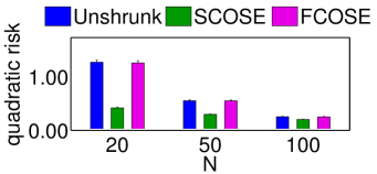
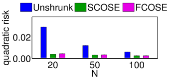
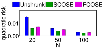
4.1 Quadratic Risk
Figure 1 shows that SCOSE is indeed much better than both and FCOSE with respect to quadratic risk. Here, we calculate for the distribution given in dataset (A) for . The expectation is calculated by repeating the experiment 1000 times. Each time is calculated according to samples and is approximated by the empirical cross-covariance matrix on 5,000 samples. The four panels use four different kernels which are linear, polynomial, Laplace and Gaussian from top to bottom. The shrunk estimators are always better than the unshrunk, with a larger difference between SCOSE and FCOSE for finite-dimensional feature spaces (top two). In infinite-dimensional feature spaces (bottom two), SCOSE and FCOSE are much better than the unshrunk estimator but very similar to each other. The differences between all estimators decreases with increasing , since the sample cross-covariance operator itself becomes very accurate.

4.2 Synthetic Data
We perform synthetic experiments in a wide variety of settings to demonstrate that the shrunk test statistics achieve higher power than HSIC in a variety of settings. We follow the schema provided in the introduction for independence testing and calculating power. We only consider difficult distributions with nonlinear dependence between , on which linear methods like correlation are shown to fail to detect dependence (some of them were used in previous papers on independence testing like Gretton et al. (2007) and Chwialkowski & Gretton (2014)).
For all experiments, is chosen as the type-1 error (for choosing the threshold level of the null distribution’s right tail). For every setting of parameters of each experiment, power is calculated as the percentage of rejection over 200 repetitions (independent trials), with 2000 permutations per repetition (permutation testing to find the null distribution threshold at level ). We use the Gaussian kernel where the bandwidth is chosen by the common median heuristic Scholkopf & Smola (2002).
Table 1 is a representative sample from what we saw on other examples - either large, small or no improvement in power was seen but almost never a worsening of power. The improvements in power may not always be huge, but they are statistically significant - it is difficult to detect such non-linear dependencies at low sample sizes, so any increase in power can be important in scientific applications.
Remark. A more appropriate way than using error bars to assess significance is by the Wilcoxon rank sum test, omitted for lack of space, though it yields more favorable results.
4.3 Real Data
We use two real datasets - the first is a good example where shrinkage helps a lot, but in the second it does not help (we show it on purpose). Like the synthetic datasets, for most real datasets it either helps or does not hurt (being very rarely worse; see remark in the discussion section).
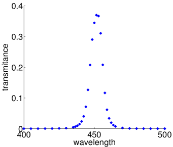
The first is the Eckerle dataset Eckerle (1979) from the NIST Statistical Reference Datasets (NIST StRD) for Nonlinear Regression, data from a NIST study of circular interference transmittance (n=35, is transmittance, is wavelength). A plot of the data in Figure 2 reveals a nonlinear relationship between (though the correlation is 0.035 with p-value 0.84). We subsample the data to see how often we can detect a relationship at of the original data size, when the false positive level is always controlled at 0.05. The second is the Aircraft dataset Bowman & Azzalini (2014) (n=709, is log(speed), is log(span)). Once again, correlation is low, with a p-value of over 0.8, and we subsample the data to of the original data size.
| = 0.01 | = 0.05 | = 0.10 | |||||||||||||
| HSIC | HSIC | HSIC | |||||||||||||
![[Uncaptioned image]](/html/1406.1922/assets/x5.png)
|
0.22 0.03 | 0.21 0.03 | 0.34 0.03 | ✓ | 0.52 0.04 | 0.52 0.04 | 0.71 0.03 | ✓ | 0.73 0.03 | 0.72 0.03 | 0.90 0.02 | ✓ | |||
![[Uncaptioned image]](/html/1406.1922/assets/x6.png)
|
0.41 0.03 | 0.41 0.03 | 0.48 0.04 | ✓ | 0.68 0.03 | 0.68 0.03 | 0.88 0.02 | ✓ | 0.85 0.03 | 0.85 0.02 | 0.99 0.01 | ✓ | |||
![[Uncaptioned image]](/html/1406.1922/assets/x7.png)
|
0.41 0.03 | 0.40 0.03 | 0.52 0.04 | ✓ | 0.74 0.03 | 0.74 0.03 | 0.94 0.02 | ✓ | 0.94 0.02 | 0.94 0.02 | 0.99 0.01 | ✓ | |||
![[Uncaptioned image]](/html/1406.1922/assets/x8.png)
|
0.52 0.04 | 0.52 0.04 | 0.66 0.03 | ✓ | 0.91 0.02 | 0.91 0.02 | 0.89 0.02 | 0.99 0.01 | 0.99 0.01 | 0.96 0.01 | ✗ | ||||
![[Uncaptioned image]](/html/1406.1922/assets/x9.png)
|
0.04 0.01 | 0.04 0.01 | 0.04 0.01 | 0.12 0.02 | 0.12 0.02 | 0.14 0.02 | 0.23 0.03 | 0.23 0.03 | 0.24 0.03 | ||||||
![[Uncaptioned image]](/html/1406.1922/assets/x10.png)
|
0.10 0.02 | 0.10 0.02 | 0.12 0.02 | 0.31 0.03 | 0.31 0.03 | 0.40 0.03 | ✓ | 0.47 0.04 | 0.47 0.04 | 0.58 0.03 | ✓ | ||||
![[Uncaptioned image]](/html/1406.1922/assets/x11.png)
|
0.33 0.03 | 0.33 0.03 | 0.46 0.04 | ✓ | 0.77 0.03 | 0.77 0.03 | 0.91 0.02 | ✓ | 0.95 0.01 | 0.96 0.01 | 0.99 0.01 | ✓ | |||
![[Uncaptioned image]](/html/1406.1922/assets/x12.png)
|
0.93 0.02 | 0.93 0.02 | 0.96 0.01 | ✓ | 1.00 0.00 | 1.00 0.00 | 1.00 0.00 | 1.00 0.00 | 1.00 0.00 | 1.00 0.00 | |||||
![[Uncaptioned image]](/html/1406.1922/assets/x13.png)
|
0.07 0.02 | 0.07 0.02 | 0.09 0.02 | 0.24 0.03 | 0.26 0.03 | 0.32 0.03 | ✓ | 0.44 0.04 | 0.47 0.04 | 0.48 0.04 | |||||
![[Uncaptioned image]](/html/1406.1922/assets/x14.png)
|
0.06 0.02 | 0.07 0.02 | 0.09 0.02 | 0.26 0.03 | 0.28 0.03 | 0.32 0.03 | 0.45 0.04 | 0.47 0.04 | 0.48 0.04 | ||||||
![[Uncaptioned image]](/html/1406.1922/assets/x15.png)
|
0.10 0.02 | 0.12 0.02 | 0.14 0.02 | 0.34 0.03 | 0.34 0.03 | 0.39 0.03 | 0.51 0.04 | 0.52 0.04 | 0.53 0.04 | ||||||
![[Uncaptioned image]](/html/1406.1922/assets/x16.png)
|
0.07 0.02 | 0.07 0.02 | 0.10 0.02 | ✓ | 0.30 0.03 | 0.33 0.03 | 0.35 0.03 | 0.53 0.04 | 0.54 0.04 | 0.57 0.04 | |||||
![[Uncaptioned image]](/html/1406.1922/assets/x17.png)
|
0.04 0.01 | 0.05 0.02 | 0.04 0.01 | 0.18 0.03 | 0.27 0.03 | 0.24 0.03 | ✓ | ✓ | 0.34 0.03 | 0.45 0.04 | 0.44 0.04 | ✓ | ✓ | ||
![[Uncaptioned image]](/html/1406.1922/assets/x18.png)
|
0.16 0.03 | 0.20 0.03 | 0.20 0.03 | 0.45 0.04 | 0.58 0.03 | 0.58 0.03 | ✓ | ✓ | 0.67 0.03 | 0.73 0.03 | 0.73 0.03 | ✓ | ✓ | ||
![[Uncaptioned image]](/html/1406.1922/assets/x19.png)
|
0.34 0.03 | 0.43 0.04 | 0.43 0.04 | ✓ | ✓ | 0.71 0.03 | 0.80 0.03 | 0.79 0.03 | ✓ | ✓ | 0.85 0.03 | 0.90 0.02 | 0.89 0.02 | ✓ | |
![[Uncaptioned image]](/html/1406.1922/assets/x20.png)
|
0.63 0.03 | 0.72 0.03 | 0.73 0.03 | ✓ | ✓ | 0.91 0.02 | 0.92 0.02 | 0.92 0.02 | 0.95 0.01 | 0.96 0.01 | 0.96 0.01 | ||||


5 Discussion
Why might shrinkage improve power? Let us examine the net effect of using shrunk estimators on the value of HSIC, i.e. let us compare and to HSIC by computing these over all the repetitions of the permutation testing procedure described in the introduction. In Fig. 3, both estimators are visually similar in transforming the actual test statistic. Perhaps the more interesting phenomenon is that Fig. 3 is reminiscent of the graph of a soft-thresholding operator . Intuitively, if the unshrunk HSIC value is small, the shrinkage methods deem it to be “noise” and it is shrunk to zero. Looking at the X-axis scaling of the top and bottom row, the size of the region that gets shrunk to zero decreases with - as expected, shrinkage has less effect when has low variance). The shrinkage being non-monotone (more so for than in Figure 3) is key to achieving an improvement in power.
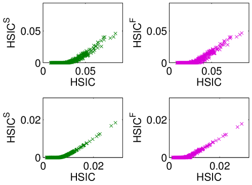
Using the intuition from the above figure, we can finally piece together why shrinkage may yield benefits. A rejection of occurs when the test statistic stands out in the right tail of its null distribution. Typically, when the alternative is true (this is when rejecting the null improves power) the unshrunk test statistics calculated from the permuted samples is smaller than the unshrunk HSIC calculated on the original sample. However, the effect of shrinking the small statistics towards zero, and setting the smallest ones to zero, is that the unpermuted test statistic under the alternative distribution stands out more in the right tail of the null.
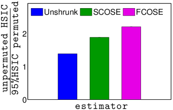
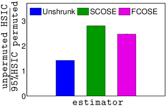
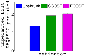
In other words, relative to the unshrunk null distribution and the unshrunk test statistic, the tail of the null distribution is shrunk more towards zero than the unpermuted test statistic, causing the latter to have a higher quantile in the right tail of the former (relative to the quantile before shrinkage). Let us verify this experimentally. In Fig.4 we plot for each of the datasets in Table 1, the average ratio of unpermuted statistic T to the 95th percentile of the permuted statistics, for . Recall that for dataset (C), we didn’t see much of an improvement in power, but for (A),(B),(D) it is clear from Fig. 4 that the unpermuted statistic is shrunk less than its null distribution’s 95th quantile.

Remark. In our experiments, real and synthetic, shrinkage usually improves (and almost never worsens) power in false-positive regimes that we usually care about. Will shrinkage always improve power? Possibly not. Even though shrunk the shrunk dominates for estimation error, it may not be the case that shrunk HSIC always dominates unshrunk HSIC for test power (i.e. the latter may not be inadmissible). However, just as no single classifier always outperforms another, it is still beneficial to add techniques like shrinkage, that seem to consistently yield benefits in practice, to the practitioner’s array of tools.
6 Conclusion
We presented evidence for an important phenomenon - using biased but lower variance shrunk estimators of cross-covariance operators can often significantly improve test power of HSIC at small sample sizes. This observation (that shrinkage can improve power) has rarely been made in the statistics and machine learning testing literature. We think the reason is that most test statistics for independence testing cannot be immediately expressed as the norm of an empirical operator, making it less obvious how to apply shrinkage to improve their power at low sample sizes.
We also showed the optimality (among linear shrinkage estimators) of SCOSE, but observe that the nonlinear shrinkage of FCOSE usually yields higher power. To the best of our knowledge, there seems to be no current literature showing that the choice made by leave-one-out cross-validation (SCOSE) explicitly leads to an estimator that is ”optimal” in some sense (among linear shrinkage estimators). This may be because it is often not possible to explicitly calculate the form of the LOOCV estimator, nor the explicit form of the best linear shrinkage estimator, as can both be done in this simple setting.
Since even the best possible linear shrinkage estimator (as represented by SCOSE) is usually worse than FCOSE, this result indicates that in order to improve upon FCOSE, it will be necessary to further study the class of non-linear shrinkage estimators for our infinite dimensional operators, as done for finite dimensional covariance matrices in Ledoit & Wolf (2011) and other papers by the same authors.
We ended with a brief investigation into the effect of shrinkage on HSIC and why shrinkage may intuitively improve power. We think that our work will be important for more powerful nonparametric detection of subtle nonlinear dependencies at low sample sizes, a common problem in scientific applications.
Acknowledgments
We would like to thank Arthur Gretton and Jessica Chemali for useful feedback on an earlier draft of the paper, Larry Wasserman for pointing out some useful references, and Krikamol Muandet for sharing his code. AR was supported in part by ONR MURI grant N000140911052.
References
- (1)
- Bowman & Azzalini (2014) Bowman, A. W. & Azzalini, A. (2014), R package sm: nonparametric smoothing methods (version 2.2-5.4), University of Glasgow, UK and Università di Padova, Italia.
- Chwialkowski & Gretton (2014) Chwialkowski, K. & Gretton, A. (2014), A kernel independence test for random processes, in ‘Proceedings of The 31st International Conference on Machine Learning’, pp. 1422–1430.
- Eckerle (1979) Eckerle, K. (1979), ‘Circular interference transmittance study’, National Institute of Standards and Technology (NIST), US Department of Commerce, USA .
- Gretton et al. (2006) Gretton, A., Borgwardt, K. M., Rasch, M., Schölkopf, B. & Smola, A. J. (2006), A kernel method for the two-sample-problem, in ‘Neural Information Processing Systems’, pp. 513–520.
- Gretton, Bousquet, Smola & Schölkopf (2005) Gretton, A., Bousquet, O., Smola, A. & Schölkopf, B. (2005), Measuring statistical dependence with Hilbert-Schmidt norms, in ‘Algorithmic Learning Theory’, Springer, pp. 63–77.
- Gretton et al. (2007) Gretton, A., Fukumizu, K., Teo, C. H., Song, L., Schölkopf, B. & Smola, A. J. (2007), ‘A kernel statistical test of independence’, Neural Information Processing Systems .
- Gretton, Herbrich, Smola, Bousquet & Schölkopf (2005) Gretton, A., Herbrich, R., Smola, A., Bousquet, O. & Schölkopf, B. (2005), ‘Kernel methods for measuring independence’, The Journal of Machine Learning Research 6, 2075–2129.
- Harchaoui et al. (2007) Harchaoui, Z., Bach, F. & Moulines, E. (2007), ‘Testing for homogeneity with kernel fisher discriminant analysis’, Arxiv preprint 0804.1026 .
- Ledoit & Wolf (2004) Ledoit, O. & Wolf, M. (2004), ‘A well-conditioned estimator for large-dimensional covariance matrices’, Journal of Multivariate Analysis 88(2), 365–411.
- Ledoit & Wolf (2011) Ledoit, O. & Wolf, M. (2011), ‘Nonlinear shrinkage estimation of large-dimensional covariance matrices’, Institute for Empirical Research in Economics University of Zurich Working Paper (515).
- Muandet et al. (2014) Muandet, K., Fukumizu, K., Sriperumbudur, B., Gretton, A. & Schoelkopf, B. (2014), Kernel mean estimation and stein effect, in ‘Proceedings of The 31st International Conference on Machine Learning’, pp. 10–18.
- Scholkopf & Smola (2002) Scholkopf, B. & Smola, A. (2002), Learning with kernels, MIT press Cambridge.
- Spirtes et al. (2000) Spirtes, P., Glymour, C. N. & Scheines, R. (2000), Causation, prediction, and search, Vol. 81, MIT press.
- Stein (1956) Stein, C. (1956), ‘Inadmissibility of the usual estimator for the mean of a multivariate normal distribution’, Proceedings of the Third Berkeley symposium on mathematical statistics and probability 1(399), 197–206.