Torsional Alfvén waves and the period ratio $P_{1}/P_{2}$ in spicules

Abstract

The effects of both density stratification and magnetic field expansion on torsional Alfvén waves in solar spicules are studied. Also, their eigenfrequencies, eigenfunctions, and the period ratio $P_{1}/P_{2}$ are obtained with a novel mathematical method. We showed that under some circumstances this ratio can approach its observational value even though it departs from its canonical value of $2$. Moreover, Eigenfunction height variations show that the oscillations amplitude are increasing towards higher heights which is in agreement with the observations. This means that with a little increase in height, amplitude of oscillations expands due to the significant decrease in the density.

Keywords Sun: spicules $\cdot$ MHD waves: Torsional Alfvén waves $\cdot$ period ratio

1 Introduction

Observation of oscillations in solar spicules may be used as an indirect evidence of energy transport from the photosphere towards the corona. Transverse motion of spicule axis can be observed by both, spectroscopic and imaging observations. The periodic Doppler shift of spectral lines have been observed from ground based coronagraphs (Nikolsky & Sazanov, 1987; Kukhianidze et al., 2006; Zaqarashvili et al., 2007). But Doppler shift oscillations with period of $\sim\!\!5$ min also have been observed on the SOlar and Heliospheric Observatory (SOHO) by Xia et al. (2005). Direct periodic displacement of spicule axes have been found by imaging observations on Solar Optical Telescope (SOT) on Hinode (De Pontieu et al., 2007; Kim et al., 2008; He et al., 2009).

The observed transverse oscillations of spicule axes were interpreted by kink (Nikolsky & Sazanov, 1987; Kukhianidze et al., 2006; Zaqarashvili et al., 2007; Kim et al., 2008; Ebadi et al., 2012a) and Alfvén (De Pontieu et al., 2007) waves. The kink mode, amongst others, differs from the torsional Alfvén mode, in that it displaces the whole flux tube in the transverse direction, while torsional mode does not displace the tube at all. Hence the kink mode is a bulk motion of the internal and external plasma, whereas the torsional Alfvén mode can exist independently on each magnetic surface. However, despite this significant difference, the kink mode is still highly Alfvénic (Verth et al., 2010). All spicule oscillations events are summarized in a recent review by Zaqarashvili & Erdélyi (2009).

One of the most important functions of coronal seismology is determining the period ratio $P_{1}/P_{2}$ between the period $P_{1}$ of the fundamental mode and the period $P_{2}$ of its first harmonic. Ebadi & Khoshrang (2014) analyzed the time series of oxygen line profiles, obtained from SUMER/SOHO on the solar south limb spicules. They calculated Doppler shifts and consequently Doppler velocities on a coronal hole region. They performed wavelet analysis to determine the periods of fundamental mode and its first harmonic mode. The calculated period ratios have departures from its canonical value of $2$. Different factors such as the effect of density stratification (Andries et al., 2009) and magnetic twist (Karami & Bahari, 2009, 2012) can cause the deviation of the period ratio from its canonical value.

The waves and the period ratio $P_{1}/P_{2}$ have been studied in coronal loops both theoretically and observationally. The observed values of this ratio in coronal loops is either smaller or larger than $2$ (Verwichte et al., 2004; Andries et al., 2009). Srivastava et al. (2008) Using simultaneous high spatial and temporal resolution H$\alpha$ observations studied the oscillations in the relative intensity to explore the possibility of sausage oscillations in the chromospheric cool post-flare loop. They used the standard wavelet tool, and find $P_{1}/P_{2}\sim 1.68$. They suggested that the oscillations represent the fundamental and the first harmonics of the fast-sausage waves in the cool post-flare loop. Orza et al. (2012) studied the $P_{1}/P_{2}$ period ratio of transversal loop oscillations for the diagnostics of longitudinal structuring of coronal loops. Their analysis shows that this ratio is sensitive to the temperature difference between the loop and its environment and this effect should always be taken into account when estimating the degree of density structuring. Verth et al. (2010) investigated how the radial and longitudinal plasma structuring affects the observational properties of torsional Alfvén waves in magnetic flux tubes. They showed that these waves are the ideal magnetoseismological tool for probing radial plasma inhomogeneity in solar waveguides. Karami & Bahari (2011) studied the effects of both density stratification and magnetic field expansion on torsional Alfvén waves in coronal loops. They concluded that the density stratification and magnetic field expansion have opposite effects on the oscillating properties of torsional Alfvén waves.

In the present work, we study the torsional Alfvén waves, and determine the period ratio $P_{1}/P_{2}$ and eigenfunctions in solar spicules.

2 Theoretical modeling

We consider an equilibrium configuration in the form of an expanding straight magnetic flux tube with varying density along tube. We use cylindrical coordinates $r$, $\varphi$, and $z$ with the $z$-axis coinciding along tube axis. Okamoto & De Pontieu (2011) claim that about $20\%$ of observed spicule kink waves are standing. Possibly there is a similar percentage of standing torsional Alfvén waves in spicules. So, in what follows we continue on standing torsional Alfvén waves with the nodes located at $z=0$ and $z=L$ ($L$ is spicule length).

To describe the plasma motion we use the linear ideal MHD equations for a cold plasma,

$$\frac{\partial^{2}\mathbf{\xi}}{\partial t^{2}}=\frac{1}{\mu_{0}\rho}(\nabla\times\mathbf{b})\times\mathbf{B},$$ (1)

and

$$\mathbf{b}=\nabla\times(\mathbf{\xi}\times\mathbf{B}),$$ (2)

where $\mathbf{\xi}=(0,\xi_{\varphi},0)$ is the plasma displacement, and $\mathbf{b}=(0,b_{\varphi},0)$ is the magnetic field perturbation. Rewriting Eqs 1, 2 in components and considering the time-dependence as $e^{-i\omega t}$ yields:

$$\mu_{0}\rho\omega^{2}\xi_{\varphi}+\frac{B_{r}}{r}\frac{\partial(rb_{\varphi})}{\partial r}+B_{z}\frac{\partial b_{\varphi}}{\partial z}=0,$$ (3)

and

$$b_{\varphi}=\frac{\partial(B_{r}\xi_{\varphi})}{\partial r}+\frac{\partial(B_{z}\xi_{\varphi})}{\partial z}.$$ (4)

Now like Verth et al. (2010); Ruderman et al. (2008); Karami & Bahari (2011) we use non-orthogonal flux coordinate in which $\psi$ becomes an independent variable instead of $r$, i.e. $r=r(\psi,z)$. For an arbitrary function $f$ we have the following relations:

$$B_{r} = rB_{z}\frac{\partial f}{\partial\psi}$$

$$B_{z} = \frac{\partial f}{\partial z}-rB_{r}\frac{\partial f}{\partial\psi}.$$ (5)

When deriving these equations we assumed thin tube approximation (or long-wavelength limit), i.e. $R/L\ll 1$ ($R$ is the radius of expanding spicule). The equilibrium magnetic field has two components, $r$, $z$, and independent of $\varphi$, so that $B=B(r,z)$. It follows from solenoidal condition that $B$ can be expressed in terms of flux function $\psi$,

$$\frac{\partial f}{\partial r} = -\frac{1}{r}\frac{\partial\psi}{\partial z}$$

$$\frac{\partial f}{\partial z} = \frac{1}{r}\frac{\partial\psi}{\partial r}.$$ (6)

Differentiating the identities $\psi=\psi(r(\psi,z),z)$ and $r=r(\psi(r,z),z)$ with respect to $z$ and using equation 2 yields:

$$\frac{\partial r}{\partial z} = \frac{B_{r}}{B_{z}}$$

$$\frac{\partial r}{\partial\psi} = \frac{1}{rB_{z}}.$$ (7)

By using Eqs 2, along with the solenoidal condition, we can simplify Eqs 3, 4 to

$$\mu_{0}\rho\omega^{2}\xi_{\varphi}+\frac{B_{z}}{R}\frac{\partial(Rb_{\varphi})}{\partial z}=0,$$ (8)

and

$$b_{\varphi}=RB_{z}\frac{\partial}{\partial z}\left(\frac{\xi_{\varphi}}{R}\right).$$ (9)

Eqs 8, 9 can now be combined as

$$\mu_{0}\rho\omega^{2}\xi_{\varphi}+\frac{B_{z}}{R}\frac{\partial}{\partial z}\left[R^{2}B_{z}\frac{\partial}{\partial z}\left(\frac{\xi_{\varphi}}{R}\right)\right]=0.$$ (10)

It would be more realistic to use the background magnetic field, plasma density, and spicule radius inferred from the actual magnetoseismology of observation (Verth et al., 2011):

$$B_{z}(z) = B_{0}\exp(-z/H_{B})$$

$$\rho(z) = \rho_{0}\exp(-z/H_{\rho})$$

$$R(z) = R_{0}\exp(z/2H_{B}),$$ (11)

where $H_{B}$ and $H_{\rho}$ are magnetic and density scale heights, respectively. The latter follows from the conservation of magnetic flux. Using Eqs 2 in equation 10 results in

$$\frac{\partial^{2}\xi_{\varphi}}{\partial z^{2}}-\frac{1}{H_{B}}\frac{\partial\xi_{\varphi}}{\partial z}+\left(\frac{1}{4H^{2}_{B}}+4\pi^{2}\omega^{2}e^{-\alpha z}\right)\xi_{\varphi}=0,$$ (12)

where $\alpha\equiv\left(\frac{H_{B}-2H_{\rho}}{H_{\rho}H_{B}}\right)$. In this equation the lengths are normalized to spicule length ($L$), and frequencies to Alfvén frequency ($\omega_{A}\equiv\frac{V_{A}}{L}=0.06$ rad/s; $V_{A}=\frac{B_{0}}{\sqrt{\mu_{0}\rho_{0}}}=75$ km/s; $B_{0}=12$ G, $\rho_{0}=1.9\times 10^{-10}$ kg m^-3, $\mu_{0}=4\pi\times 10^{-7}$ T m A^-1, and $L=8000$ km). Magnetic and density scale heights are determined as $H_{B}=1816$ km and $H_{\rho}=752$ km by Verth et al. (2011).

3 Numerical results and Discussions

We solve equation 12 numerically by using differential transform method (DTM)(see appendix for detailed description of this method) to obtain both eigenfrequencies and eigenfunctions of standing torsional Alfvén waves in stratified and expanding solar spicules. We use the rigid boundary conditions and assume that $\xi_{\varphi}(0)=\xi_{\varphi}(L)=0$. In Figure 1 we plotted Torsional Alfvén modes frequencies and the period ratio $P_{1}/P_{2}$ between the period $P_{1}$ of the fundamental mode and the period $P_{2}$ of its first harmonic. Frequencies are increasing with an increase of $\alpha$. The ratio $P_{1}/P_{2}$ is decreasing with $\alpha$ and reaching to observed values around $\alpha=3$ $(H_{B}\simeq 3H_{\rho})$. The fundamental mode and its first harmonic period ratios have departures from its canonical value of $2$. It is distinguished by observations which were made by Ebadi & Khoshrang (2014) in solar spicules. Andries et al. (2009) showed that the frequencies of detected kink oscillation overtones are in particular sensitive to the density and the magnetic field expansion. Karami & Bahari (2009) showed that the frequencies and the damping rates of both the kink and fluting modes increase when the twist parameter increases. These two factors are studied in spicules both observationally and theoretically. Verth et al. (2011) based on SOT/Hinode observations determined the variation of magnetic field strength and plasma density along a spicule by seismology. They studied a kink wave propagating along a spicule by estimating the spatial change in phase speed and velocity amplitude as a novel approach. Suematsu et al. (2008); Tavabi et al. (2011) by using the SOT/Hinode observations reported twisted motions in spicules.

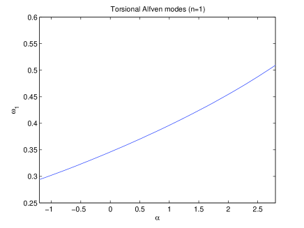
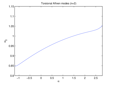
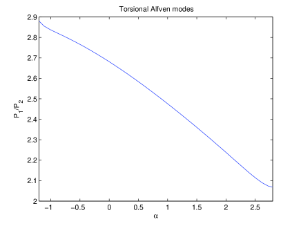
Fig. 1 : Torsional Alfvén modes frequencies and the period ratio $P_{1}/P_{2}$ between the period $P_{1}$ of the fundamental mode and the period $P_{2}$ of its first harmonic are plotted from top to down panels, respectively.

Eigenfunctions of the fundamental and first harmonic torsional Alfvén modes with respect to the normalized height along the spicule are presented in Figure 2. It should be emphasized that we plotted eigenfunctions for $\alpha=1.84$ which is determined by observations. It is interesting that the oscillations amplitude are increasing towards higher heights. The same behavior was observed in spicules by He et al. (2009); Ebadi et al. (2012a); Ebadi & Khoshrang (2014). This means that with a little increase in height, amplitude of oscillations become expanded due to significant decrease in density, which acts as inertia against oscillations.

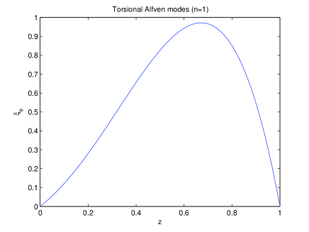
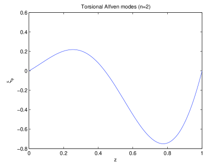
Fig. 2 : Eigenfunctions of the fundamental and first harmonic torsional Alfvén modes with respect to normalized height along the spicule are plotted in the first and second panels, respectively ($\alpha=1.84$).

4 Conclusion

We consider an equilibrium configuration in the form of an expanding straight magnetic flux tube with varying density along tube. We use cylindrical coordinates $r$, $\varphi$, and $z$ with the $z$-axis coinciding along tube axis. It is claimed that about $20\%$ of observed spicule waves, are standing torsional Alfvén waves. More realistic background magnetic field, plasma density, and spicule radios inferred from the actual magnetoseismology of observations are used. We used a novel mathematical method which was explained in the last section to solve equation 12. Fundamental and its first harmonic frequencies are increasing with $\alpha$. On the other hand their ratio is decreasing with $\alpha$ and reaching to the observed values around $\alpha\simeq 3$. The fundamental mode and its first harmonic period ratios have departures from its canonical value of $2$ which was distinguished by observations. The density stratification and magnetic twist are two main factors which make the period ratio departures from its canonical value of $2$. These two factors are studied in spicules both observationally and theoretically. Eigenfunction variations with height show that the oscillations amplitude are increasing towards higher heights. It is in agreement with the results of spicule observations. This means that with a little increase in height, amplitude of oscillations become expanded due to significant decrease in density, which acts as inertia against oscillations.

Acknowledgements This work has been supported financially by the Research Institute for Astronomy and Astrophysics of Maragha (RIAAM), Maragha, Iran.

5 Appendix

5.1 Differential Transform Method

The differential transform technique is one of the semi-numerical analytical methods for ordinary and partial differential equations that uses the polynomials as approximations of the exact solutions that are sufficiently differentiable (Erturk et al., 2012). The basic definition and fundamental theorems of the differential transform method (DTM) and its applicability for various kinds of differential and integral equations are given in Nzari & Shahmorad (2010); Tari & Shahmorad (2011); Ozkan (2010); Arikogli & OZKOL (2006). For convenience of the reader, we present a review of the DTM. The differential transform of the $k$th derivative of function $f(t)$ is defined as follows:

$$F(k)=\frac{1}{k!}\left[\frac{d^{k}f(t)}{dt^{k}}\right]_{t=t0},$$ (13)

where $f(t)$ is the original function and $F(k)$ is the transformed function. The differential inverse transform of $F(k)$ is defined as

$$f(t)=\sum_{k=0}^{\infty}F(k)(t-t_{0})^{k}.$$ (14)

From Eqs. 13 and 14, we get

$$f(t)=\sum_{k=0}^{\infty}\frac{(t-t_{0})^{k}}{k!}\frac{d^{k}f(t)}{dt^{k}}\|_{t=t0},$$ (15)

which implies that the concept of differential transform is derived from Taylor series expansion, but the method dose not evaluate the derivative symbolically. However, relative derivatives are calculated by an iterative way which are described by the transformed equations of the original function. For implementation purpose, the function $f(t)$ is expressed by a finite series and Equation 14 can be written as

$$f(t)=\sum_{k=0}^{N}F(k)(t-t_{0})^{k}.$$ (16)

Here $N$ is decided by the convergence of natural frequency. The fundamental operations performed by differential transform can readily be obtained and are listed in Table 1. The main steps of the DTM, as a tool for solving different classes of nonlinear problems, are the following. First, we apply the differential transform (Equation 13) to the given problem (integral equation, ordinary differential equation or partial differential equation), then the result is a recurrence relation. Second, solving this relation and using the differential inverse transform (Equation 16), we can obtain approximate solution of the problem.

Table 1: Operations of differential transform

$$\tiny{\begin{array}[]{cc}\hline\cr\text{Original function}&\text{Transformed function}\\ \hline\cr f(t)=u(t)\pm v(t)&F(k)=U(k)\pm V(k)\\ \hline\cr f(t)=u(t)v(t)&F(k)=\sum_{l=0}^{k}U(l)\times V(k-l)\\ \hline\cr f(t)=\alpha u(t)&F(k)=\alpha U(k)\\ \hline\cr f(t)=\frac{du(t)}{dt}&F(k)=(k+1)U(k+1)\\ \hline\cr f(t)=\frac{d^{m}u(t)}{{dt}^{m}}&F(k)=(k+1)(k+2)\cdots(k+m)U(k+m)\\ \hline\cr f(t)=\int_{t_{0}}^{t}u(t)dt&F(k)=\frac{U(k-1)}{k},\ \ k\geq 1\\ \hline\cr f(t)=t^{m}&F(k)=\delta(k-m)=\left\{\begin{array}[]{c}1,\ \ \ k=m,\\ 0,\ \ \ k\neq m.\end{array}\right.\\ \hline\cr f(t)=exp(\lambda,t)&F(k)=\frac{\lambda^{k}}{k!}\\ \hline\cr f(t)=sin(\omega t+\alpha)&F(k)=\frac{\omega^{k}}{k!}sin(\frac{\pi k}{2}+alpha)\\ \hline\cr f(t)=cos(\omega t+\alpha)&F(k)=\frac{\omega^{k}}{k!}cos(\frac{\pi k}{2}+alpha)\\ \hline\cr f(t)=\frac{u(t)}{v(t)}&F(k)=\frac{1}{V(0)}\left[U(k)-\sum_{m=0}^{k-1}U(k)V(k-m)\right]\\ \hline\cr f(t)={\left[u(t)\right]}^{b}&F(k)=\left\{\begin{array}[]{c}U(0),\ \ \ k=0,\\ \sum_{m=0}^{k}\frac{(b+1)m-k}{kU(0)}U(m)U(k-m),\ \ \ k\geq 1.\end{array}\right.\\ \hline\cr\end{array}}$$

References

- Andries et al. (2009) Andries, J., van Doorsselaere, T., Roberts, B., Verth, G., Verwichte, E., Erdélyi, R.: Space Sci. Rev. 149, 3 (2009)
- Arikogli & OZKOL (2006) Arikoglu, A., Ozkol, I.: Appl. Math. Comput. 173, 126 (2006).
- De Pontieu et al. (2007) De Pontieu, B., McIntosh, S.W., Carlsson, M., et al.: Science 318, 1574 (2007)
- Ebadi & Khoshrang (2014) Ebadi, H., Khoshrang, M.: Astrophys. Space Sci. Doi: 10.1007/s10509-014-1929-4 (2014)
- Ebadi et al. (2012a) Ebadi, H., Zaqarashvili, T.V., Zhelyazkov, I.: Astrophys. Space Sci. 337, 33 (2012a)
- Erturk et al. (2012) Erturk, V.S., Odibat, Z.M., Momani, S.: The Adv. Appl. Math. Mech., 4, 422 (2012).
- He et al. (2009) He, J., Marcsh, E., Tu, G., Tian, H.: Astrophys. J. Lett. 705, L217 (2009)
- Karami & Bahari (2012) Karami, K., Bahari, K.: Astrophys. J. 757, 186 (2012)
- Karami & Bahari (2011) Karami, K., Bahari, K.: Astrophys. Space Sci. 333, 463 (2011)
- Karami & Bahari (2009) Karami, K., Bahari, K.: Mon. Not. R. Astron. Soc. 394, 521 (2009)
- Kim et al. (2008) Kim, Y.H., Bong, S.C., Park, Y.D., Cho, K.S., Moon, Y.J., Suematsu, Y.: J. Korean Astron. Soc. 41, 173 (2008)
- Kukhianidze et al. (2006) Kukhianidze, V., Zaqarashvili, T.V., Khutsishvili, E.: Astron. Astrophys. 449, 35 (2006)
- Nzari & Shahmorad (2010) Nazari, D., Shahmorad, S.: J. Comp. Appl. Math., 234, , 883 (2010).
- Nikolsky & Sazanov (1987) Nikolsky, G.M., Sazanov, A.A.: Soviet Astron. 10, 744 (1967)
- Okamoto & De Pontieu (2011) Okamoto, T.J., De Pontieu, B.: Astrophys. J. 736, 24 (2011)
- Orza et al. (2012) Orza, B., Ballai, I., Jain, R., Murawski, K.: Astron. Astrophys. 537, 41 (2012)
- Ozkan (2010) Ozkan, O.: Int. J. Comput. Math., 87, 2786 (2010).
- Srivastava et al. (2008) Srivastava, A. K., Zaqarashvili, T. V., Uddin, W., Dwivedi, B. N., Kumar, Pankaj: Mon. Not. R. Astron. Soc. 388, 1899 (2008)
- Suematsu et al. (2008) Suematsu, Y., Ichimoto, K., Katsukawa, Y., Shimizu, T., Okamoto, T., Tsuneta, S., Tarbell, T., Shine, R. A.: ASP Conference Series, 397, 27 (2008)
- Verth et al. (2010) Verth, G., Erdélyi, R., Goossens, M.: Astrophys. J. 714, 1637 (2010)
- Ruderman et al. (2008) Ruderman, M.S., Verth, G., Erdélyi, R.: Astrophys. J. 686, 694 (2008)
- Tari & Shahmorad (2011) Tari A., Shahmorad, S.: Comput. Math. Appl., 61, 2621 (2011).
- Tavabi et al. (2011) Tavabi, E., Koutchmy, S., Ajabshirizadeh, A.: New Astron. 16, 296 (2011)
- Verth et al. (2011) Verth, G., Goossens, M., He, J.-S.: Astrophys. J. Lett. 733, 15 (2011)
- Verwichte et al. (2004) Verwichte, E., Nakariakov, V. M., Ofman, L., Deluca, E. E.: Sol. Phys. 223, 77 (2004)
- Xia et al. (2005) Xia, L.D., Popescu, M.D., Doyle, J.G., Giannikakis, J.: Astron. Astrophys. 438, 1152 (2005)
- Zaqarashvili & Erdélyi (2009) Zaqarashvili, T.V., Erdélyi, R.: Space Sci. Rev. 149, 335 (2009)
- Zaqarashvili et al. (2007) Zaqarashvili, T.V., Khutsishvili, E., Kukhianidze, V., Ramishvili, G.: Astron. Astrophys. 474, 627 (2007)