A Refined Holographic QCD Model and QCD Phase Structure

Abstract

We consider the Einstein-Maxwell-dilaton system with an arbitrary kinetic gauge function and a dilaton potential. A family of analytic solutions is obtained by the potential reconstruction method. We then study its holographic dual QCD model. The kinetic gauge function can be fixed by requesting the linear Regge spectrum of mesons. We calculate the free energy to obtain the phase diagram of the holographic QCD model.

I Introduction

To study phase structure of QCD is a challenging and important task. It is well known that QCD is in the confinement and chiral symmetry breaking phase at the low temperature and small chemical potential, while it is in the deconfinement and chiral symmetry restored phase at the high temperature and large chemical potential. Thus it is widely believed that there exists a phase transition between these two phases. To obtain the phase transition boundary in the $T-\mu$ phase diagram is a rather difficult task because the QCD coupling constant becomes very strong near the phase transition region and the conventional perturbative method does not work well. Moreover, with the nonzero physical quark masses presented, part of the phase transition line will weaken to a crossover for a range of temperature and chemical potential that makes the phase structure of QCD more complicated to study. Locating the critical point where the phase transition converts to a crossover is an important but difficult task. For a long time, the technique of lattice QCD is the only reliable method to attack these problems. Although lattice QCD works very well for zero density, it encounters the sign problem when considering finite density or chemical potential, i.e. $\mu\neq 0$. However, the most interesting region in the QCD phase diagram is at finite density. The most concerned subjects, such as heavy-ion collisions and compact stars in astrophysics, are all related to QCD at finite density. Recently, lattice QCD has developed some techniques to solve the sign problem, such as reweighting method, imaginary chemical potential method and the method of expansion in $\mu/T$. Nevertheless, these techniques are only able to deal with the cases of small chemical potentials and quickly lost control for the larger chemical potential. See 1009.4089 for a review of the current status of lattice QCD.

On the other hand, using the recently developed idea of AdS/CFT correspondence from string theory, one is able to study QCD in the strongly coupled region by studying its weakly coupled dual gravitational theory, the so called holographic QCD. The models which are directly constructed from string theory are called top-down models. The most popular top-down models are D3-D7 0306018 ; 0311270 ; 0304032 ; 0611099 model and D4-D8 (Sakai-Sugimoto) model 0412141 ; 0507073 . In these top-down holographic QCD models, confinement and chiral symmetry phase transitions in QCD have been addressed and been translated into geometric transformations in the dual gravity theories. Meson spectrums and their decay constants have also been calculated and compared with the experimental data with surprisingly consistency. Although the top-down QCD models describe many important properties in realistic QCD, the meson spectrums obtained from those models can not realize the linear Regge trajectories. To solve this problem, another type of holographic models have been developed, i.e. bottom-up models, such as the hard wall model 0501128 and the later refined soft-wall model 0602229 . In the original soft-wall model, the IR correction of the dilaton field was put by hand to obtain the linear Regge behavior of the meson spectrum. However, since the fields configuration is put by hand, it does not satisfy the equations of motion. To get a fields configuration which is both consistent with the equation of motions and realizes the linear Regge trajectory, dynamical soft-wall models were constructed by introduce a dilaton potential 0801.4383 ; 0806.3830 consistently. On the other hand, the Einstein-dilaton and Einstein-Maxwell-dilaton models have been widely studied numerically 0804.0434 ; 1006.5461 ; 1012.1864 ; 1108.2029 ; 1201.0820 to investigate the thermodynamical properties and explore the phase structure in QCD. Recently, by a potential reconstruction method, analytic solutions can be obtained in the Einstein-dilaton model 1103.5389 and similarly in the Einstein-Maxwell-dilaton model 1201.0820 ; 1209.4512 .

In this paper, we try to combine the techniques of the dynamical soft-wall model and the potential reconstruction methods to study QCD phase diagram as well as the linear Regge spectrum of mesons. We consider a Einstein-Maxwell-dilaton system with an arbitrary kinetic gauge function and a dilaton potential as in 1301.0385 . A family of analytic solutions are obtained by the potential reconstruction method. We then study its holographic dual QCD model. The kinetic gauge function can be fixed by requesting the meson spectrums satisfy the linear Regge trajectories. By studying the thermodynamics of the Einstein-Maxwell-dilaton background, we calculate the free energy to obtain the phase diagram of our holographic QCD model. We compute the different equation of states in our model and discuss their behaviors.

The paper is organized as follows. In section II, we consider the Einstein-Maxwell-dilaton system with a dilaton potential as well as a gauge kinetic function. By potential reconstruction method, we obtain a family of analytic solutions with arbitrary gauge kinetic function and warped factor. We then fix the gauge kinetic function by requesting the meson spectrums to realize the linear Regge trajectories. By choosing a proper warped factor, we obtain the final form of our analytic solution. In section III, we study the thermodynamics of our gravitational background and compute the free energy to get the phase diagram. We conclude our result in section IV.

II Einstein-Maxwell-Dilaton System

We consider a 5-dimensional Einstein-Maxwell-dilaton system with probe flavor fields as in 1301.0385 . The action of the system have two parts, the background part and the matter part,

$$S=S_{b}+S_{m}.$$ (2.1)

The background action includes a gravity field $g_{\mu\nu}$, a Maxwell field $A_{\mu}$ and a neutral dilatonic scalar field $\phi$. While the matter action includes two flavor fields $\left({A}_{\mu}^{L},{A}_{\mu}^{R}\right)$, representing the left-handed and right-handed gauge fields, respectively. The Kaluza-Klein modes of these 5d flavor gauge fields describe the degrees of freedom of mesons on the 4d boundary. We will treat the matter fields as probe fields and do not consider their backreaction to the background.

In Einstein frame, the background action and the matter action can be written as

$$S_{b} =\dfrac{1}{16\pi G_{5}}\int d^{5}x\sqrt{-g}\left[{R-\frac{f\left(\phi\right)}{4}F^{2}}-\dfrac{1}{2}\partial_{\mu}\phi\partial^{\mu}\phi-V\left(\phi\right)\right],$$ (2.2)

$$S_{m} =-\dfrac{1}{16\pi G_{5}}\int d^{5}x\sqrt{-g}{\frac{f\left(\phi\right)}{4}}\left({F_{V}^{2}+F_{\tilde{V}}^{2}}\right).$$ (2.3)

where we have expressed the flavor fields ${A}^{L}$ and ${A}^{R}$ in terms of the vector meson and pseudovector meson fields $V$ and $\tilde{V}$,

$${A}^{L}=V+\tilde{V}\text{, \ \ }{A}^{R}=V-\tilde{V}.$$ (2.4)

The equations of motion can be derived from the actions (2.2) and (2.3) as

$$\nabla^{2}\phi =\frac{\partial V}{\partial\phi}+\frac{1}{4}\frac{\partial f}{\partial\phi}\left(F^{2}+{F_{V}^{2}+F_{\tilde{V}}^{2}}\right),$$ (2.5)

$$\nabla_{\mu}\left[f(\phi)F^{\mu\nu}\right] ={{0,}}$$ (2.6)

$$\nabla_{\mu}\left[f(\phi)F_{V}^{\mu\nu}\right] ={{0,}}$$ (2.7)

$$\nabla_{\mu}\left[f(\phi)F_{\tilde{V}}^{\mu\nu}\right] ={0,}$$ (2.8)

$$R_{\mu\nu}-\frac{1}{2}g_{\mu\nu}R =\frac{f(\phi)}{2}\left(F_{\mu\rho}F_{\nu}^{\rho}-\frac{1}{4}g_{\mu\nu}F^{2}+\left\{{F_{V},F_{\tilde{V}}}\right\}\right)+\frac{1}{2}\left[\partial_{\mu}\phi\partial_{\nu}\phi-\frac{1}{2}g_{\mu\nu}\left(\partial\phi\right)^{2}-g_{\mu\nu}V\right].$$ (2.9)

First, we will solve the gravitational background in the above Einstein-Maxwell-dilaton system. We consider the following ansatz for the metric, the Maxwell field and the dilaton field

$$ds^{2} =\dfrac{L^{2}e^{2A\left(z\right)}}{z^{2}}\left[-g(z)dt^{2}+\frac{dz^{2}}{g(z)}+d\vec{x}^{2}\right],$$ (2.10)

$$\phi =\phi\left(z\right)\text{, \ \ }A_{\mu}=A_{t}\left(z\right),$$ (2.11)

where $z=0$ corresponds to the conformal boundary of the 5d spacetime and we will set the radial $L$ of $AdS_{5}$ space to be unit in the following of this paper. By turning off the probe fields $V$ and $\tilde{V}$ in the equations of motion (2.5-2.9), the equations of motion for the background fields become

$$\phi^{\prime\prime}+\left(\frac{g^{\prime}}{g}+3A^{\prime}-\dfrac{3}{z}\right)\phi^{\prime}+\left(\frac{z^{2}e^{-2A}A_{t}^{\prime 2}f_{\phi}}{2g}-\frac{e^{2A}V_{\phi}}{z^{2}g}\right) =0,$$ (2.12)

$$A_{t}^{\prime\prime}+\left(\frac{f^{\prime}}{f}+A^{\prime}-\dfrac{1}{z}\right)A_{t}^{\prime} =0,$$ (2.13)

$$A^{\prime\prime}-A^{\prime 2}+\dfrac{2}{z}A^{\prime}+\dfrac{\phi^{\prime 2}}{6} =0,$$ (2.14)

$$g^{\prime\prime}+\left(3A^{\prime}-\dfrac{3}{z}\right)g^{\prime}-e^{-2A}z^{2}fA_{t}^{\prime 2} =0,$$ (2.15)

$$A^{\prime\prime}+3A^{\prime 2}+\left(\dfrac{3g^{\prime}}{2g}-\dfrac{6}{z}\right)A^{\prime}-\dfrac{1}{z}\left(\dfrac{3g^{\prime}}{2g}-\dfrac{4}{z}\right)+\dfrac{g^{\prime\prime}}{6g}+\frac{e^{2A}V}{3z^{2}g} =0.$$ (2.16)

We impose the regular boundary conditions at the horizon $z=z_{H}$ and the asymptotic AdS condition at the boundary $z\rightarrow 0$ as follows,

$$A_{t}\left(z_{H}\right) =g\left(z_{H}\right)=0,$$ (2.17)

$$A\left(0\right) =-\sqrt{\dfrac{1}{6}}\phi\left(0\right)\text{, \ }g\left(0\right)=1,$$ (2.18)

$$A_{t}\left(0\right) =\mu+\rho z^{2}+\cdots,$$ (2.19)

where $\mu$ is quark chemical potential and $\rho$ is quark density. By the potential reconstruction method, the above equations of motion (2.12-2.16) can be analytically solved as

$$\phi^{\prime}\left(z\right) =\sqrt{-6\left(A^{\prime\prime}-A^{\prime 2}+\dfrac{2}{z}A^{\prime}\right)},$$ (2.20)

$$A_{t}\left(z\right) =\sqrt{\dfrac{-1}{\int_{0}^{z_{H}}y^{3}e^{-3A}dy\int_{y_{g}}^{y}\dfrac{x}{e^{A}f}dx}}\int_{z_{H}}^{z}\dfrac{y}{e^{A}f}dy,$$ (2.21)

$$g\left(z\right) =1-\dfrac{\int_{0}^{z}y^{3}e^{-3A}dy\int_{y_{g}}^{y}\dfrac{x}{e^{A}f}dx}{\int_{0}^{z_{H}}y^{3}e^{-3A}dy\int_{y_{g}}^{y}\dfrac{x}{e^{A}f}dx},$$ (2.22)

$$V\left(z\right) =-3z^{2}ge^{-2A}\left[A^{\prime\prime}+3A^{\prime 2}+\left(\dfrac{3g^{\prime}}{2g}-\dfrac{6}{z}\right)A^{\prime}-\dfrac{1}{z}\left(\dfrac{3g^{\prime}}{2g}-\dfrac{4}{z}\right)+\dfrac{g^{\prime\prime}}{6g}\right],$$ (2.23)

where the gauge kinetic function $f\left(z\right)$ and the warped factor $A\left(z\right)$ are two arbitrary functions. Different choices of the functions $f\left(z\right)$ and $A\left(z\right)$ will give different physically consistent backgrounds. The undetermined integration constant $y_{g}$ in the above solution is related to the chemical potential $\mu$ of the dual QCD as

$$\mu=-\sqrt{\dfrac{-1}{\int_{0}^{z_{H}}y^{3}e^{-3A}dy\int_{y_{g}}^{y}\dfrac{x}{e^{A}f}dx}}\int_{0}^{z_{H}}\dfrac{y}{e^{A}f}dy,$$ (2.24)

in which $y_{g}$ can be solved in term of the chemical potential $\mu$ once the manifest forms of the gauge kinetic function $f\left(z\right)$ and the warped factor $A\left(z\right)$ are given.

We next consider the 5d probe vector field $V$ whose equation of motion has been derived in (2.7),

$$\nabla_{\mu}\left[f\left(\phi\right)F_{V}^{\mu\nu}\right]={{0.}}$$ (2.25)

With the gauge $V_{z}=0$, the equation of motion of the transverse vector field $V_{\mu}$ $\left(\partial^{\mu}V_{\mu}=0\right)$ in the above gravitational background becomes

$$\dfrac{1}{g}\nabla^{2}V+V^{\prime\prime}+\left(\dfrac{g^{\prime}}{g}+\dfrac{f^{\prime}}{f}+A^{\prime}-\dfrac{1}{z}\right)V^{\prime}=0,$$ (2.26)

where the prime is the derivative respect to $z$. By expanding the vector field $V$ for discrete values of 4d momentum $k_{n}=\left(\omega_{n},\vec{p}_{n}\right)$,

$$V\left(x,z\right)=\sum_{k_{n}}e^{ik_{n}\cdot x}X\psi_{n}\left(z\right)\text{, \ \ }X=\left(\dfrac{z}{e^{A}fg}\right)^{1/2}$$ (2.27)

we bring the equation of motion (2.26) into the form of the Schrödinger equation

$$-\psi_{n}^{\prime\prime}+U\left(z\right)\psi_{n}=m_{n}^{2}\left(z\right)\psi_{n},$$ (2.28)

with the potential function and the ”energy dependent” mass as

$$U\left(z\right)=\dfrac{2X^{\prime 2}}{X^{2}}-\dfrac{X^{\prime\prime}}{X}\text{, \ \ }m_{n}\left(z\right)=\sqrt{\dfrac{\omega_{n}^{2}}{g^{2}\left(z\right)}-\dfrac{\vec{p}_{n}^{2}}{g\left(z\right)}}$$ (2.29)

In the limit of zero chemical potential and zero temperature, i.e. $g\left(z\right)\equiv 1$, we expect that the discrete spectrum of the vector mesons obeys the linear Regge trajectories. In this case, the above Schrödinger equation reduces to

$$-\psi_{n}^{\prime\prime}+U\left(z\right)\psi_{n}=m_{n}^{2}\psi_{n},$$ (2.30)

where $m_{n}^{2}=\omega_{n}^{2}-\vec{p}_{n}^{2}$. Following 0602229 , the simple choice of $f\left(z\right)=e^{\pm cz^{2}-A\left(z\right)}$ brings the potential to the form

$$U\left(z\right)=\dfrac{3}{4z^{2}}+c^{2}z^{2}.$$ (2.31)

The Schrödinger equations (2.30) with the above potential (2.31) have the discrete eigenvalues

$$m_{n}^{2}=4cn,$$ (2.32)

which is linear in the energy level $n$ as we expect for the vector spectrum at zero temperature and zero density.

Once we fixed the gauge kinetic function $f\left(z\right)=e^{\pm cz^{2}-A\left(z\right)}$, the Eq.(2.24) can be solved to get the integration constant $y_{g}$ in term of the chemical potential $\mu$ explicitly as

$$e^{cy_{g}^{2}}=\dfrac{\int_{0}^{z_{H}}y^{3}e^{-3A}e^{cy^{2}}dy}{\int_{0}^{z_{H}}y^{3}e^{-3A}dy}+\dfrac{\left(1-e^{cz_{H}^{2}}\right)^{2}}{2c\mu^{2}\int_{0}^{z_{H}}y^{3}e^{-3A}dy}.$$ (2.33)

Put the integration constant $y_{g}$ back into the solution (2.20-2.23), we finally write down our solution as

$$\phi^{\prime}\left(z\right) =\sqrt{-6\left(A^{\prime\prime}-A^{\prime 2}+\dfrac{2}{z}A^{\prime}\right)},$$ (2.34)

$$A_{t}\left(z\right) =\mu\dfrac{e^{cz^{2}}-e^{cz_{H}^{2}}}{1-e^{cz_{H}^{2}}},$$ (2.35)

$$g\left(z\right) =1+\dfrac{1}{\int_{0}^{z_{H}}y^{3}e^{-3A}dy}\left[\dfrac{2c\mu^{2}}{\left(1-e^{cz_{H}^{2}}\right)^{2}}\left|\begin{array}[c]{cc}\int_{0}^{z_{H}}y^{3}e^{-3A}dy&\int_{0}^{z_{H}}y^{3}e^{-3A}e^{cy^{2}}dy\\ \int_{z_{H}}^{z}y^{3}e^{-3A}dy&\int_{z_{H}}^{z}y^{3}e^{-3A}e^{cy^{2}}dy\end{array}\right|-\int_{0}^{z}y^{3}e^{-3A}dy\right],$$ (2.38)

$$V\left(z\right) =-3z^{2}ge^{-2A}\left[A^{\prime\prime}+3A^{\prime 2}+\left(\dfrac{3g^{\prime}}{2g}-\dfrac{6}{z}\right)A^{\prime}-\dfrac{1}{z}\left(\dfrac{3g^{\prime}}{2g}-\dfrac{4}{z}\right)+\dfrac{g^{\prime\prime}}{6g}\right].$$ (2.39)

Note that our final solution (2.34-2.39) depends on the warped factor $A\left(z\right)$. The choice of $A\left(z\right)$ is arbitrary provided it satisfies the boundary condition (2.18).

III Phase Structure

In 1301.0385 , a simple form of the warped factor has been studied,

$$A\left(z\right)=-\dfrac{c}{3}z^{2}-bz^{4}.$$ (3.1)

The parameters $c\simeq 1.16GeV^{2}$ and $b\simeq 0.273GeV^{4}$ were determined by fitting the lowest two quarkonium states, $m_{J/\psi}=3.096GeV$ and $m_{\psi^{\prime}}=3.685GeV$, as well as comparing the phase transition temperature at $\mu=0$ to the lattice QCD simulation of $T_{HP}\simeq 0.6GeV$ in 1111.4953 . With these parameters, the authors of 1301.0385 argued that the system is to describe the heavy quarks with the deconfinement phase transition. However, in this work, we will consider another parameter regime of $b$ and $c$ to study the light quarks with the chiral symmetry breaking phase transition.

III.1 Meson Spectrum

We consider the same form (3.1) of the warped factor $A\left(z\right)$ as in 1301.0385 . We will determine the parameter $c$ by fitting the meson spectrum (2.32) to the experimental data. Instead of fitting the quarkonium states made up of heavy quarks in 1301.0385 , we now consider mesons made up of light quarks, i.e. $\rho$ meson and its excitations. We take the experimental data of the lowest six excitations of $\rho$ meson from PDG2007 PDG2007 . From the date, we fit the parameter $c\simeq 0.227GeV^{2}$ in the mass formula (2.32) by using the standard $\chi^{2}$ fit 0710.0988 ; 0804.2731 . The experiment data and our fitting are list in Table 1.

$n$	$1$	$2$	$3$	$4$	$5$	$6$
$m_{\rho^{n}}$	$0.77$	$1.45$	$1.70$	$1.90$	$2.15$	$2.27$
Fitting	$0.95$	$1.35$	$1.65$	$1.90$	$2.13$	$2.34$

Table 1: The experiment data (in GeV) of $\rho$ meson and its excitations from PDG2007 PDG2007 .

III.2 Black Hole Thermodynamics

Using the black hole solution we obtained in the previous section,

$$ds^{2}=\dfrac{e^{2A\left(z\right)}}{z^{2}}\left[-g(z)dt^{2}+\frac{dz^{2}}{g(z)}+d\vec{x}^{2}\right],$$ (3.2)

it is easy to calculate the Hawking-Bekenstein entropy

$$s=\dfrac{e^{3A\left(z_{H}\right)}}{4z_{H}^{3}},$$ (3.3)

and the Hawking temperature

$$T=\dfrac{z_{H}^{3}e^{-3A\left(z_{H}\right)}}{4\pi\int_{0}^{z_{H}}y^{3}e^{-3A\left(y\right)}dy}\left[1-\dfrac{2c\mu^{2}\left(e^{cz_{H}^{2}}\int_{0}^{z_{H}}y^{3}e^{-3A\left(y\right)}dy-\int_{0}^{z_{H}}y^{3}e^{-3A\left(y\right)}e^{cy^{2}}dy\right)}{\left(1-e^{cz_{H}^{2}}\right)^{2}}\right].$$ (3.4)

To continue, we need to fix the parameter $b$ in the warped factor (3.1) for our black hole background.

We will fix the parameter $b$ by fitting the phase transition temperature $T_{0}$ at the vanishing chemical potential obtained from lattice QCD. It is well known that, for QCD with quark mass, the phase transition becomes a crossover at low chemical potential. There is no realizing order parameter to describe a crossover. Nevertheless, we can define a quasi-transition temperature by looking at a rapid change for certain observable. In 1403.1179 , the authors argued that the quasi-transition temperature for a crossover is not uniquely defined and therefore depends on the observable used to define it. Basically any observable that exhibits a non-differentiable behavior at the critical temperature can be used to define the quasi-transition temperature at a crossover. It is not surprised that the quasi-transition temperature changes with the observable used to define it. In this case, people use the transition region 1005.3508 , in which different observable may have their characteristic points at different temperature values. Since the temperature dependencies of the various observable play a more crucial role than any single quasi-transition temperature value, we will use the speed of sound to define the quasi-transition temperature in this paper. The speed of sound is defined as

$$c_{s}^{2}=\dfrac{\partial\ln T}{\partial\ln s}.$$ (3.5)

At $\mu=0$, the Hawking temperature (3.4) reduces to

$$T\left(z_{H}\right)=\dfrac{z_{H}^{3}e^{-3A\left(z_{H}\right)}}{4\pi\int_{0}^{z_{H}}y^{3}e^{-3A\left(y\right)}dy},$$ (3.6)

and the speed of sound becomes

$$c_{s}^{2}=\dfrac{z_{H}^{4}e^{-3A\left(z_{H}\right)}}{3\left[1-z_{H}A^{\prime}\left(z_{H}\right)\right]\int_{0}^{z_{H}}y^{3}e^{-3A\left(y\right)}dy}-1.$$

In FIG. 1, we plot the squared speed of sound v.s. temperature at vanishing chemical potential for several values of parameter $b$ in the warped factor (3.1). We can see that, for each curve, there is a rapid change at a temperature around $150\sim 200MeV$, which we can use to define the quasi-transition temperature $T_{0}$ of the crossover at $\mu=0$. For different values of the parameter $b$, quasi-transition temperature $T_{0}$, i.e. the position of the minimum value, changes as shown in FIG. 1. By taking the commonly used value $T_{0}\approx 170MeV$, we can fix the parameter as $b=-6.25\times{10}^{-4}GeV^{4}$.

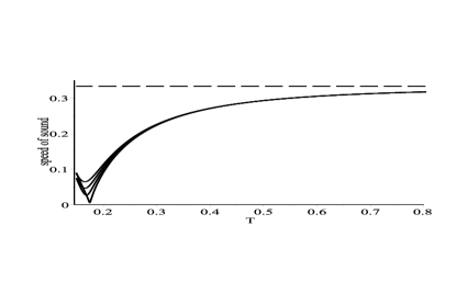
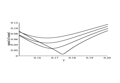
( a )                                                                 ( b )

Figure 1: The squared speed of sound vx .s. temperature at $\mu=0$ for different values of parameter $b$. Curves from top to bottom correspond to $b=-0.0005,-0.0007,-0.0009,-0.0011GeV^{4}$. We enlarge a rectangle region in (a) into (b) to see the detailed structure. For different values of the parameter $b$, the corresponding quasi-transition temperature $T_{0}$, i.e. the position of the minimum value, changes.

III.3 Phase Diagram

For different chemical potentials, the temperature dependence on the horizon $z_{H}$ is showed in FIG. 2. For vanishing or small chemical potential $0\leq\mu\leq\mu_{c}=0.23148GeV$, the temperature decreases monotonously to zero; while for $\mu>\mu_{c}$, the temperature bends up and goes down again to zero. Therefore, for certain range, the same temperature corresponds to three different horizons as indicated in (b) of FIG. 2. This temperature behavior implicates that a phase transition happens at certain temperature for $\mu>\mu_{c}$.

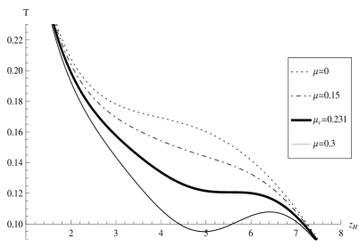
( a )                                                                 ( b )

Figure 2: The temperature v.s. horizon at different chemical potentials $\mu=0,0.15,0.231,0.3GeV$. We enlarge a rectangle region in (a) into (b) to see the detailed structure. For $0<\mu<\mu_{c}$, the temperature decreases monotonously to zero; while for $\mu>\mu_{c}$, the temperature has a local minimum. At $\mu_{c}\simeq 0.231GeV$, the local minimum reduces to a inflection point.

To determine the thermodynamically stability, we plot specific heat $C_{V}$ v.s. temperature $T$ in FIG. 3, where the specific heat $C_{V}$ is defined as

$$C_{V}=T\left(\dfrac{\partial s}{\partial T}\right)_{\mu}.$$ (3.7)

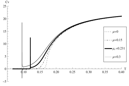
( a )                                                                 ( b )

Figure 3: The specific heat v.s. temperature at different chemical potentials $\mu=0,0.15,0.231,0.3GeV$. We enlarge a rectangle region in (a) into (b) to see the detailed structure. For $0\leq\mu\leq\mu_{c}$, the specific heat is always positive, $C_{V}>0$ implies that the black hole with any temperature is thermodynamically stable. While for $\mu>\mu_{c}$, $C_{V}$ could be negative for a range of $T$ where the black hole is thermodynamically unstable.

In the $C_{V}-T$ diagram, the negative value of the specific heat corresponds to the thermodynamically instability. For $0\leq\mu\leq\mu_{c}$, the specific heat is always positive. $C_{V}>0$ implies that the black hole with any temperature is thermodynamically stable. While for $\mu>\mu_{c}$, $C_{V}$ could be negative for a range of $T$ where the black hole is thermodynamically unstable. Thus one of the three horizons corresponding to the same temperature is thermodynamically unstable and the black hole would never take that state. However, there still left two horizons which are both thermodynamically stable and are possible realistic states. To determined which one is physically preferred out of the two thermodynamically stable states, we need to compare their free energies.

The first law of thermodynamics in a grand canonical ensemble can be written as,

$$F=U-Ts-\mu\rho,$$ (3.8)

where $U$ is the internal energy of the system and $F$ is the corresponding free energy. Changes in the free energy of a system with constant volume are given by

$$dF=-sdT-\rho d\mu.$$ (3.9)

At fixed values of the chemical potential $\mu$, the free energy can be evaluated by the integral 0812.0792 ; 1301.0385

$$F=-\int sdT.$$ (3.10)

Directly integrating shows that the absolute value of the free energy goes to infinity and needs to be regularized. However, since we only care about the differences between the free energies, the absolute values of the free energy are not important for our analysis. Thus we can simply regularize the free energy by fixing the integration constant in the above integral (3.10). Considering the vanishing chemical potential case, we set the free energy at the quasi-transition temperature $T_{0}\approx 170MeV$ to be zero. By requesting $F\left(T_{0}\right)=0$ at $\mu=0$, we finally are able to calculate the free energy as

$$F=\int_{z_{H}}^{z_{H}\left(T_{0}\right)}s\dfrac{dT}{dz_{H}}dz_{H}.$$ (3.11)

The free energy $F$ v.s. temperature $T$ and the phase diagram are plotted in FIG. 4.

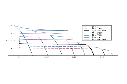
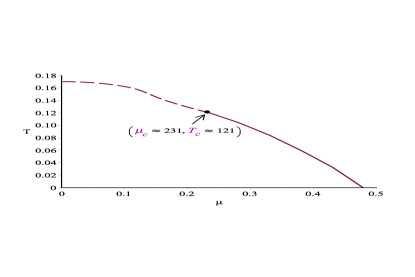
( a )                                                                 ( b )

Figure 4: The free energy v.s. temperature at different chemical potentials $\mu$ is plotted in (a) and the phase diagram in $T$ and $\mu$ plane is plotted in (b). For $0\leq\mu\leq\mu_{c}$, the free energies are single-valued and smooth, the system undergoes a crossover. While for $\mu>\mu_{c}$, the free energies become multi-valued and take swallow-tailed shapes with a first-order phase transition happens at the self-crossing point. At $\mu=\mu_{c}$, the free energy curve is single-valued but not smooth. A second-order phase transition happens at the non-smooth point $\left(\mu_{c},T_{c}\right)\simeq\left(231MeV,121MeV\right)$, which is the critical point where the phase transition mildens to a crossover.

As we expected, for $0\leq\mu\leq\mu_{c}$, the free energies are always single-valued; while for $\mu>\mu_{c}$, the free energies become multi-valued and take swallow-tailed shapes. A first-order phase transition happens at the self-crossing point of each free energy curve with a fixed chemical potential. At $\mu=\mu_{c}$, the free energy curve is continues but not smooth. A second-order phase transition happens at the non-smooth point, which is the critical point where the phase transition mildens to a crossover.

III.4 Equations of State

FIG. 5 plots the squared of speed of sound $c_{s}^{2}$ v.s. the temperature $T$ for different chemical potentials.

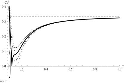
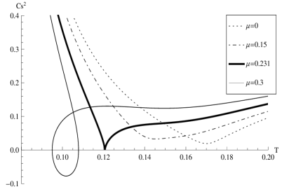
( a )                                                                 ( b )

Figure 5: The squared speed of sound v.s. temperature at different chemical potentials $\mu=0,0.15,0.231,0.3GeV$. We enlarge a rectangle region in (a) into (b) to see the detailed structure. For $0<\mu<\mu_{c}$, the speed of sound behaves as a smooth crossover. At the critical point $\mu=\mu_{c}$, a second order phase transition happens where $c_{s}^{2}$ goes to $0$ at the critical temperature $T_{c}$. For $\mu>\mu_{c}$, the squared of speed of sound undergoes a first order phase transition at the self-crossing point. At high temperature, $c_{s}^{2}$ approaches the conformal limit $1/3$ as expected.

For $0<\mu<\mu_{c}$, the speed of sound behaves as a sharp but smooth crossover. At the critical point $\mu=\mu_{c}$, a second order phase transition happens where $c_{s}^{2}$ goes to $0$ at the critical temperature $T_{c}$. For $\mu>\mu_{c}$, the squared of speed of sound becomes negative, i.e. the speed of sound is imaginary, for a range of temperature. The imaginary speed of sound indicates a Gregory-Laflamme instability 9301052 ; 9404071 . This is related to the general version of Gubser-Mitra conjecture 0009126 ; 0011127 ; 0104071 , i.e. the dynamical stability of a horizon is equivalent to the thermodynamic stability. In our system, the negative specific heat implies thermodynamically unstable. While the imaginary speed of sound implies the amplitude of the fixed momentum sound wave would increase exponentially with time, reflecting the dynamical instability. Roughly speaking, $C_{V}<0$ is equivalent to $c_{s}^{2}<0$ in our system. In all the case, $c_{s}^{2}$ approaches the conformal limit $1/3$ at very high temperature as expected.

We plot equations of state for entropy in FIG. 6. For $0<\mu<\mu_{c}$, the entropy is single-valued and there is no phase transition. For $\mu\geq\mu_{c}$, the entropy is multi-valued for a region of temperature which indicates a phase transition between high entropy and low entropy black holes. The similar phase behaviors have been discussed in 0804.0434 for a holographic QCD model with different values of parameters tuned by hand.

( a )                                                                 ( b )

Figure 6: The entropy v.s. temperature at different chemical potentials $\mu=0,0.15,0.231,0.3GeV$. We enlarge a rectangle region in (a) into (b) to see the detailed structure. For $0<\mu<\mu_{c}$, the entropy is single-valued and there is no phase transition. For $\mu\geq\mu_{c}$, the entropy is multi-valued for a region of temperature which indicates a phase transition between high entropy and low entropy black holes.

The pressure $p=-F$ and the energy $\epsilon=F+sT$ can be calculated from the free energy and are plotted in FIG. 7. We see that both pressure and energy increases with the chemical potential, that pushes the phase transition temperature to the smaller values for growing $\mu$. Our results are consistent to the recent lattice results with finite chemical potential 1204.6710 .

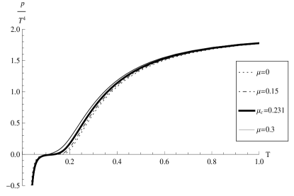
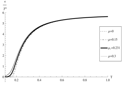
( a )                                                                 ( b )

Figure 7: The equations of state at different chemical potentials $\mu=0,0.15,0.231,0.3GeV$. The pressure v.s. temperature is plotted in (a) and the energy v.s. temperature is plotted in (b).

We finally plot the trace anomaly $\epsilon-3p$ v.s $T$ in FIG. 8. With the growing chemical potential $\mu$, the peak of trace anomaly decreases. From (b) in FIG. 8, we clearly see that, for $0<\mu<\mu_{c}$, the trace anomaly is single-valued with finite slope through all the curve. For $\mu\geq\mu_{c}$, the slope of the trace anomaly becomes infinite at the certain temperature indicating a phase transition happened there.

( a )                                                                 ( b )

Figure 8: The trace anomaly v.s. temperature at different chemical potentials $\mu=0,0.15,0.231,0.3GeV$. We enlarge a rectangle region in (a) into (b) to see the detailed structure. For $0<\mu<\mu_{c}$, the trace anomaly is single-valued with finite slope through all the curve. For $\mu\geq\mu_{c}$, the slope of the trace anomaly becomes infinite at the certain temperature indicating a phase transition happened there.

IV Conclusion

In this paper, we studied a Einstein-Maxwell-dilaton system with a dilaton potential. We consistently solved the equations of motion of the system by the potential reconstruction method. A family of analytic black hole solutions is obtained. We then carefully studied the thermodynamic properties of the black hole backgrounds. We computed the free energy to get the phase diagram of the black hole backgrounds. In its dual holographic QCD theory, we are able to realized the Regge trajectory of the vector mass spectrum by fixing the gauge kinetic function. We then calculated the equations of state in our holographic QCD model. We found that our dynamical model captures many properties in the realistic QCD. The most remarkable feature of our model is that, by changing the chemical potential, we are able to see the conversion from the phase transition to a crossover dynamically. We identified the critical point in our holographic QCD model and calculated its value with $\left(\mu_{c},T_{c}\right)\simeq\left(0.231GeV,0.121GeV\right)$. As the authors knowledge, our model is the first holographic QCD model which could both dynamically describe the transformation from the phase transition to the crossover by changing the chemical potential and realize the linear Regge trajectory for the meson spectrum.

There are many future directions are worth to be studied. For example, one can introduce a open string in the black hole background and compute the linear quark-antiquark potential and expectation value of Polyakov loop to incorporate the confinement-deconfinement phase transition. One can also compute the various transport coefficients like shear viscosity, bulk viscosity and so on. It is also interesting to compute the critical exponents of various physical quantities near the critical point. Some of these issues are in progress.

- (1) O. Philipsen, “Lattice QCD at non-zero temperature and baryon density” [arXiv:1009.4089 [hep-lat]].
- (2) J. Babington, J. Erdmenger, N. J. Evans, Z. Guralnik and I. Kirsch, “Chiral symmetry breaking and pions in nonsupersymmetric gauge / gravity duals,” Phys. Rev. D 69, 066007 (2004) [hep-th/0306018].
- (3) M. Kruczenski, D. Mateos, R. C. Myers and D. J. Winters, “Towards a holographic dual of large N(c) QCD,” JHEP 0405, 041 (2004) [arXiv:hep-th/0311270].
- (4) M. Kruczenski, D. Mateos, R. C. Myers and D. J. Winters, “Meson spectroscopy in AdS / CFT with flavor,” JHEP 0307, 049 (2003) [arXiv:hep-th/0304032].
- (5) S. Kobayashi, D. Mateos, S. Matsuura, R. C. Myers and R. M. Thomson, “Holographic phase transitions at finite baryon density,” JHEP 0702, 016 (2007) [arXiv:hep-th/0611099].
- (6) T. Sakai and S. Sugimoto, “Low energy hadron physics in holographic QCD,” Prog. Theor. Phys. 113, 843 (2005) [arXiv:hep-th/0412141].
- (7) T. Sakai and S. Sugimoto, “More on a holographic dual of QCD,” Prog. Theor. Phys. 114, 1083 (2005) [arXiv:hep-th/0507073].
- (8) J. Erlich, E. Katz, D. T. Son and M. A. Stephanov, “QCD and a holographic model of hadrons,” Phys. Rev. Lett. 95, 261602 (2005) [arXiv:hep-ph/0501128].
- (9) A. Karch, E. Katz, D. T. Son and M. A. Stephanov, “Linear confinement and AdS/QCD,” Phys. Rev. D 74, 015005 (2006) [arXiv:hep-ph/0602229].
- (10) B. Batell and T. Gherghetta, “Dynamical Soft-Wall AdS/QCD,” Phys. Rev. D 78, 026002 (2008) [arXiv:0801.4383 [hep-ph]].
- (11) W. de Paula, T. Frederico, H. Forkel and M. Beyer, “Dynamical AdS/QCD with area-law confinement and linear Regge trajectories,” Phys. Rev. D 79, 075019 (2009) [arXiv:0806.3830 [hep-ph]].
- (12) S. S. Gubser and A. Nellore, “Mimicking the QCD equation of state with a dual black hole,” Phys. Rev. D 78, 086007 (2008) [arXiv:0804.0434 [hep-th]].
- (13) U. Gursoy, E. Kiritsis, L. Mazzanti, G. Michalogiorgakis and F. Nitti, “Improved Holographic QCD,” Lect. Notes Phys. 828, 79 (2011) [arXiv:1006.5461 [hep-th]].
- (14) O. DeWolfe, S. S. Gubser and C. Rosen, “A holographic critical point,” Phys. Rev. D 83, 086005 (2011) [arXiv:1012.1864 [hep-th]].
- (15) O. DeWolfe, S. S. Gubser and C. Rosen, “Dynamic critical phenomena at a holographic critical point,” Phys. Rev. D 84, 126014 (2011) [arXiv:1108.2029 [hep-th]].
- (16) R. -G. Cai, S. He and D. Li, “A hQCD model and its phase diagram in Einstein-Maxwell-Dilaton system,” JHEP 1203, 033 (2012) [arXiv:1201.0820 [hep-th]].
- (17) D. Li, S. He, M. Huang and Q. -S. Yan, “Thermodynamics of deformed AdS5 model with a positive/negative quadratic correction in graviton-dilaton system,” JHEP 1109, 041 (2011) [arXiv:1103.5389 [hep-th]].
- (18) R. -G. Cai, S. Chakrabortty, S. He and L. Li, “Some aspects of QGP phase in a hQCD model,” JHEP 1302 068 (2013) [arXiv:1209.4512 [hep-th]].
- (19) Song He, Shang-Yu Wu, Yi Yang, Pei-Hung Yuan, ”Phase Structure in a Dynamical Soft-Wall Holographic QCD Model”, JHEP 1304 093 (2013) [arXiv:1301.0385 [hep-th]].
- (20) M. Fromm, J. Langelage, S. Lottini and O. Philipsen, “The QCD deconfinement transition for heavy quarks and all baryon chemical potentials,” JHEP 1201, 042 (2012) [arXiv:1111.4953 [hep-lat]].
- (21) Pasi Huovinen and Péter Petreczky, ”QCD Equation of State and Hadron Resonance Gas”, Nucl. Phys. A 837 26-53 (2010) [arXiv:0912.2541 [hep-ph]].
- (22) W. M. Yao et al. (Particle Data Group), J. Phys. G 33, 1 (2006) and 2007 partial update for the 2008 edition.
- (23) Mei Huang, Qi-Shu Yan, Yi Yang, ”Confront Holographic QCD with Regge Trajectories”, Euro. Phys. J. C66, Issue 1 (2010) 187. [arXiv:0710.0988 [hep-ph]].
- (24) Mei Huang, Qi-Shu Yan, Yi Yang, ”Toward a more realistic holographic QCD model”, Prog. Theor. Phys. S 174, 334, (2008) [arXiv:0804.2731 [hep-ph]].
- (25) Jan M. Pawlowski, Fabian Rennecke, ”Higher order quark-mesonic scattering processes and the phase structure of QCD”, [arXiv:1403.1179 [hep-ph]].
- (26) S. Borsanyi et al., ”Is there still any Tc mystery in lattice QCD? Results with physical masses in the continuum limit III”, JHEP 1009 073 (2010), [arXiv:1005.3508 [hep-lat]].
- (27) U. Gursoy, E. Kiritsis, L. Mazzanti and F. Nitti, “Holography and Thermodynamics of 5D Dilaton-gravity,” JHEP 0905, 033 (2009) [arXiv:0812.0792 [hep-th]].
- (28) R. Gregory and R. Laflamme, “Black strings and p-branes are unstable,” Phys. Rev. Lett. 70, 2837 (1993) [arXiv:hep-th/9301052].
- (29) R. Gregory and R. Laflamme, “The Instability of charged black strings and p-branes,” Nucl. Phys. B 428, 399 (1994) [arXiv:hep-th/9404071].
- (30) S. S. Gubser and I. Mitra, “Instability of charged black holes in Anti-de Sitter space” [arXiv:hep-th/0009126].
- (31) S. S. Gubser and I. Mitra, “The Evolution of unstable black holes in anti-de Sitter space,” JHEP 0108, 018 (2001) [arXiv:hep-th/0011127].
- (32) H. S. Reall, “Classical and thermodynamic stability of black branes,” Phys. Rev. D 64, 044005 (2001) [arXiv:hep-th/0104071].
- (33) S. Borsanyi, G. Endrodi, Z. Fodor, S. D. Katz, S. Krieg, C. Ratti and K. K. Szabo, “QCD equation of state at nonzero chemical potential: continuum results with physical quark masses at order ,” JHEP 1208, 053 (2012) [arXiv:1204.6710 [hep-lat]].