A Generic Numbering System based on Catalan Families of Combinatorial Objects

Abstract

We describe arithmetic algorithms on a canonical number representation based on the Catalan family of combinatorial objects specified as a Haskell type class.

Our algorithms work on a generic representation that we illustrate on instances members of the Catalan family, like ordered binary and multiway trees. We validate the correctness of our algorithms by defining an instance of the same type class based the usual bitstring-based natural numbers.

While their average and worst case complexity is within constant factors of their traditional counterparts, our algorithms provide super-exponential gains for numbers corresponding to Catalan objects of low representation size.

Keywords:

tree-based numbering systems, cross-validation with type classes, arithmetic with combinatorial objects, Catalan families, generic functional programming algorithms.

1 Introduction

This paper generalizes the results of [16] and [17], where special instances of the Catalan family [11, 6] of combinatorial objects (the language of balanced parentheses and the set ordered rooted trees with empty leaves, respectively) have been endowed with basic arithmetic operations corresponding to those on bitstring-represented natural numbers and extends [19] with advanced arithmetic operations and computations involving record holding primes and values of the Collatz sequence on gigantic numbers.

The main contribution of this paper is a generic Catalan family based numbering system that supports computations with numbers comparable in size with Knuth’s “arrow-up” notation. These computations have an average and worst case and complexity that is comparable or better than the traditional binary numbers, while on neighborhoods of iterated powers of two they outperform binary numbers by an arbitrary tower of exponents factor.

As the Catalan family contains a large number of computationally isomorphic but structurally distinct combinatorial objects, we will describe our arithmetic computations generically, using Haskell’s type classes [22], of which typical members of the Catalan family, like binary trees and multiway trees will be described as instances.

At the same time, an atypical instance will be derived, representing the set of natural numbers $\mathbb{N}$, which will be used to cross-validate the correctness of our generically defined arithmetic operations.

The paper is organized as follows. Section 2 discusses related work. Section 3 introduces a generic view of Catalan families as a Haskell type class, with subsection 3.4 embedding the set of natural numbers as an instance of the family. Section 4 introduces basic algorithms for arithmetic operations taking advantage of our number representation, with subsection 4.2 focusing on constant time successor and predecessor operations. Section 5 describes arithmetic operations that favor operands of low representation complexity including computations with giant numbers. Section 13 concludes the paper.

We have adopted a literate programming style, i.e. the the code described in the paper forms a self-contained Haskell module (tested with ghc 7.10.2). It is available at http://www.cse.unt.edu/~tarau/research/2014/GCat.hs.

2 Related work

The first instance of a hereditary number system representing natural numbers as multiway trees occurs in the proof of Goodstein’s theorem [2], where replacement of finite numbers on a tree’s branches by the ordinal $\omega$ allows him to prove that a “hailstone sequence”, after visiting arbitrarily large numbers, eventually turns around and terminates.

Another hereditary number system is Knuth’s TCALC program [5] that decomposes $n=2^{a}+b$ with $0\leq b<2^{a}$ and then recurses on $a$ and $b$ with the same decomposition. Given the constraint on $a$ and $b$, while hereditary, the TCALC system is not based on a bijection between $\mathbb{N}$ and $\mathbb{N}\times\mathbb{N}$ and therefore the representation is not a bijection. Moreover, the literate C-program that defines it only implements successor, addition, comparison and multiplication, and does not provide a constant time power of 2 and low complexity leftshift / rightshift operations.

Several notations for very large numbers have been invented in the past. Examples include Knuth’s up-arrow notation [4], covering operations like the tetration (a notation for towers of exponents). In contrast to the tree-based natural numbers we describe in this paper, such notations are not closed under addition and multiplication, and consequently they cannot be used as a replacement for ordinary binary or decimal numbers.

While combinatorial enumeration and combinatorial generation, for which a vast literature exists (see for instance [11], [8] and [6]) can be seen as providing unary Peano arithmetic operations implicitly, like in [16] and [17], the algorithms in this paper enable arithmetic computations of efficiency comparable to the usual binary numbers (or better) using combinatorial families.

Providing a generic mechanism for efficient arithmetic computations with arbitrary members of the Catalan family is the main motivation and the most significant contribution of this paper. It is notationally similar to the type class mechanism sketched in [3]. Unfortunately, the simpler binary tree-based computation of [3] does not support the $O(log^{*}(n))$ successor and predecessor operations described in this paper, that facilitate size proportionate encodings of data types. Such encodings are the critical component of the companion paper [18], which describes their application to lambda terms.

3 The Catalan family of combinatorial objects

The Haskell data type T representing ordered rooted binary trees with empty leaves E and branches provided by the constructor C is a typical member of the Catalan family of combinatorial objects [11].

⬇

data T $=$ E $\mid$ C T T deriving (Eq,Show,Read)

Note the use of the type classes Eq, Show and Read to derive structural equality and respectively human readable output and input for this data type.

The data type M is another well-known member of the Catalan family, defining multiway ordered rooted trees with empty leaves.

⬇

data M $=$ F [M] deriving (Eq,Show,Read)

3.1 A generic view of Catalan families as a Haskell type class

We will work through the paper with a generic data type ranging over instances of the type class Cat, representing a member of the Catalan family of combinatorial objects [11].

⬇

class (Show a,Read a,Eq a) $\Rightarrow$ Cat a where

e :: a

c :: (a,a) $\rightarrow$ a

c’ :: a $\rightarrow$ (a,a)

The zero element is denoted e and we inherit from classes Read and Show which ensure derivation of input and output functions for members of type class Cat as well as from type class Eq that ensures derivation of the structural equality predicate == and its negation /=.

We will also define the corresponding recognizer predicates e_ and c_, relying on the derived equality relation inherited from the Haskell type class Eq.

⬇

e_ :: a $\rightarrow$ Bool

e_ a $=$ a $=$$=$ e

c_ :: a $\rightarrow$ Bool

c_ a $=$ a $/$$=$ e

For each instance, we assume that c and c’ are inverses on their respective domains Cat $\times$ Cat and Cat - {e}, and e is distinct from objects constructed with c, more precisely that the following hold:

$$\forall x.~{}c^{\prime}(c~{}x)=x\land\forall y.~{}(c\_~{}y\Rightarrow c~{}(c^{\prime}~{}y)=y)$$ (1)

$$\forall x.~{}(e\_~{}x\lor c\_~{}x)\land\lnot(e\_~{}x\land c\_~{}x)$$ (2)

When talking about “objects of type Cat” we will actually mean an instance a of the polymorphic type Cat a that verifies equations (1) and (2).

3.2 The instance $\tt T$ of ordered rooted binary trees

The operations defined in type class Cat correspond naturally to the ordered rooted binary tree view of the Catalan family, materialized as the data type $\tt T$.

⬇

instance Cat T where

e $=$ E

c (x,y) $=$ C x y

c’ (C x y) $=$ (x,y)

Note that adding and removing the constructor C trivially verifies the assumption that our generic operations c and c’ are inverses.

3.3 The instance $\tt M$ of ordered rooted multiway trees

The alternative view of the Catalan family as multiway trees is materialized as the data type $\tt M$.

⬇

instance Cat M where

e $=$ F []

c (x,F xs) $=$ F (x:xs)

c’ (F (x:xs)) $=$ (x,F xs)

Note that the assumption that our generic operations c and c’ are inverses is easily verified in this case as well, given the bijection between binary and multiway trees. Moreover, note that operations on types T and M, expressed in terms of their generic type class Cat counterparts, result in a constant extra effort. Therefore, we will safely ignore it when discussing the complexity of different operations.

3.4 An unusual member of the Catalan family: the set of natural numbers $\mathbb{N}$

The (big-endian) binary representation of a natural number can be written as a concatenation of binary digits of the form

$$n=b_{0}^{k_{0}}b_{1}^{k_{1}}\ldots b_{i}^{k_{i}}\ldots b_{m}^{k_{m}}$$ (3)

with $b_{i}\in\{0,1\}$,$~{}b_{i}\neq b_{i+1}$ and the highest digit $b_{m}=1$. The following hold.

Proposition 1

An even number of the form $0^{i}j$ corresponds to the operation $2^{i}j$ and an odd number of the form $1^{i}j$ corresponds to the operation $2^{i}(j+1)-1$.

Proof

It is clearly the case that $0^{i}j$ corresponds to multiplication by a power of $2$. If $f(i)=2i+1$ then it is shown by induction (see [20]) that the $i$-th iterate of $f$, $f^{i}$ is computed as in the equation (4)

$$f^{i}(j)=2^{i}(j+1)-1$$ (4)

Observe that each block $1^{i}$ in $n$, represented as $1^{i}j$ in equation (3), corresponds to the iterated application of $f$, $i$ times, $n=f^{i}(j)$.

Proposition 2

A number $n$ is even if and only if it contains an even number of blocks of the form $b_{i}^{k_{i}}$ in equation (3). A number $n$ is odd if and only if it contains an odd number of blocks of the form $b_{i}^{k_{i}}$ in equation (3).

Proof

It follows from the fact that the highest digit (and therefore the last block in big-endian representation) is $1$ and the parity of the blocks alternate.

This suggests defining the c operation of type class Cat as follows.

$$c(i,j)=\begin{cases}{2^{i+1}j}&{\text{if }j\text{ is odd}},\\ {2^{i+1}(j+1)-1}&{\text{if }j\text{ is even}}.\end{cases}$$ (5)

Note that the exponents are $i+1$ instead of $i$ as we start counting at $0$. Note also that $c(i,j)$ will be even when $j$ is odd and odd when $j$ is even.

Proposition 3

The equation (5) defines a bijection $c:\mathbb{N}\times\mathbb{N}\to\mathbb{N}^{+}=\mathbb{N}-\{0\}$.

Therefore c has an inverse c’, that we will constructively define together with c. The following Haskell code defines the instance of the Catalan family corresponding to $\mathbb{N}$.

⬇

type N $=$ Integer

instance Cat Integer where

e $=$ 0

c (i,j) $\mid$ i$\geq$0 && j$\geq$0 $=$ 2^(i$+$1)$*$(j$+$b)-b where b $=$ mod (j$+$1) 2

The definition of the inverse c’ relies on the dyadic valuation of a number $n$, $\nu_{2}(n)$, defined as the largest exponent of 2 dividing $n$, implemented as the helper function dyadicVal.

⬇

c’ k $\mid$ k$>$0 $=$ (i-1,j-b) where

b $=$ mod k 2

(i,j) $=$ dyadicVal (k$+$b)

dyadicVal k $\mid$ even k $=$ (1$+$i,j) where (i,j) $=$ dyadicVal (div k 2)

dyadicVal k $=$ (0,k)

Note the use of the parity b in both definitions, which differentiates between the computations for even and odd numbers.

The following examples illustrate the use of c and c’ on this instance.

*GCat> c (100,200)
509595541291748219401674688561151
*GCat> c’ it
(100,200)
*GCat> map c’ [1..10]
[(0,0),(0,1),(1,0),(1,1),(0,2),(0,3),(2,0),(2,1),(0,4),(0,5)]
*GCat> map c it
[1,2,3,4,5,6,7,8,9,10]

Figure 1 illustrates the DAG obtained by applying the operation c’ repeatedly and merging identical subtrees for three consecutive numbers. The order of the edges is marked with 0 and 1.

Figure 1: DAG representing the list [2018..2022]

3.5 Other instances using members of the Catalan family of combinatorial objects

The language of balanced parentheses (Dyck words) is another member of the Catalan family, easily seen as in bijection with multiway trees. A convenient representation is one in which a list of positive integers are used to mark the position of each enclosing parenthesis, marked each with a 0. As the offset between opening and closing parenthesis is always even, we adjust that with a linear transformation ensuring the range is the positive integers. Thus ((()())(())) (corresponding to 24) is represented as [3,1,0,1,0,0,2,1,0,0] and (()()()()()()), corresponding to 42 is represented as [1,0,1,0,1,0,1,0,1,0,1,0].

After defining a data type wrapping list of integers, we obtain the instance P of type class Cat.

⬇

data P $=$ P [Int] deriving (Eq,Show,Read)

instance Cat P where

e $=$ P []

c (P xs,P ys) $=$ P ((l:xs)$+$$+$(0:ys)) where l$=$1$+$((length xs) ‘div‘ 2)

c’ (P (l:xs)) $=$ (P (take (x-1) xs),P (drop x xs)) where x $=$ 2$*$l-1

3.6 The transformers: morphing between instances of the Catalan family

As all our instances implement the bijection c and its inverse c’, a generic transformer from an instance to another is defined by the function view:

⬇

view :: (Cat a, Cat b) $\Rightarrow$ a $\rightarrow$ b

view z $\mid$ e_ z $=$ e

view z $\mid$ c_ z $=$ c (view x,view y) where (x,y) $=$ c’ z

To obtain transformers defining bijections with $\mathbb{N},\tt T$ and $\tt M$ as ranges, we will simply provide specialized type declarations for them:

⬇

n :: Cat a $\Rightarrow$ a$\rightarrow$N

n $=$ view

⬇

t :: Cat a $\Rightarrow$ a$\rightarrow$T

t $=$ view

⬇

m :: Cat a $\Rightarrow$ a$\rightarrow$M

m $=$ view

⬇

p :: Cat a $\Rightarrow$ a$\rightarrow$P

p $=$ view

The following examples illustrate the resulting specialized conversion functions:

*GCat> t 42
C E (C E (C E (C E (C E (C E E)))))
*GCat> m it
F [F [],F [],F [],F [],F [],F []]
*GCat> p it
P [1,0,1,0,1,0,1,0,1,0,1,0]
*GCat> n it
42

A list view of an instance of type class Cat is obtained by iterating the constructor c and its inverse c’.

⬇

to_list :: Cat a $\Rightarrow$ a $\rightarrow$ [a]

to_list x $\mid$ e_ x $=$ []

to_list x $\mid$ c_ x $=$ h:hs where

(h,t) $=$ c’ x

hs $=$ to_list t

⬇

from_list :: Cat a $\Rightarrow$ [a] $\rightarrow$ a

from_list [] $=$ e

from_list (x:xs) $=$ c (x,from_list xs)

They work as follows:

*GCat> to_list 2020
[1,0,1,5]
*GCat> from_list it
2020

The function to_list corresponds to the children of a node in the multiway tree view provided by instance M. Along the lines of [13, 14] one can use to_list and from_list to define size-proportionate bijective encodings of sets, multisets and data types built from them.

The function catShow provides a view as a string of balanced parentheses, an instance of the Catalan family for which arithmetic computations are introduced in [16].

⬇

catShow :: Cat a $\Rightarrow$ a $\rightarrow$ [Char]

catShow x $\mid$ e_ x $=$ "()"

catShow x $\mid$ c_ x $=$ r where

xs $=$ to_list x

r $=$ "(" $+$$+$ (concatMap catShow xs) $+$$+$ ")"

It is illustrated below.

*GCat> catShow 0
"()"
*GCat> catShow 1
"(())"
*GCat> catShow 12345
"(()(())(()())(()()())(()))"

4 Generic arithmetic operations on members of the Catalan family

We will now implement arithmetic operations on Catalan families, generically, in terms of the operations on type class Cat.

4.1 Basic utilities

We start with some simple functions to be used later.

4.1.1 Inferring even and odd

As we know for sure that the instance $\mathbb{N}$, corresponding to natural numbers supports arithmetic operations, we will mimic their behavior at the level of the type class Cat.

The operations even_ and odd_ implement the observation following from of Prop. 2 that parity (staring with $1$ at the highest block) alternates with each block of distinct $0$ or $1$ digits.

⬇

even_ :: Cat a $\Rightarrow$ a $\rightarrow$ Bool

even_ x $\mid$ e_ x $=$ True

even_ z $\mid$ c_ z $=$ odd_ y where (_,y)$=$c’ z

odd_ :: Cat a $\Rightarrow$ a $\rightarrow$ Bool

odd_ x $\mid$ e_ x $=$ False

odd_ z $\mid$ c_ z $=$ even_ y where (_,y)$=$c’ z

4.1.2 One

We also provide a constant u and a recognizer predicate u_ for $1$.

⬇

u :: Cat a $\Rightarrow$ a

u $=$ c (e,e)

u_ :: Cat a $\Rightarrow$ a$\rightarrow$ Bool

u_ z $=$ c_ z && e_ x && e_ y where (x,y) $=$ c’ z

4.2 Average constant time successor and predecessor

We will now specify successor and predecessor on the family of data types $\tt Cat$ through two mutually recursive functions, s and s’. They are based on arithmetic observations about the behavior of these blocks when incrementing or decrementing a binary number by 1, derived from equation (5).

They first decompose their arguments using c’. Then, after transforming them as a result of adding or subtracting 1, they place back the results with the c operation.

Note that the two functions work on a block of 0 or 1 digits at a time. The main intuition is that as adding or subtracting 1 changes the parity of a number and as carry-ons propagate over a block of 1s in the case of addition and over a block of 0s in the case of subtraction, blocks of contiguous 0 and 1 digits will be flipped as a result of applying s or s’.

⬇

s :: Cat a $\Rightarrow$ a $\rightarrow$ a

s x $\mid$ e_ x $=$ u -- 1

s z $\mid$ c_ z && e_ y $=$ c (x,u) where -- 2

(x,y) $=$ c’ z

For the general case, the successor function s delegates the transformation of the blocks of $0$ and $1$ digits to functions f and g handling even_ and respectively odd_ cases.

⬇

s a $\mid$ c_ a $=$ if even_ a then f a else g a where

f k $\mid$ c_ w && e_ v $=$ c (s x,y) where -- 3

(v,w) $=$ c’ k

(x,y) $=$ c’ w

f k $=$ c (e, c (s’ x,y)) where -- 4

(x,y) $=$ c’ k

g k $\mid$ c_ w && c_ n && e_ m $=$ c (x, c (s y,z)) where -- 5

(x,w) $=$ c’ k

(m,n) $=$ c’ w

(y,z) $=$ c’ n

g k $\mid$ c_ v $=$ c (x, c (e, c (s’ y, z))) where -- 6

(x,v) $=$ c’ k

(y,z) $=$ c’ v

The predecessor function s’ inverts the work of s as marked by a comment of the form k --, for k ranging from 1 to 6.

⬇

s’ :: Cat a $\Rightarrow$ a $\rightarrow$ a

s’ k $\mid$ u_ k $=$ e where -- 1

(x,y) $=$ c’ k

s’ k $\mid$ c_ k && u_ v $=$ c (x,e) where -- 2

(x,v) $=$ c’ k

For the general case, s’ delegates the transformation of the blocks of $0$ and $1$ digits to functions g and f handling even_ and respectively odd_ cases.

⬇

s’ a $\mid$ c_ a $=$ if even_ a then g’ a else f’ a where

g’ k $\mid$ c_ v && c_ w && e_ r $=$ c (x, c (s y,z)) where -- 6

(x,v) $=$ c’ k

(r,w) $=$ c’ v

(y,z) $=$ c’ w

g’ k $\mid$ c_ v $=$ c (x,c (e, c (s’ y, z))) where -- 5

(x,v) $=$ c’ k

(y,z) $=$ c’ v

f’ k $\mid$ c_ v && e_ r $=$ c (s x,z) where -- 4

(r,v) $=$ c’ k

(x,z) $=$ c’ v

f’ k $=$ c (e, c (s’ x,y)) where -- 3

(x,y) $=$ c’ k

One can see that their use matches successor and predecessor on instance N:

*GCat> map s [0..15]
[1,2,3,4,5,6,7,8,9,10,11,12,13,14,15,16]
*GCat> map s’ it
[0,1,2,3,4,5,6,7,8,9,10,11,12,13,14,15]

Proposition 4

Denote $\tt Cat^{+}=\tt Cat-\{\text{\tt e}\}$. The functions $s:\tt Cat\to\tt Cat^{+}$ and $s^{\prime}:\tt Cat^{+}\to\tt Cat$ are inverses.

Proof

For each instance of $\tt Cat$, it follows by structural induction after observing that patterns for rules marked with the number -- k in s correspond one by one to patterns marked by -- k in s’ and vice versa.

More generally, it can be shown that Peano’s axioms hold and as a result $<\tt Cat,e,s>$ is a Peano algebra. This is expected, as s provides a combinatorial enumeration of the infinite stream of Catalan objects, as illustrated below on instance T:

Cats> s E
C E E
*GCat> s it
C E (C E E)
*GCat> s it
C (C E E) E

The function nums generates an initial segment of the “natural numbers” defined by an instance of Cat.

⬇

nums :: Cat a $\Rightarrow$ a $\rightarrow$ [a]

nums x $=$ f x [] where

f x xs $\mid$ e_ x $=$ e:xs

f x xs $=$ f (s’ x) (x:xs)

Note that if parity information is kept explicitly, the calls to odd_ and even_ are constant time, as we will assume in the rest of the paper. We will also assume, that when complexity is discussed, a representation like the tree data types $\tt T$ or $\tt M$ are used, making the operations c and c’ constant time. Note also that this is clearly not the case for the instance N using the traditional bitstring representation where effort proportional to the length of the bitstring may be involved.

Proposition 5

The worst case time complexity of the s and s’ operations on an input $n$ is given by the iterated logarithm $O(log_{2}^{*}(n))$.

Proof

Note that calls to s,s’ in s or s’ happen on terms at most logarithmic in the bitsize of their operands. The recurrence relation counting the worst case number of calls to s or s’ is: $T(n)=T({{log_{2}(n)}})+O(1)$, which solves to $T(n)=O(log_{2}^{*}(n))$.

Note that this is much better than the logarithmic worst case for binary numbers (when computing, for instance, binary 111…111+1=1000…000).

Proposition 6

s and s’ are constant time, on the average.

Proof

When computing the successor or predecessor of a number of bitsize $n$, calls to s,s’ in s or s’ happen on at most one subterm. Observe that the average size of a contiguous block of 0s or 1s in a number of bitsize $n$ has the upper bound 2 as ${\sum_{k=0}^{n}{1\over 2^{k}}}=2-{1\over{2^{n}}}<2$. As on 2-bit numbers we have an average of $0.25$ more calls, we can conclude that the total average number of calls is constant, with upper bound $2+0.25=2.25$.

A quick empirical evaluation confirms this. When computing the successor on the first $2^{30}=1073741824$ natural numbers, there are in total 2381889348 calls to s and s’, averaging to 2.2183 per computation. The same average for $100$ successor computations on $5000$ bit random numbers oscillates around $2.22$.

4.3 A few other average constant time, $O(log^{*})$ worst case operations

We will derive a few operations that inherit their complexity from s and s’.

4.3.1 Double and half

Doubling a number db and reversing the db operation (hf) are quite simple. For instance, db proceeds by adding a new counter for odd numbers and incrementing the first counter for even ones.

⬇

db :: Cat a $\Rightarrow$ a $\rightarrow$ a

db x $\mid$ e_ x $=$ e

db x $\mid$ odd_ x $=$ c (e,x)

db z $=$ c (s x,y) where (x,y) $=$ c’ z

⬇

hf :: Cat a $\Rightarrow$ a $\rightarrow$ a

hf x $\mid$ e_ x $=$ e

hf z $\mid$ e_ x $=$ y where (x,y) $=$ c’ z

hf z $=$ c (s’ x,y) where (x,y) $=$ c’ z

4.3.2 Power of 2 and its left inverse

Note that such efficient implementations follow directly from simple number theoretic observations.

For instance, exp2, computing an power of $2$ , has the following definition in terms of c and s’ from which it inherits its complexity up to a constant factor.

⬇

exp2 :: Cat a $\Rightarrow$ a $\rightarrow$ a

exp2 x $\mid$ e_ x $=$ u

exp2 x $=$ c (s’ x, u)

The same applies to its left inverse log2:

⬇

log2 :: Cat a $\Rightarrow$ a $\rightarrow$ a

log2 x $\mid$ u_ x $=$ e

log2 x $\mid$ u_ z $=$ s y where (y,z) $=$ c’ x

Proposition 7

The operations db, hf, exp2 and log2 are average constant time and are ${log}^{*}$ in the worst case.

Proof

At most one call to s,s’ is made in each definition. Therefore these operations have the same worst and average complexity as s and s’.

We illustrate their work on instances N:

*GCat> map exp2 [0..14]
[1,2,4,8,16,32,64,128,256,512,1024,2048,4096,8192,16384]
*GCat> map log2 it
[0,1,2,3,4,5,6,7,8,9,10,11,12,13,14]

More interestingly, a tall tower of exponents that would overflow memory on instance N, is easily supported on instances T and M as shown below:

*GCat> exp2 (exp2 (exp2 (exp2 (exp2 (exp2 (exp2 E))))))
C (C (C (C (C (C E E) E) E) E) E) (C E E)
*GCat> m it
F [F [F [F [F [F [F []]]]]],F []]
*GCat> log2 (log2 (log2 (log2 (log2 (log2 (log2 it))))))
F []

This example illustrates the main motivation for defining arithmetic computation with the “typical” members of the Catalan family: their ability to deal with giant numbers.

Another average constant time / worst case $log^{*}$ algorithm is counting the trailing 0s of a number (on instance $\tt T$):

⬇

trailingZeros x $\mid$ e_ x $=$ e

trailingZeros x $\mid$ odd_ x $=$ e

trailingZeros x $=$ s (fst (c’ x))

This contrasts with the O(log(n) worst case performance to count them with a bitstring representation.

5 Addition, subtraction and their mutually recursive helpers

We will derive in this section efficient addition and subtraction that work on one run-length compressed block at a time, rather than by individual 0 and 1 digit steps.

5.1 Multiplication by a power of 2

We start with the functions leftshiftBy, leftshiftBy’ and leftshiftBy” corresponding respectively to $(\lambda x.2x)^{n}(k)$ , $(\lambda x.2x+1)^{n}(k)$ and $(\lambda x.2x+2)^{n}(k)$.

The function leftshiftBy prefixes an odd number with a block of $1$s and extends a block of $0$s by incrementing their count.

⬇

leftshiftBy :: Cat a $\Rightarrow$ a $\rightarrow$ a $\rightarrow$ a

leftshiftBy x y $\mid$ e_ x $=$ y

leftshiftBy _ y $\mid$ e_ y $=$ e

leftshiftBy x y $\mid$ odd_ y $=$ c (s’ x, y)

leftshiftBy x v $=$ c (add x y, z) where (y,z) $=$ c’ v

The function leftshiftBy’ is based on equation (6).

$$(\lambda x.2x+1)^{n}(k)=2^{n}(k+1)-1$$ (6)

⬇

leftshiftBy’ :: Cat a $\Rightarrow$ a $\rightarrow$ a $\rightarrow$ a

leftshiftBy’ x k $=$ s’ (leftshiftBy x (s k))

The function leftshiftBy’ is based on equation (7) (see [20] for a direct proof by induction).

$$(\lambda x.2x+2)^{n}(k)=2^{n}(k+2)-2$$ (7)

⬇

leftshiftBy’’ :: Cat a $\Rightarrow$ a $\rightarrow$ a $\rightarrow$ a

leftshiftBy’’ x k $=$ s’ (s’ (leftshiftBy x (s (s k))))

They are part of a chain of mutually recursive functions as they are already referring to the add function. Note also that instead of naively iterating, they implement a more efficient algorithm, working “one block at a time”. For instance, when detecting that its argument counts a number of 1s, leftshiftBy’ just increments that count. As a result, the algorithm favors numbers with relatively few large blocks of 0 and 1 digits.

While not directly used in the addition operation it is interesting to observe that division by a power of 2 can also be computed efficiently.

5.2 An inverse operation: division by a power of 2

The function rightshiftBy goes over its argument y one block at a time, by comparing the size of the block and its argument x that is decremented after each block by the size of the block. The local function f handles the details, irrespectively of the nature of the block, and stops when the argument is exhausted. More precisely, based on the result EQ, LT, GT of the comparison, f either stops or, calls rightshiftBy on the the value of x reduced by the size of the block a’ = s a.

⬇

rightshiftBy :: Cat a $\Rightarrow$ a $\rightarrow$ a $\rightarrow$ a

rightshiftBy x y $\mid$ e_ x $=$ y

rightshiftBy _ y $\mid$ e_ y $=$ e

rightshiftBy x y $=$ f (cmp x a’) where

(a,b) $=$ c’ y

a’ $=$ s a

f LT $=$ c (sub a x,b)

f EQ $=$ b

f GT $=$ rightshiftBy (sub x a’) b

5.3 Addition optimized for numbers built from a few large blocks of 0s and 1s

We are now ready to define addition. The base cases are

⬇

add :: Cat a $\Rightarrow$ a $\rightarrow$ a $\rightarrow$ a

add x y $\mid$ e_ x $=$ y

add x y $\mid$ e_ y $=$ x

In the case when both terms represent even numbers, the two blocks add up to an even block of the same size. Note the use of cmp and sub in helper function f to trim off the larger block such that we can operate on two blocks of equal size.

⬇

add x y $\mid$even_ x && even_ y $=$ f (cmp a b) where

(a,as) $=$ c’ x

(b,bs) $=$ c’ y

f EQ $=$ leftshiftBy (s a) (add as bs)

f GT $=$ leftshiftBy (s b) (add (leftshiftBy (sub a b) as) bs)

f LT $=$ leftshiftBy (s a) (add as (leftshiftBy (sub b a) bs))

In the case when the first term is even and the second odd, the two blocks add up to an odd block of the same size.

⬇

add x y $\mid$even_ x && odd_ y $=$ f (cmp a b) where

(a,as) $=$ c’ x

(b,bs) $=$ c’ y

f EQ $=$ leftshiftBy’ (s a) (add as bs)

f GT $=$ leftshiftBy’ (s b) (add (leftshiftBy (sub a b) as) bs)

f LT $=$ leftshiftBy’ (s a) (add as (leftshiftBy’ (sub b a) bs))

In the case when the second term is even and the first odd the two blocks also add up to an odd block of the same size.

⬇

add x y $\mid$odd_ x && even_ y $=$ add y x

In the case when both terms represent odd numbers, we use the identity (8):

$${(\lambda x.2x+1)}^{k}(x)+{(\lambda x.2x+1)}^{k}(y)={(\lambda x.2x+2)}^{k}(x+y)$$ (8)

⬇

add x y $\mid$ odd_ x && odd_ y $=$ f (cmp a b) where

(a,as) $=$ c’ x

(b,bs) $=$ c’ y

f EQ $=$ leftshiftBy’’ (s a) (add as bs)

f GT $=$ leftshiftBy’’ (s b) (add (leftshiftBy’ (sub a b) as) bs)

f LT $=$ leftshiftBy’’ (s a) (add as (leftshiftBy’ (sub b a) bs))

Note the presence of the comparison operation cmp also part of our chain of mutually recursive operations. Note also the local function f that in each case ensures that a block of the same size is extracted, depending on which of the two operands a or b is larger.

Details of implementation for subtraction are quite similar to those of the addition. The curious reader can find the implementation and the literate programming explanations of the complete set of arithmetic operations with the type class Cat in our arxiv draft at [15].

Comparison

The comparison operation cmp provides a total order (isomorphic to that on $\mathbb{N}$) on our generic type $\tt Cat$. It relies on bitsize computing the number of binary digits constructing a term in $\tt Cat$, also part of our mutually recursive functions, to be defined later.

We first observe that only terms of the same bitsize need detailed comparison, otherwise the relation between their bitsizes is enough, recursively. More precisely, the following holds:

Proposition 8

Let bitsize count the number of digits of a base-2 number, with the convention that it is 0 for 0. Then bitsize$(x)<$bitsize$(y)\Rightarrow x<y$.

Proof

Observe that their lexicographic enumeration ensures that the bitsize of base-2 numbers is a non-decreasing function.

The comparison operation also proceeds one block at a time, and it also takes some inferential shortcuts, when possible.

⬇

cmp :: Cat a$\Rightarrow$ a$\rightarrow$a$\rightarrow$Ordering

cmp x y $\mid$ e_ x && e_ y $=$ EQ

cmp x _ $\mid$ e_ x $=$ LT

cmp _ y $\mid$ e_ y $=$ GT

cmp x y $\mid$ u_ x && u_ (s’ y) $=$ LT

cmp x y $\mid$ u_ y && u_ (s’ x) $=$ GT

For instance, it is easy to see that comparison of x and y can be reduced to comparison of bitsizes when they are distinct. Note that bitsize, to be defined later, is part of the chain of our mutually recursive functions.

⬇

cmp x y $\mid$ x’ $/$$=$ y’ $=$ cmp x’ y’ where

x’ $=$ bitsize x

y’ $=$ bitsize y

When bitsizes are equal, a more elaborate comparison needs to be done, delegated to function compBigFirst.

⬇

cmp xs ys $=$ compBigFirst True True (rev xs) (rev ys) where

rev $=$ from_list . reverse . to_list

The function compBigFirst compares two terms known to have the same bitsize. It works on reversed (highest order digit first) variants, computed by reverse and it takes advantage of the block structure using the following proposition:

Proposition 9

Assuming two terms of the same bitsizes, the one with $1$ as its first before the highest order digit, is larger than the one with $0$ as its first before the highest order digit.

Proof

Observe that little-endian numbers obtained by applying the function rev are lexicographically ordered with $0<1$.

As a consequence, cmp only recurses when identical blocks lead the sequence of blocks, otherwise it infers the LT or GT relation.

⬇

compBigFirst _ _ x y $\mid$ e_ x && e_ y $=$ EQ

compBigFirst False False x y $=$ f (cmp a b) where

(a,as) $=$ c’ x

(b,bs) $=$ c’ y

f EQ $=$ compBigFirst True True as bs

f LT $=$ GT

f GT $=$ LT

compBigFirst True True x y $=$ f (cmp a b) where

(a,as) $=$ c’ x

(b,bs) $=$ c’ y

f EQ $=$ compBigFirst False False as bs

f LT $=$ LT

f GT $=$ GT

compBigFirst False True x y $=$ LT

compBigFirst True False x y $=$ GT

The following examples illustrate the agreement of cmp with the usual order relation on $\mathbb{N}$.

*GCat> cmp 5 10
LT
*GCat> cmp 10 10
EQ
*GCat> cmp 10 5
GT

Note that the complexity of the comparison operation is proportional to the size of the (smaller) of the two trees.

The function bitsize, last in our chain of mutually recursive functions, computes the number of digits, except that we define it as e for constant function e (corresponding to 0). It works by summing up the counts of 0 and 1 digit blocks composing a tree-represented natural number.

⬇

bitsize :: Cat a $\Rightarrow$ a $\rightarrow$ a

bitsize z $\mid$ e_ z $=$ z

bitsize z $=$ s (add x (bitsize y)) where (x,y) $=$ c’ z

It follows that the base-2 integer logarithm is computed as

⬇

ilog2 :: Cat a $\Rightarrow$ a$\rightarrow$a

ilog2 $=$ s’ . bitsize

5.3.1 Subtraction

The code for the subtraction function sub is similar to that for addition:

⬇

sub :: Cat a $\Rightarrow$ a $\rightarrow$ a $\rightarrow$ a

sub x y $\mid$ e_ y $=$ x

sub x y $\mid$ even_ x && even_ y $=$ f (cmp a b) where

(a,as) $=$ c’ x

(b,bs) $=$ c’ y

f EQ $=$ leftshiftBy (s a) (sub as bs)

f GT $=$ leftshiftBy (s b) (sub (leftshiftBy (sub a b) as) bs)

f LT $=$ leftshiftBy (s a) (sub as (leftshiftBy (sub b a) bs))

The case when both terms represent 1 blocks the result is a 0 block:

⬇

sub x y $\mid$ odd_ x && odd_ y $=$ f (cmp a b) where

(a,as) $=$ c’ x

(b,bs) $=$ c’ y

f EQ $=$ leftshiftBy (s a) (sub as bs)

f GT $=$ leftshiftBy (s b) (sub (leftshiftBy’ (sub a b) as) bs)

f LT $=$ leftshiftBy (s a) (sub as (leftshiftBy’ (sub b a) bs))

The case when the first block is 1 and the second is a 0 block is a 1 block:

⬇

sub x y $\mid$ odd_ x && even_ y $=$ f (cmp a b) where

(a,as) $=$ c’ x

(b,bs) $=$ c’ y

f EQ $=$ leftshiftBy’ (s a) (sub as bs)

f GT $=$ leftshiftBy’ (s b) (sub (leftshiftBy’ (sub a b) as) bs)

f LT $=$ leftshiftBy’ (s a) (sub as (leftshiftBy (sub b a) bs))

Finally, when the first block is 0 and the second is 1 an identity dual to (8) is used:

⬇

sub x y $\mid$ even_ x && odd_ y $=$ f (cmp a b) where

(a,as) $=$ c’ x

(b,bs) $=$ c’ y

f EQ $=$ s (leftshiftBy (s a) (sub1 as bs))

f GT $=$ s (leftshiftBy (s b) (sub1 (leftshiftBy (sub a b) as) bs))

f LT $=$ s (leftshiftBy (s a) (sub1 as (leftshiftBy’ (sub b a) bs)))

sub1 x y $=$ s’ (sub x y)

Note that these algorithms collapse to the ordinary binary addition and subtraction most of the time, given that the average size of a block of contiguous 0s or 1s is 2 bits (as shown in Prop. 6), so their average complexity is within constant factor of their ordinary counterparts.

On the other hand, as they are limited by the representation size of the operands rather than their bitsize, when compared with their bitstring counterparts, these algorithms favor deeper trees made of large blocks, representing giant “towers of exponents”-like numbers by working (recursively) one block at a time rather than 1 bit at a time, resulting in possibly super-exponential gains on them.

The following examples illustrate the agreement with their usual counterparts:

*GCat> map (add 10) [0..15]
[10,11,12,13,14,15,16,17,18,19,20,21,22,23,24,25]
*GCat> map (sub 15) [0..15]
[15,14,13,12,11,10,9,8,7,6,5,4,3,2,1,0]

6 Algorithms for advanced arithmetic operations

6.1 Multiplication, optimized for large blocks of 0s and 1s

Devising a similar optimization as for add and sub for multiplication (mul) is actually easier.

After making sure that the recursion is on its smaller argument, mul delegates its work to mul1 which uses the decomposition of the first argument based on equation (5). When the first term represents an even number, mul1 applies the leftshiftBy operation corresponding to $2^{x+1}zy$, otherwise it derives a similar operation from the representation $(2^{x+1}(z+1)-1)y$.

⬇

mul :: Cat a $\Rightarrow$ a $\rightarrow$ a $\rightarrow$ a

mul x y $=$ f (cmp x y) where

f GT $=$ mul1 y x

f _ $=$ mul1 x y

mul1 :: Cat a $\Rightarrow$ a $\rightarrow$ a $\rightarrow$ a

mul1 x _ $\mid$ e_ x $=$ e

mul1 x y $\mid$ u_ x $=$ y

mul1 a y $\mid$ even_ a $=$

leftshiftBy (s x) (mul1 z y) where (x,z) $=$ c’ a

mul1 a y $\mid$ odd_ a $=$

sub (leftshiftBy (s x) (mul1 (s z) y)) y where (x,z) $=$ c’ a

Note that when the operands are composed of large blocks of alternating 0 and 1 digits, the algorithm is quite efficient as it works (roughly) in time depending on the the number of blocks in its first argument rather than its number of digits. The following example illustrates a blend of arithmetic operations benefiting from complexity reductions on giant tree-represented numbers:

*GCat> let term1 =
    sub (exp2 (exp2 (t 12345))) (exp2 (t 6789))
*GCat> let term2 =
    add (exp2 (exp2 (t 123))) (exp2 (t 456789))
*GCat> bitsize (bitsize (mul term1 term2))
C E (C E (C E (C (C E (C E E))
   (C (C E (C E (C E E))) (C (C E E) E)))))
*GCat> n it
12346

6.2 Power

After specializing our multiplication for a squaring operation,

⬇

square x $=$ mul x x

we can implement a simple but efficient “power by squaring” operation for $x^{y}$, as follows:

⬇

pow _ x $\mid$ e_ x $=$ c (x,x)

pow a b $\mid$ even_ a $=$ c (s’ (mul (s x) b),ys) where

(x,xs) $=$ c’ a

ys $=$ pow xs b

pow a b $\mid$ even_ b $=$ pow (superSquare y a) ys where

(y,ys) $=$ c’ b

superSquare a x $\mid$ e_ a $=$ square x

superSquare k x $=$ square (superSquare (s’ k) x)

pow x y $=$ mul x (pow x (s’ y))

It works well with fairly large numbers, by also benefiting from efficiency of multiplication on terms with large blocks of 0 and 1 digits:

*GCat> n (bitsize (pow (t 10) (t 100)))
333
*GCat> pow (t 32) (t 10000000)
C (C (C E (C (C E E) E)) (C (C (C E E) (C E E)) (C (C (C E E) E)
  (C E (C E (C E (C (C (C E E) (C E E)) (C E (C E E))))))))) (C E E)

6.3 General division

An algorithm derived from the well known long division is given here. While it matches its bitstring equivalent asymptotically, it does not provide the same complexity gains as, for instance, multiplication, addition or subtraction.

⬇

div_and_rem :: Cat a $\Rightarrow$ a $\rightarrow$ a $\rightarrow$ (a, a)

div_and_rem x y $\mid$ LT $=$$=$ cmp x y $=$ (e,x)

div_and_rem x y $\mid$ c_ y $=$ (q,r) where

(qt,rm) $=$ divstep x y

(z,r) $=$ div_and_rem rm y

q $=$ add (exp2 qt) z

The function divstep implements a step of the division operation.

⬇

divstep n m $=$ (q, sub n p) where

q $=$ try_to_double n m e

p $=$ leftshiftBy q m

The function try_to_double doubles its second argument while smaller than its first argument and returns the number of steps it took. This value will be used by divstep when applying the leftshiftBy operation.

⬇

try_to_double x y k $=$

if (LT$=$$=$cmp x y) then s’ k

else try_to_double x (db y) (s k)

By specializing div_and_rem we derive division and remainder.

⬇

divide :: Cat b $\Rightarrow$ b $\rightarrow$ b $\rightarrow$ b

divide n m $=$ fst (div_and_rem n m)

remainder :: Cat b $\Rightarrow$ b $\rightarrow$ b $\rightarrow$ b

remainder n m $=$ snd (div_and_rem n m)

The following examples illustrate the agreement with their usual counterparts:

*GCat> divide 26 3
8
*GCat> remainder 26 3
2

7 Specialized Arithmetic Operations and Primality Tests

We describe in this section a number of special purpose arithmetic operations showing the practical usefulness of our number representation.

7.1 Integer Square Root

A fairly efficient integer square root, using Newton’s method, is implemented as follows:

⬇

isqrt x $\mid$ e_ x $=$ x

isqrt n $=$ if cmp (square k) n$=$$=$GT then s’ k else k where

two $=$ c (e,(c (e,e)))

k$=$iter n

iter x $=$ if cmp (absdif r x) two $=$$=$ LT

then r

else iter r where r $=$ step x

step x $=$ divide (add x (divide n x)) two

absdif x y $=$ if LT $=$$=$ cmp x y then sub y x else sub x y

The following examples illustrate the agreement with their usual counterparts:

*GCat> isqrt (t 101)
C E (C E (C E (C E E)))
*GCat> n it
10

7.2 Modular Power

The modular power operation $x^{y}(mod~{}m)$ can be optimized to avoid the creation of large intermediate results, by combining “power by squaring” and pushing the modulo operation inside the inner function modStep.

⬇

modPow m base expo $=$ modStep expo one base where

one $=$ c (e,e)

modStep x r b $\mid$ x $=$$=$ one $=$ (mul r b) ‘remainder‘ m

modStep x r b $\mid$ odd_ x $=$

modStep (hf (s’ x)) (remainder (mul r b) m)

(remainder (square b) m)

modStep x r b $=$ modStep (hf x) r (remainder (square b) m)

The following examples illustrate the correctness of these operations:

*GCat> modPow (t 10) (t 3) (t 3)
C (C E (C E E)) E
*GCat> n it
7

7.3 Lucas-Lehmer Primality Test for Mersenne Numbers

The Lucas-Lehmer primality test has been used for the discovery of all the record holder largest known prime numbers of the form $2^{p}-1$ with $p$ prime in the last few years. It is based on iterating $p-2$ times the function $f(x)=x^{2}-2$, starting from $x=4$. Then $2^{p}-1$ is prime if and only if the result modulo $2^{p}-1$ is $0$, as proven in [1]. The function ll_iter implements this iteration.

⬇

ll_iter k n m $\mid$e_ k $=$ n

ll_iter k n m $=$ fastmod y m where

x $=$ ll_iter (s’ k) n m

y $=$ s’ (s’ (square x))

It relies on the function fastmod which provides a specialized fast computation of $k~{}modulo~{}(2^{p}-1)$.

⬇

fastmod k m $\mid$ k $=$$=$ s’ m $=$ e

fastmod k m $\mid$ LT $=$$=$ cmp k m $=$ k

fastmod k m $=$ fastmod (add q r) m where

(q,r) $=$ div_and_rem k m

Finally the Lucas-Lehmer primality test is implemented as follows:

⬇

lucas_lehmer p $\mid$ p $=$$=$ s (s e) $=$ True

lucas_lehmer p $=$ e $=$$=$ (ll_iter p_2 four m) where

p_2 $=$ s’ (s’ p)

four $=$ c (c (e,e),c (e,e))

m $=$ exp2 p

We illustrate its use for detecting a few Mersenne primes:

*GCat> map n (filter lucas_lehmer (map t [3,5..31]))
[3,5,7,13,17,19,31]
*GCat> map (\p->2^p-1) it
[7,31,127,8191,131071,524287,2147483647]

Note that the last line contains the Mersenne primes corresponding to $2p+1$.

7.4 Miller-Rabin Probabilistic Primality Test

Let $\nu_{2}(x)$ denote the dyadic valuation of x, i.e., the largest exponent of 2 that divides x. The function dyadicSplit defined by equation (9)

$$dyadicSplit(k)={(k,{k\over 2^{\nu_{2}(k)}})}$$ (9)

can be implemented as an average constant time operation as:

⬇

dyadicSplit z $\mid$ odd_ z $=$ (e,z)

dyadicSplit z $\mid$ even_ z $=$ (s x, s xs) where

(x,xs) $=$ c’ (s’ z)

After defining a sequence of k random natural numbers in an interval

⬇

randomNats :: (Cat a) $\Rightarrow$ Int $\rightarrow$ Int $\rightarrow$ a $\rightarrow$ a $\rightarrow$ [a]

randomNats seed k smallest largest $=$ map view ns where

ns $=$ take k (randomRs

(n smallest,n largest) (mkStdGen seed))

we are ready to implement the function oddPrime that runs k tests and concludes primality with probability $1-{1\over 4^{k}}$ if all k calls to function strongLiar succeed.

⬇

oddPrime :: Cat a $\Rightarrow$ Int $\rightarrow$ a $\rightarrow$ Bool

oddPrime k m $=$ all strongLiar as where

one $=$ s e

two $=$ s one

m’ $=$ s’ m

as $=$ randomNats k k two m’

(l,d) $=$ dyadicSplit m’

strongLiar a $=$ (x $=$$=$ one $\mid$$\mid$ (any ($=$$=$ m’) (squaringSteps l x))) where

x $=$ modPow m a d

squaringSteps x _ $\mid$ e_ x $=$ []

squaringSteps l x $=$ x:squaringSteps (s’ l)

(remainder (square x) m)

Note that we use dyadicSplit to find a pair (l,d) such that l is the largest power of t 2 dividing the predecessor m’ of the suspected prime m. The function strongLiar checks, for a random base a, a condition that primes (but possibly also a few composite numbers) verify.

Finally isProbablyPrime handles the case of even numbers and calls oddPrime with the parameter specifying the number of tests, k=42.

⬇

isProbablyPrime x $\mid$ x$=$$=$two $=$ True where two $=$ s (s e)

isProbablyPrime x $\mid$ even_ x $=$ False

isProbablyPrime p $=$ oddPrime 42 p

The following example illustrates the correct behavior of the algorithm on a the interval [2..100].

*GCat> map n (filter isProbablyPrime (map t [2..100]))
[2,3,5,7,11,13,17,19,23,29,31,37,41,43,47,53,59,61,67,71,73,79,83,89,97]

8 Boolean Operations on Tree-represented Bitvectors

We implement bitvector operations (also seen as efficient bitset operations) to work “one block of binary digits at a time”, to facilitate their use on large but sparse boolean formulas involving a large numbers of variables. One will be able to evaluate such formulas “all value-combinations at a time” when represented as bitvectors of size $2^{2^{n}}$. Note that such operations will be tractable with our trees, provided that they have a relatively small representation complexity, despite their large bitsize.

8.1 Bitwise Operations One Block of Digits at a time

We implement a generic bitwise operation that takes a boolean function bf as its first parameter.

First, when an argument is F [], corresponding to 0 the behavior is derived from that of the boolean function bf.

⬇

bitwise :: (Cat a) $\Rightarrow$ (Bool $\rightarrow$ Bool $\rightarrow$ Bool) $\rightarrow$ a $\rightarrow$ a $\rightarrow$ a

bitwise bf x y $\mid$ e_ x && e_ y $=$ x

bitwise bf x y $\mid$ e_ x $=$ if bf False True then y else x

bitwise bf x y $\mid$ e_ y $=$ if bf True False then x else y

Next, the parities of the arguments px and py are used to derive the parity of the result pz, by applying the boolean function bz.

⬇

bitwise bf x y $=$ f (cmp a b) where

(a,as) $=$ c’ x

(b,bs) $=$ c’ y

px $=$ odd_ x

py $=$ odd_ y

pz $=$ bf px py

Based on the parity pz the local function f (also parameterized by the result of the comparison between arguments x and y) is called.

⬇

f EQ $=$ fApply bf pz (s a) as bs

f GT $=$ fApply bf pz (s b) (fromB px (sub a b) as) bs

f LT $=$ fApply bf pz (s a) as (fromB py (sub b a) bs)

The function f calls fromB to derive from the parities px and py the appropriate left-shifting operation.

⬇

fromB False $=$ leftshiftBy

fromB True $=$ leftshiftBy’

Finally, the function f calls the helper function fApply, which, depending on the expected parity of the result pz, applies the appropriate left-shift operation to the result of the recursive application of bitwise to the remaining blocks of digits u and tt v.

⬇

fApply bf False k u v $=$ leftshiftBy k (bitwise bf u v)

fApply bf True k u v $=$ leftshiftBy’ k (bitwise bf u v)

The actual bitwise operations are obtained by parameterizing the generic bitwise function with the appropriate Haskell boolean functions:

⬇

bitwiseOr x y$=$ bitwise ($\mid$$\mid$) x y

bitwiseXor x y $=$ bitwise ($/$$=$) x y

bitwiseAnd x y $=$ bitwise (&&) x y

Bitwise negation (requiring the additional parameter k to specify the intended bitlength of the operand) corresponds to the complement w.r.t. the “universal set” of all natural numbers up to $2^{k}-1$. It is defined as usual, by subtracting from the “bitmask” corresponding to $2^{k}-1$:

⬇

bitwiseNot k x $=$ sub y x where y $=$ s’ (exp2 k)

The function bitwiseAndNot combines bitwiseOr, bitwiseNot the usual way, except that it uses the helper function bitsOf to ensure enough mask bits are made available when negation is applied.

⬇

bitwiseAndNot x y $=$ bitwiseNot l d where

l $=$ max2 (bitsOf x) (bitsOf y)

d $=$ bitwiseOr (bitwiseNot l x) y

The function bitsOf adapts our definition for bitsize to compute the number of bits of a bitvector (considering 0 to be 1 bit).

⬇

bitsOf x $\mid$ e_ x $=$ s x

bitsOf x $=$ bitsize x

The following example illustrates that our bitwise operations can be efficiently applied to giant numbers:

*GCat> bitwiseXor (s (exp2 (exp2 (m 12345))))  (s’ (exp2 (exp2 (m 6789))))
F [F [],F [F [],F [F [F []],F [F [F []],F []],F [],F [],F [],F [],
  F [F []]]],F [F [F [F []],F [],F [F [F []]],F [],F [],F [],F [],
  F [F []]],F [],F [F [],F [],F [F []],F [F []],F [],F [F []],F [],
  F [],F [],F []]],F []]

Note that while the size of the term representing this result is 46 F nodes the bitsize of the result is $2^{12346}$ showing clearly that such an operation is intractable with a bitstring representation.

8.2 Boolean Formula Evaluation

Besides definitions for the bitwise boolean functions, we also need definitions of the projection variables $var(n,k)$ corresponding to column $k$ of a truth table, for a function with $n$ variables. A compact formula for them, as given in [7] or [21], is

$$var(n,k)=({{2^{2^{n}}-1})~{}/~{}({2^{2^{n-k-1}}+1}})$$ (10)

However, instead of doing the division, one can compute them as a concatenation of alternating blocks of $1$ and $0$ bits to take advantage of our efficient block operations.

⬇

var n k $=$ repeatBlocks nbBlocks blockSize mask where

k’ $=$ s k

nbBlocks $=$ exp2 k’

blockSize $=$ exp2 (sub n k’)

mask $=$ s’ (exp2 blockSize)

The alternating blocks are put together by the function repeatBlocks that shifts to the left by the size of a block, at each step, and adds the mask made of $2^{n-k}$ ones, at each even step.

⬇

repeatBlocks x _ _ $\mid$ e_ x $=$ x

repeatBlocks k l mask $=$

if odd_ k then r else add mask r where

r $=$ leftshiftBy l (repeatBlocks (s’ k) l mask)

The following examples illustrate these operations:

*GCat> map n (map (var (t 3)) (map t [0..2]))
[15,51,85]
*GCat> map n (map (var (t 4)) (map t [0..3]))
[255,3855,13107,21845]
*GCat> map n (map (var (t 5)) (map t [0..4]))
[65535,16711935,252645135,858993459,1431655765]

The following example illustrates the evaluation of a boolean formula in conjunctive normal form (CNF). The mechanism is usable as a simple satisfiability or tautology tester, for formulas resulting in possibly large but sparse or dense, low structural complexity bitvectors.

⬇

cnf tf $=$ andN (map orN cls) where

cls $=$ [[v0’,v1’,v2],[v0,v1’,v2],

[v0’,v1,v2’],[v0’,v1’,v2’],[v0,v1,v2]]

v0 $=$ var (tf 3) (tf 0)

v1 $=$ var (tf 3) (tf 1)

v2 $=$ var (tf 3) (tf 2)

v0’ $=$ bitwiseNot (exp2 (tf 3)) v0

v1’ $=$ bitwiseNot (exp2 (tf 3)) v1

v2’ $=$ bitwiseNot (exp2 (tf 3)) v2

orN (x:xs) $=$ foldr bitwiseOr x xs

andN (x:xs) $=$ foldr bitwiseAnd x xs

The execution of the function cnf evaluates the formula, the result corresponding to bitvector 88 = [0,0,0,1,1,0,1,0].

*GCat> cnf t
C (C E (C E E)) (C (C E E) (C E (C E E)))
*GCat> cnf m
F [F [F [],F []],F [F []],F [],F []]
*GCat> cnf n
88

9 Representing Sets

9.1 The Bijection between sequences and sets

Increasing sequences provide a canonical representation for sets of natural numbers. While finite sets and finite lists of elements of $\mathbb{N}$ share a common representation [N], sets are subject to the implicit constraint that their ordering is immaterial. This suggest that a set like $[4,1,9,3]$ could be represented canonically as a sequence by first ordering it as $[1,3,4,9]$ and then computing the differences between consecutive elements i.e. $[x_{0},x_{1}\ldots x_{i},x_{i+1}\ldots]\rightarrow[x_{0},x_{1}-x_{0},\ldots x_{i+1}-x_{i}\ldots]$. This gives $[1,2,1,5]$, with the first element $1$ followed by the increments $[2,1,5]$

Therefore, incremental sums, computed with Haskell’s scanl, are used to transform arbitrary lists to canonically represented sets of natural numbers, inverted by pairwise differences computed using zipWith.

⬇

list2set [] $=$ []

list2set (n:ns) $=$ scanl add n ns

set2list [] $=$ []

set2list (m:ms) $=$ m : zipWith sub ms (m:ms)

9.2 The bijections between natural numbers and sets of natural numbers

By composing with natural number-to-list bijections, we obtain bijections to sets of natural numbers.

⬇

to_set x $=$ list2set (to_list x)

from_set x $=$ from_list (set2list x)

As the following example shows, trees offer a significantly more compact representation of sparse sets than conventional binary numbers.

*GCat> n (bitsize (from_set (map t [42,1234,6789])))
6792
*GCat> n (catsize (from_set (map t [42,1234,6789])))
33

Note that a similar compression occurs for sets of natural numbers with only a few elements missing (that we call dense sets), as they have the same representation size as their sparse complement.

*GCat> n (catsize (from_set (map t ([1,3,5]++[6..220]))))
438
*GCat> n (bitsize (from_set (map t ([1,3,5]++[6..220]))))
438

The following holds:

Proposition 10

These encodings/decodings of lists and sets as trees are size-proportionate i.e., their representation sizes are within constant factors.

10 Representation complexity

While a precise average complexity analysis of our algorithms is beyond the scope of this paper, arguments similar to those about the average behavior of s and s’ can be carried out to prove that for all our operations, their average complexity matches their traditional counterparts, using the fact, shown in the proof of Prop. 6, that the average size of a block of contiguous 0 or 1 bits is at most 2.

10.1 Complexity as representation size

To evaluate the best and worst case space requirements of our number representation, we introduce here a measure of representation complexity, defined by the function catsize that counts the non-empty nodes of an object of type $\tt Cat$.

⬇

catsize :: Cat a $\Rightarrow$ a $\rightarrow$ a

catsize z $\mid$ e_ z $=$ z

catsize z $=$ s (add (catsize x) (catsize y)) where (x,y) $=$ c’ z

The following holds:

Proposition 11

For all terms $t\in\tt Cat$, catsize t $\leq$ bitsize t.

Proof

By induction on the structure of $t$, observing that the two functions have similar definitions and corresponding calls to catsize return terms inductively assumed smaller than those of bitsize.

The following example illustrates their use:

*GCat> map catsize [0,100,1000,10000]
[0,7,9,13]
*GCat> map catsize [2^16,2^32,2^64,2^256]
[5,6,6,6]
*GCat> map bitsize [2^16,2^32,2^64,2^256]
[17,33,65,257]

Figure 2 shows the reductions in representation complexity compared with bitsize for an initial interval of $\mathbb{N}$, from $0$ to $2^{10}-1$.

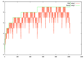
Figure 2: Representation complexity (lower line) bounded by bitsize (upper line)

10.2 Enumerating objects of given representation size

The total number of Catalan objects corresponding to $n$ is given by:

$$C_{n}={1\over{n+1}}{{2n}\choose n}$$ (11)

It is shown in [11] that if $L_{n}={{2^{2n}}\over{n^{3\over 2}}\sqrt{\pi}}$ then ${\lim_{n\to\infty}{C_{n}\over L_{n}}}=1$ , providing an asymptotic bound for $C_{n}$.

The function cat describes an efficient computation for of the Catalan number $C_{n}$ using a direct recursion formula derived from equation (11).

⬇

cat :: N$\rightarrow$N

cat 0 $=$ 1

cat n $\mid$ n$>$0 $=$ (2$*$(2$*$n-1)$*$(cat (n-1))) ‘div‘ (n$+$1)

The first few members of the sequence are computed below:

*GCat> map cat [0..14]
[1,1,2,5,14,42,132,429,1430,4862,16796,58786,208012,742900,2674440]

The following holds.

Proposition 12

Let k = catsize x where x is an object of type $\tt Cat$. Then x relates to k as follows, for instances of $\tt Cat$:

1. x is a binary tree of type $\tt T$ with $k$ internal nodes and $k+1$ leaves

2. x is a multiway tree of type $\tt M$ with $k+1$ nodes

3. x is a term of the type $\tt P$ with $2k+2$ matching parentheses.

Proof

Observe that catsize k counts the $C_{\tt k}-1$ number of C constructors in objects of size k of type T. The rest is a consequence of well-known relations between Catalan numbers and nodes of binary trees, nodes of multiway trees and parentheses in Dyck words as given in [11].

The function catsized enumerates for each of our instances, the objects of size k corresponding to a given Catalan number.

⬇

catsized :: Cat a $\Rightarrow$ a $\rightarrow$ [a]

catsized a $=$ take k [x $\mid$ x$\leftarrow$iterate s e,catsize x $=$$=$ a] where

k $=$ fromIntegral (cat (n a))

The function extracts exactly k elements (with k the Catalan number corresponding to size a) from the infinite enumeration of Catalan objects of type Cat provided by iterate s e, as illustrated below:

*GCat> catsized (t 2)
[C E (C E E),C (C E E) E]
*GCat> catsized 4
[8,9,10,11,12,13,14,16,30,31,63,127,255,65535]

10.3 Best and worst cases

Next we define the higher order function iterated that applies k times the function f, which, contrary to Haskell’s iterate, returns only the final element rather than building the infinite list of all iterates.

⬇

iterated :: Cat a $\Rightarrow$ (t $\rightarrow$ t) $\rightarrow$ a $\rightarrow$ t $\rightarrow$ t

iterated f k x $\mid$e_ k $=$ x

iterated f k x $=$ f (iterated f (s’ k) x)

We can exhibit, for a given bitsize, a best case

⬇

bestCase :: Cat a $\Rightarrow$ a $\rightarrow$ a

bestCase k $=$ iterated f k e where f x $=$ c (x,e)

and a worst case

⬇

worstCase :: Cat a $\Rightarrow$ a $\rightarrow$ a

worstCase k $=$ iterated f k e where f x $=$ c (e,x)

The following examples illustrate these functions:

*GCat> bestCase (t 5)
C (C (C (C (C E E) E) E) E) E
*GCat> n (bitsize (bestCase (t 5)))
65536
*GCat> n (catsize (bestCase (t 5)))
5
*GCat> worstCase (t 5)
C E (C E (C E (C E (C E E))))
*GCat> n (bitsize (worstCase (t 5)))
5
*GCat> n (catsize (worstCase (t 5)))
5

The function bestCase computes the iterated exponent of 2 (tetration) and then applies the predecessor to it. For $k=4$ it corresponds to

${(2^{{{(2^{{{(2^{{{(2^{{0+1}}-1)}+1}}-1)}+1}}-1)}+1}}-1)}=2^{2^{2^{2}}}-1=65535$.

For $k=5$ it corresponds to $2^{65536}-1$.

Note that our concept of representation complexity is only a weak approximation of Kolmogorov complexity [10]. For instance, the reader might notice that our worst case example is computable by a program of relatively small size. However, as bitsize is an upper limit to catsize, we can be sure that we are within constant factors from the corresponding bitstring computations, even on random data of high Kolmogorov complexity.

Note also that an alternative concept of representation complexity can be defined by considering the (vertices+edges) size of the DAG obtained by folding together identical subtrees.

10.4 A Concept of duality

As our instances of Cat are members of the Catalan family of combinatorial objects, they can be seen as binary trees with empty leaves. Therefore, we can transform the tree representation of our objects by swapping left and right branches under a binary tree view, recursively. The corresponding Haskell code is:

⬇

dual :: Cat a $\Rightarrow$ a $\rightarrow$ a

dual x $\mid$ e_ x $=$ e

dual z $=$ c (dual y,dual x) where (x,y) $=$ c’ z

As clearly dual is an involution (i.e., dual $\circ$ dual is the identity of $\tt Cat$), the corresponding permutation of $\mathbb{N}$ will bring together huge and small natural numbers sharing representations of the same size, as illustrated by the following example.

*GCat> map dual [0..20]
[0,1,3,2,4,15,7,6,12,31,65535,16,8,255,127,5,11,8191,4294967295,32,65536]
*CatsBM> catShow 10
"(()()()())"
*CatsBM> catShow (dual 10)
"((((()))))"

For instance, 18 and its dual 4294967295 have representations of the same size, except that the wide tree associated to 18 maps to the tall tree associated to 4294967295, as illustrated by Fig. 3, with trees folded to DAGs by merging together shared subtrees. Note the significantly different bitsizes that can result for a term and its dual.

(a) 18

(b) dual of 18

Figure 3: 18 and its dual, with multiway trees folded to DAGs

*GCat> m 18
F [F [],F [],F [F []],F []]
*GCat> dual (m 18)
F [F [F [F [F []],F []]]]
*GCat> n (bitsize (m 18))
5
*GCat> n (bitsize (dual (m 18)))
32

It follows immediately from the definitions of the respective functions, that, as an extreme case, the following holds:

Proposition 13

$\forall$x. dual (bestCase x) = worstCase x.

The following example illustrates it, with a tower of exponents 10000 tall, reached by bestCase. Note that we run it on objects of type T, as it would dramatically overflow memory on bitstring-represented numbers of type $\mathbb{N}$.

*GCat> dual (bestCase (t 10000)) == worstCase (t 10000)
True

Another interesting property of dual is illustrated by the following examples:

*GCat> [x|x<-[0..2^5-1],cmp (t x) (dual (t x)) ==  LT]
[2,5,6,8,9,10,11,13,14,17,18,19,20,21,22,23,25,26,27,28,29,30]
*GCat> [x|x<-[0..2^5-1],cmp (t x) (dual (t x)) ==  EQ]
[0,1,4,24]
*GCat> [x|x<-[0..2^5-1],cmp (t x) (dual (t x)) ==  GT]
[3,7,12,15,16,31]

The discrepancy between the number of elements for which x is smaller than (dual x) and those for which it is greater or equal, is growing as numbers get larger, contrary to the intuition that, as dual is an involution, the grater and smaller sets would have similar sizes for an initial interval of $\mathbb{N}$. For instance, between $0$ and $2^{16}-1$ one will find only $68$ numbers for which the dual is smaller and $11$ for which it is equal.

Note that random elements of $\mathbb{N}$ tend to have relatively shallow (and wide) multiway tree representations, given that the average size of a contiguous block of 0s or 1s is 2. Consequently, dual provides an interesting bijection between “incompressible” natural numbers (of high Kolmogorov complexity) and their deep, highly compressible, duals.

The existence of such a bijection (computed by a program of constant size) between natural numbers of high and low Kolmogorov complexity reveals a somewhat non-intuitive aspect of this concept and its use for the definition of randomness [10].

We will explore next definitions for concepts of depth for our number representation.

10.5 Representation Depth

As we can switch between the binary and multiway view of our Catalan objects, we will define two sets of representation-depth functions. They use the the helper functions minimum min2 and maximum max2.

⬇

min2, max2 :: Cat a $\Rightarrow$ a $\rightarrow$ a $\rightarrow$ a

min2 x y $=$ if LT$=$$=$cmp x y then x else y

max2 x y $=$ if LT$=$$=$cmp x y then y else x

Corresponding to the binary tree view exemplified by instance T, we define maxTdepth returning the length of the longest path from the root to a leaf.

⬇

maxTdepth :: Cat a $\Rightarrow$ a $\rightarrow$ a

maxTdepth z $\mid$ e_ z $=$ z

maxTdepth z $=$ s (max2 (maxTdepth x) (maxTdepth y)) where (x,y) $=$ c’ z

Corresponding to the multiway tree view exemplified by instance M we define maxTdepth returning the length of the longest path from the root to a leaf.

⬇

maxMdepth :: Cat a $\Rightarrow$ a $\rightarrow$ a

maxMdepth z $\mid$ e_ z $=$ z

maxMdepth z $=$ s (foldr max2 m ms) where

(m:ms) $=$ map maxMdepth (to_list z)

The following simple facts hold, derived from properties of binary and multiway rooted ordered trees.

Proposition 14

Let ${\tt x}\geq{\tt y}$ stand for cmp x y == GT and $=$ stand for cmp x y == EQ.

1. For all objects x of type $\tt Cat$, catsize x $\geq$ maxTdepth x $\geq$ maxMdepth x.

2. For all objects x of type $\tt Cat$, catsize x = catsize (dual x)

3. For all objects x of type $\tt Cat$ maxTdepth x = maxTdepth (dual x).

4. For all objects x of type $\tt Cat$, maxMdepth (bestCase x) $=$ x.

11 Compact representation and tractable computations with some giant numbers

We will illustrate the representation and computation power of our new numbering system with two case studies. The first shows that several record holder primes have compact Catalan representations.

The second shows computation of the hailstone sequence for an equivalent of the Collatz conjecture on giant numbers.

11.1 Record holder primes

Interestingly, most record holder giant primes have a fairly simple structure: they are of the form $p=i2^{k}\pm j$ with $i\in\mathbb{N}$ and $j\in\mathbb{N}$ comparatively small. This is a perfect fit for our representation which favors numbers “in the neighborhood” of linear combinations of (towers of) exponents of two with comparatively small coefficients, resulting in large contiguous blocks of $0$s and $1$s when represented as bitstrings.

The largest known primes (as of early 2019) of several types are given by the following Haskell code.

⬇

mersennePrime f $=$ s’ (exp2 (f 82589933))

generizedFermatPrime f $=$ s (leftshiftBy (f 9167433) (f 27653))

cullenPrime f $=$ s (leftshiftBy x x) where x $=$ f 6679881

woodallPrime f $=$ s’ (leftshiftBy x x) where x $=$ f 3752948

prothPrime f $=$ s (leftshiftBy (f 13018586) (f 19249))

sophieGermainPrime f $=$ s’ (leftshiftBy (f 666667) (f 18543637900515))

twinPrimes f $=$ (s’ y,s y) where

y $=$ leftshiftBy (f 666669) (f 3756801695685)

For instance, the largest known prime, having about 17 million decimal digits, (a Mersenne number) has an unusually small Catalan representation as illustrated below:

*GCat> catShow (mersennePrime t)
"(((())(())()(()())(()())(()())((()))(())()(()())(())()))"
*GCat> n (catsize (mersennePrime t))
27
*GCat> n (bitsize (mersennePrime t))
82589933

Note the use of parameter t indicating that computation proceeds with type T, as it would overflow memory with with bitstring-represented natural numbers.

Figure 4 summarizes comparative bitstring and Catalan representation sizes bitsize and catsize for record holder primes.

Record holder prime	bitsize	catsize
Mersenne prime	82,589,933	27
Generalized Fermat prime	9,167,448	37
Cullen prime	6,679,904	46
Woodall prime	3,752,970	37
Sophie Germain prime	666,712	62
Twin primes 1	666,711	59
Twin primes 2	666,711	60

Figure 4: Bitsizes vs. Catalan representation sizes of record holder primes

*GCat> catShow (genFermatPrime t)
"(()((()())(()())()(())()(()())((())())()()(()())())
  ()()()(()(()))(())()(()))"
*GCat> catShow (cullenPrime t)
"(()((()())(()())()()()()(())()((()))()()(())(()))()
 (())()(())()()()()(())()((()))()()(())(()))"
*GCat> catShow (woodallPrime t)
"((()()()()(()()())((()))()()()(())(()()))(())(()()())
 ((()))()()()(())(()()))"
*GCat> catShow (sophieGermainPrime t)
"((()()()()()()((()))(())()()(()())()()())()()(()())(()())(())
 (())()()(())(())(())((()))()(())((()))(())()(()())()(())((()))())"
*GCat> catShow (fst (twinPrimes t))
"(((())(())()()((()))(())()()(()())()()())(())()(()())(()(()))(())
 ()(())()()()()(())()()(())(())()()()()()()()(())()(()))"
*GCat> catShow (snd (twinPrimes t))
"(()((())()()()()((()))(())()()(()())()()())()()()(()())(()(()))(())
 ()(())()()()()(())()()(())(())()()()()()()()(())()(()))"
*GCat> catShow (snd (mersenne48 t))

*GCat> catsize (dual (sophieGermainPrime t))
C E (C (C (C E E) (C E E)) E)
*GCat> n it
62
*GCat> catsize (dual (prothPrime t))
C E (C (C E E) (C E (C E (C E E))))
*GCat> n it
41
*GCat> catsize (add (dual (prothPrime t)) (dual (sophieGermainPrime t)))
C (C E E) (C E (C E (C E (C (C E E) (C (C E E) E)))))
*GCat> n it
404

11.2 Computing the Collatz/Syracuse sequence for huge numbers

As an interesting application, that achieves something one cannot do with traditional arbitrary bitsize integers is to explore the behavior of interesting conjectures in the “new world” of numbers limited not by their sizes but by their representation complexity. The Collatz conjecture [9] states that the function

$$collatz(x)=\begin{cases}x\over 2&\text{if $x$ is even},\\ 3x+1&\text{if $x$ is odd}.\\ \end{cases}$$ (12)

reaches $1$ after a finite number of iterations. An equivalent formulation, by grouping together all the division by 2 steps, is the function:

$$collatz^{\prime}(x)=\begin{cases}x\over 2^{\nu_{2}(x)}&\text{if $x$ is even},\\ 3x+1&\text{if $x$ is odd}.\\ \end{cases}$$ (13)

where $\nu_{2}(x)$ denotes the dyadic valuation of x, i.e., the largest exponent of 2 that divides x. One step further, the syracuse function is defined as the odd integer $k^{\prime}$ such that $n=3k+1=2^{\nu_{2}(n)}k^{\prime}$. One more step further, by writing $k^{\prime}=2m+1$ we get a function that associates $k\in\mathbb{N}$ to $m\in\mathbb{N}$.

The function tl computes efficiently the equivalent of

$$tl(k)={{{k\over 2^{\nu_{2}(k)}}-1}\over 2}$$ (14)

Together with its hd counterpart, it is defined as

⬇

hd x $=$ fst (decons x)

tl x $=$ snd (decons x)

decons a $\mid$ even_ a $=$ (s x,hf (s’ xs)) where (x,xs) $=$ c’ a

decons a $=$ (e,hf (s’ a))

where the function decons is the inverse of

⬇

cons (x,y) $=$ leftshiftBy x (s (db y))

corresponding to $2^{x}~{}(2y+1)$. Then our variant of the syracuse function corresponds to

$$syracuse(n)=tl(3n+2)$$ (15)

which is defined from $\mathbb{N}$ to $\mathbb{N}$ and can be implemented as

⬇

syracuse :: Cat b $\Rightarrow$ b $\rightarrow$ b

syracuse n $=$ tl (add n (db (s n)))

Note that all operations except the addition add are constant average time.

The function nsyr computes the iterates of this function, until (possibly) stopping:

⬇

nsyr :: Cat t $\Rightarrow$ t $\rightarrow$ [t]

nsyr x $\mid$ e_ x $=$ [e]

nsyr x $=$ x : nsyr (syracuse x)

It is easy to see that the Collatz conjecture is true if and only if nsyr terminates for all $n$, as illustrated by the following example:

*GCat> nsyr 2019
[2019,3029,4544,3408,2556,1917,2876,2157,3236,2427,3641,5462,2048,1536,1152,
 864,648,486,182,68,51,77,116,87,131,197,296,222,83,125,188,141,212,159,239,
 359,539,809,1214,455,683,1025,1538,288,216,162,30,11,17,26,2,0]

Moreover, in this formulation, the conjecture implies that the the elements of sequence generated by nsyr are all different.

The next examples will show that computations for nsyr can be efficiently carried out for giant numbers that, with the traditional bitstring representation, would easily overflow the memory of a computer with more transistors than the atoms in the known universe.

And finally something we are quite sure has never been computed before, we can also start with a tower of exponents 100 levels tall:

*GCat> take 100 (map(n . catsize) (nsyr (bestCase (t 100))))
[100,199,297,298,300,...,440,436,429,434,445,439]

Note that we have only computed the decimal equivalents of the representation complexity catsize of these numbers, which, obviously, would not fit themselves in a decimal representation.

A slightly longer computation (taking a few minutes) can be also performed on a twin tower of exponents 101 and 103 levels tall like in

*GCat> take 2 (map(n.catsize) (nsyr
         (add (bestCase (t 101)) (bestCase (t 103)))))
[10206,10500]

where the Catalan representation size at 10500, proportional to the product of the representation sizes of the operands, slows down computation but still keeps it in a tractable range.

12 Discussion

Our Catalan families based numbering system provides compact representations of giant numbers and can perform interesting computations intractable with their bitstring-based counterparts.

This ability comes from the fact that our canonical tree representation, in contrast to the traditional binary representation supports constant average time and space application of exponentials.

We have not performed a precise time and space complexity analysis (except for the the constant average-time operations), but our experiments indicate that (low) polynomial bounds are likely for addition and subtraction with worst cases of size expansion happening with towers of exponents, where results are likely to be proportional to the product of the height of the towers, as illustrated in subsection 11.2.

Our multiplication and division algorithms are derived from relatively simple traditional ones, with some focus on taking advantage of large blocks of $0$ and $1$ digits. However, it would be interesting to further explore asymptotically better algorithms like Karatsuba multiplication or division based on Newton’s method.

As most numbers have high Kolmogorov complexity, it makes sense to extend our type class mechanism to devise a hybrid numbering system that switches between representations as needed, to delegate cases where there are no benefits, to the underlying bitstring representation. This is likely to be needed for designing a practical extension with Catalan representations for the arithmetic subsystem used in a programming language like Haskell that benefits from the very fast C-based GMP library.

13 Conclusion

We have described through a type class mechanism an arithmetic system working on members of the Catalan family of combinatorial objects, that takes advantage of compact representations of some giant numbers and can perform interesting computations intractable with their bitstring-based counterparts.

This ability comes from the fact that tree representation, in contrast to the traditional binary representation, supports constant average time and space application of exponentials.

The resulting numbering system is canonical - each natural number is represented as a unique object. Besides unique decoding, canonical representations allow testing for syntactic equality. It is also generic – no commitment is made to a particular member of the Catalan family – our type class provides all the arithmetic operations to several instances, including typical members of the Catalan family together with the usual natural numbers.

While these algorithms share similar complexity with those described in [17], which focuses on instance M of our type class Cat, the generic implementation in this paper enables one to perform efficient arithmetic operations with any of the 58 known instances of the Catalan family described in [12, 11], some of them with geometric, combinatorial, algebraic, formal languages, number and set theoretical or physical flavor. Therefore, we believe that this generalization is significant and it opens the door to new and possibly unexpected applications.

Appendix

A subset of Haskell as an executable function notation

We mention, for the benefit of the reader unfamiliar with Haskell, that a notation like f x y stands for $f(x,y)$, [t] represents sequences of type t and a type declaration like f :: s -> t -> u stands for a function $f:s\times t\to u$ (modulo Haskell’s “currying” operation, given the isomorphism between the function spaces ${s\times t}\to u$ and ${s\to t}\to u$).

Our Haskell functions are always represented as sequences of recursive equations guided by pattern matching, conditional to constraints (boolean relations following the “|” symbol and before the “=” symbol) in an equation.

Locally scoped helper functions are defined in Haskell after the “where” keyword, using the same equational style. The composition of functions f and g is denoted f . g. It is customary in Haskell to write $f=g$ instead of $f~{}x=g~{}x$ (“point-free” notation). We make some use of Haskell’s “call-by-need” evaluation that allows us to work with infinite sequences, like the [0..] infinite list notation, as well as higher order functions (having other functions as arguments). Note also that the result of the last evaluation is stored in the special Haskell variable it.

By restricting ourselves to this “Haskell - -” subset, our code can also be easily transliterated into a system of rewriting rules, other pattern-based functional languages as well as deterministic Horn Clauses.

References

- [1] Bruce, J.W.: A Really Trivial Proof of the Lucas-Lehmer Test. The American Mathematical Monthly 100(4), 370–371 (1993)
- [2] Goodstein, R.: On the restricted ordinal theorem. Journal of Symbolic Logic (9), 33–41 (1944)
- [3] Haraburda, D., Tarau, P.: Binary trees as a computational framework. Computer Languages, Systems & Structures 39(4), 163 – 181 (2013)
- [4] Knuth, D.E.: Mathematics and Computer Science: Coping with Finiteness. Science 194(4271), 1235 –1242 (1976)
- [5] Knuth, D.E.: TCALC (1994), http://www-cs-faculty.stanford.edu/~uno/programs/tcalc.w.gz
- [6] Knuth, D.E.: The Art of Computer Programming, Volume 4, Fascicle 4: Generating All Trees–History of Combinatorial Generation (Art of Computer Programming). Addison-Wesley Professional (2006)
- [7] Knuth, D.E.: The Art of Computer Programming, Volume 4, Fascicle 1: Bitwise Tricks & Techniques; Binary Decision Diagrams. Addison-Wesley Professional (2009)
- [8] Kreher, D.L., Stinson, D.: Combinatorial Algorithms: Generation, Enumeration, and Search. The CRC Press Series on Discrete Mathematics and its Applications, CRC PressINC (1999)
- [9] Lagarias, J.C.: The 3x+1 Problem: An Annotated Bibliography (1963–-1999) (2008), http://arXiv.org, 0309224v11
- [10] Li, M., Vitányi, P.: An introduction to Kolmogorov complexity and its applications. Springer-Verlag New York, Inc., New York, NY, USA (1993)
- [11] Stanley, R.P.: Enumerative Combinatorics. Wadsworth Publ. Co., Belmont, CA, USA (1986)
- [12] Stanley, R.P.: Catalan Addendum (2013), http://www-math.mit.edu/~rstan/ec/catadd.pdf
- [13] Tarau, P.: A Groupoid of Isomorphic Data Transformations. In: Carette, J., Dixon, L., Coen, C.S., Watt, S.M. (eds.) Intelligent Computer Mathematics, 16th Symposium, Calculemus, 8th International Conference MKM . pp. 170–185. Springer, LNAI 5625, Grand Bend, Canada (Jul 2009)
- [14] Tarau, P.: Bijective Collection Encodings and Boolean Operations with Hereditarily Binary Natural Numbers. In: PPDP ’14: Proceedings of the 16th international ACM SIGPLAN Symposium on Principles and Practice of Declarative Programming. ACM, New York, NY, USA (2014)
- [15] Tarau, P.: A Generic Numbering System based on Catalan Families of Combinatorial Objects. CoRR abs/1406.1796 (2014)
- [16] Tarau, P.: Computing with Catalan Families. In: Dediu, A.H., Martin-Vide, C., Sierra, J.L., Truthe, B. (eds.) Proceedings of Language and Automata Theory and Applications, 8th International Conference, LATA 2014. pp. 564–576. Springer, LNCS, Madrid, Spain, (Mar 2014)
- [17] Tarau, P.: The Arithmetic of Recursively Run-length Compressed Natural Numbers. In: Ciobanu, G., Méry, D. (eds.) Proceedings of 8th International Colloquium on Theoretical Aspects of Computing, ICTAC 2014. pp. 406–423. Springer, LNCS 8687, Bucharest, Romania (Sep 2014)
- [18] Tarau, P.: A Size-proportionate Bijective Encoding of Lambda Terms as Catalan Objects endowed with Arithmetic Operations. In: Gavanelli, M., Reppy, J. (eds.) Proceedings of the Eighteenth International Symposium on Practical Aspects of Declarative Languages PADL’16. pp. 99–116. Springer, LNCS, St. Petersburg, Florida, USA (Jan 2016)
- [19] Tarau, P.: Computing with Catalan Families, Generically. In: Gavanelli, M., Reppy, J. (eds.) Proceedings of the Eighteenth International Symposium on Practical Aspects of Declarative Languages PADL’16. pp. 117–134. Springer, LNCS, St. Petersburg, Florida, USA (Jan 2016)
- [20] Tarau, P., Buckles, B.: Arithmetic Algorithms for Hereditarily Binary Natural Numbers. In: Proceedings of SAC’14, ACM Symposium on Applied Computing, PL track. pp. 1593–1600. ACM, Gyeongju, Korea (Mar 2014)
- [21] Tarau, P., Luderman, B.: Boolean Evaluation with a Pairing and Unpairing Function. In: Voronkov, A., Negru, V., Ida, T., Jebelean, T., Petcu, D., Watt, S., Zaharie, D. (eds.) Proceedings of SYNASC 2012. pp. 384–392. IEEE (Jan 2013)
- [22] Wadler, P., Blott, S.: How to make ad-hoc polymorphism less ad-hoc. In: POPL. pp. 60–76 (1989)