Non-Poissonian Quantum Jumps of a Fluxonium Qubit due to Quasiparticle Excitations

Abstract

As the energy relaxation time of superconducting qubits steadily improves, non-equilibrium quasiparticle excitations above the superconducting gap emerge as an increasingly relevant limit for qubit coherence. We measure fluctuations in the number of quasiparticle excitations by continuously monitoring the spontaneous quantum jumps between the states of a fluxonium qubit, in conditions where relaxation is dominated by quasiparticle loss. Resolution on the scale of a single quasiparticle is obtained by performing quantum non-demolition projective measurements within a time interval much shorter than $T_{1}$, using a quantum limited amplifier (Josephson Parametric Converter). The quantum jumps statistics switches between the expected Poisson distribution and a non-Poissonian one, indicating large relative fluctuations in the quasiparticle population, on time scales varying from seconds to hours. This dynamics can be modified controllably by injecting quasiparticles or by seeding quasiparticle-trapping vortices by cooling down in magnetic field.

A mesoscopic superconducting circuit, of typical size smaller than $1\>\mathrm{mm^{3}}$, cooled to a temperature well below the superconducting gap should be completely free of thermal quasiparticle (QP) excitations. However, in the last decade there has been growing experimental evidence that the QP density at low temperatures saturates to values orders of magnitude above the value expected at thermal equilibriumAumentado et al. (2004); Ferguson et al. (2006); Martinis et al. (2009); Shaw et al. (2008); de Visser et al. (2011). These non-equilibrium QP excitations limit the performance of a variety of superconducting devices, such as single-electron turnstilesPekola et al. (2008), kinetic inductanceDay et al. (2003); Monfardini et al. (2012) and quantum capacitanceStone et al. (2012) detectors, micro-coolersGiazotto et al. (2006); Rajauria et al. (2009), as well as Andreev bound state nano-systemsBretheau et al. (2013); Levenson-Falk et al. (2014). Moreover, QP’s are an important intrinsic decoherence mechanism for superconducting two level systems (qubits)Lutchyn et al. (2005); Lenander et al. (2011); Catelani et al. (2011a); Sun et al. (2012); Wenner et al. (2013); Riste et al. (2013). In particular, a recent experiment performed on the fluxonium qubit showed energy relaxation times in excess of $1\>\mathrm{ms}$, limited by QP’sPop et al. (2014). Surprisingly, the sources generating these QP excitations are not yet positively identified. The measurement of non-equilibrium QP dynamics at low temperatures could provide insight into their origin as well as an efficient tool to quantify QP suppression solutions.

In this letter, we show that the quantum jumpsVijay et al. (2011) of a qubit whose lifetime is limited by QP tunneling, such as the fluxonium artificial atom, can serve as a sensitive probe of QP dynamics. A jump in the state of the qubit indicates an interaction of the qubit with a QP, and therefore fluctuations in the rate of quantum jumps are directly linked to changes in QP number. Tracking the state of the qubit in real time requires fast, single-shot projective measurement with minimal added noise, made possible by the advent of quantum-limited amplifiersCastellanos-Beltran et al. (2008); Bergeal et al. (2010); Hatridge et al. (2011). In this work, we use a Josephson Parametric Converter (JPC) quantum limited amplifierBergeal et al. (2010); Abdo et al. (2013) to monitor the state of our qubit with a resolution of 5 $\mu$s, two orders of magnitude faster than the qubit lifetime. We find that the qubit jump statistics fluctuates between Poissonian and non-Poissonian, corresponding to a change in the QP number. Surprisingly, these fluctuations do not average over timescales ranging from seconds to hours. The quantum jumps we measure in this work are driven by a few QP’s in the entire device at any given time. In a related work, the dynamics of a population of a few thousands of QP’s is probed by $T_{1}$ measurements of a transmon qubitWang et al. (2014).

The fluxonium qubitManucharyan et al. (2009) (Fig. 1a) consists of a Josephson junction shunted by a superinductorManucharyan (2011); Brooks et al. (2013), which is itself an array of large Josephson junctionsMasluk et al. (2012). An optical image of the fluxonium sample coupled to its readout antenna is shown in Fig. 1b. An applied external flux $\Phi_{\mathrm{ext}}$ strongly affects the fluxonium spectrum, energy eigenstates, and its susceptibility to different loss mechanisms. The overall quality factor $Q$ of the fluxonium is given by:

$$\frac{1}{Q}=\sum\limits_{x}\eta_{x}\frac{p_{x}}{Q_{x}}$$ (1)

where $Q_{x}$ is the quality factor of the material involved in loss mechanism $x$, $p_{x}$ is its participation ratio and $\eta_{x}$ is the oscillator strength of the qubit transition induced by $x$. Fig. 1c shows $\eta_{x}$ as a function of external flux for three main loss mechanisms - capacitive, inductive and QP tunneling across the small junction. The main inductive loss mechanism for the fluxonium is due to QP tunneling across the array junctions. Note that around $\Phi_{\mathrm{ext}}=\Phi_{0}/2$ the fluxonium qubit becomes insensitive to loss due to QP tunneling across the small junction and maximally sensitive to loss due to QP tunneling across the array junctions.

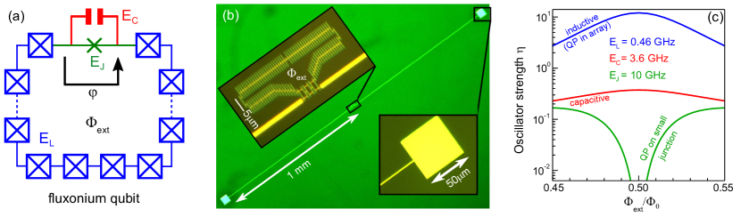
Figure 1: The fluxonium qubit. (a) Electrical circuit schematic. The small junction, which is modeled by an ideal tunnel junction (green) in parallel with a capacitor (red), is shunted by an array of large Josephson junctions (blue). (b) Optical microscope image of the fluxonium qubit inductively coupled to the antenna. The top and bottom insets show magnified images of the fluxonium loop and antenna pads, respectively. The small junction is shunted by a superinductance composed of an array of 95 Josephson junctions, enclosing a magnetic flux $\Phi_{\mathrm{ext}}$. (c) The oscillator strength $\eta$ (see Eq. 1) of different qubit decay mechanisms vs. the applied external flux $\Phi_{\mathrm{ext}}$. The corresponding capacitive, inductive and Josephson energies, defined for the fluxonium artificial atom in Ref. Manucharyan et al. (2009), are shown as $E_{C}$, $E_{L}$ and $E_{J}$ respectively.

The insensitivity of the fluxonium qubit to QP tunneling across the small junction was demonstrated by the measurement of a sharp $T_{1}$ increase to values above $1\>\mathrm{ms}$ in the vicinity of $\Phi_{0}/2$Pop et al. (2014). In addition, non-exponential decay curves were occasionally measured, suggesting a fluctuating QP population. To gain access to these fluctuations, we improved the readout setup used in Ref. Pop et al. (2014) by adding a JPC amplifier, thus increasing the signal-to-noise ratio of the setup by a factor of 10. A schematic of the measurement setup is presented in Fig. 2a.

To monitor the state of the qubit, we apply a continuous wave drive at the cavity resonance corresponding to an average photon population $\bar{n}=2.5$. This value is a compromise between fast measurement and the effect of cavity photons which reduce the qubit lifetime and saturate the JPC outputSup . In Fig. 2b we show a histogram of measured $I,Q$ quadratures at flux bias point $\Phi_{\mathrm{ext}}=\Phi_{0}/2$ where the qubit frequency is $\omega_{ge}/2\pi=665\>\mathrm{MHz}$. The measured distributions corresponding to the ground/excited states of the fluxonium qubit (right/left) are separated by 5 standard deviations $\sigma$. The relative population of the fluxonium in its excited state (33%) corresponds to an effective temperature of 45 mK.

A few examples of measured qubit quantum jump traces are shown in Fig. 2c. To estimate the state of the qubit (orange) from the time trace of quadrature $I$ (blue) we apply a two-point filter. The filter declares a jump in the qubit state if the quadrature value crosses a threshold set $\sigma/2$ away from the jump destination. Otherwise the qubit is declared to remain in its previous state. The traces suggest there are two regimes with distinctly different jump statistics. There appear to be “quiet” times with few jumps and long intervals between them (on the order of 1 ms) and “noisy” times with many rapid consecutive jumps (less than 100 $\mu$s apart).

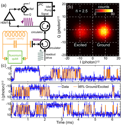
Figure 2: (a) Circuit diagram of the measurement setup. The fluxonium qubit (green) is dispersively coupled to the readout cavity (orange) through the antenna (see Fig. 1b). The readout signal reflected from the cavity is pre-amplified using a JPC, then it is routed through a commercial HEMT amplifier at $4\>\mathrm{K}$ and demodulated using a heterodyne interferometry setup at room temperature. (b) Histogram of measured $I,Q$ quadratures for the fluxonium in equilibrium with its environment at $\Phi_{\mathrm{ext}}=\Phi_{0}/2$ ($\omega_{ge}/2\pi=665\>\mathrm{MHz}$). Each count corresponds to $5\>\mathrm{\mu s}$ of integration and the total number of counts is 200,000. The two distinct peaks in the $I,Q$ plane correspond to the ground (right) and 1st excited (left) states of the qubit. Their relative amplitudes give an effective temperature of $45$ $\mathrm{mK}$. (c) Three examples of measured quantum jump traces corresponding to the time evolution of the $I$ quadrature for the same measurement presented in (b). We show the raw traces in blue and an estimate of the fluxonium qubit state calculated using a two-point filter (see text) in orange. Note that the characteristic time between jumps is not constant throughout the record.

Uncorrelated quantum jumps obey Poisson statistics, leading to an exponential distribution of the time spent in the ground or excited state $p_{\textnormal{\tiny{P}}}(\tau)=\frac{1}{\bar{\tau}}e^{-\tau/\bar{\tau}}$ where $\bar{\tau}$ is the mean time spent in the ground or excited state. To enhance the visibility of deviations from Poisson statistics, which would merely show up as non-exponential decrease of $p(\tau)$, we depict the distribution $\tau p(\tau)$ instead. In Fig. 3a and 3b we show two different second-long measurements of $\tau p(\tau)$ distributions for the ground (blue) and excited (red) states, histogrammed with logarithmic bins. The dashed lines correspond to the distribution predicted by Poisson statistics with $\bar{\tau}$ taken as the measured average time either in the ground (blue) or excited (red) state (see supplementary materialSup for a detailed definition). There is significant deviation between the two measurements. In Fig. 3b we show a measurement record which we call “quiet”, apparently agreeing with Poisson statistics. The “noisy” record in Fig. 3a deviates significantly from the Poisson prediction, with long and short times appearing considerably more frequently than expected.

In Fig. 3c, the mean time spent in the ground (blue) and excited (red) state is shown as a function of time, over several minutes. Each point corresponds to a 1 second temporal average. To quantify the deviation of each measurement from Poisson statistics, we calculate the fidelity of the measured histogram to the Poisson prediction $F=\frac{\sum\limits_{i}\sqrt{M_{i}P_{i}}}{\sum\limits_{i}{M_{i}}}$, where $M_{i}$ is the measured ground state histogram value of bin $i$ and $P_{i}$ is the predicted value of bin $i$ for a Poisson process. In Fig. 3d, we plot the deviation from Poisson statistics, $1-F$, corresponding to the measurements in Fig. 3c. These two figures indicate a correlation between long fluxonium energy lifetimes and agreement with Poisson statisticsSup . The “noisy” seconds appear to have an abundance of short quantum jumps which distort the Poisson statistics, typical for the “quiet” seconds. Fig. 3e shows $\bar{\sigma}_{z}$, the mean polarization of the fluxonium qubit for the same measurements. The fluctuations in polarization are not correlated with the fluctuations between “quiet” and “noisy” seconds. The examples in Fig. 3a and 3b were taken for measurements with the same polarization corresponding to a temperature of $49\>\mathrm{mK}$ (highlighted in gray in Fig. 3c,d,e).

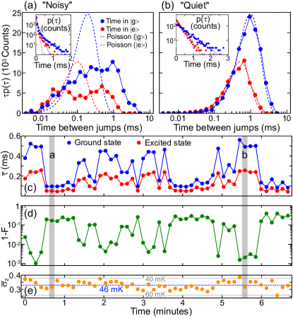
Figure 3: Measurement of “quiet” and “noisy” behavior of the fluxonium quantum jumps. (a,b) Histograms with logarithmic binning of the time intervals between jumps $\tau$ for the qubit in the ground/excited (blue/red) states, scaled by $\tau$. Each count represents a $5\>\mu\mathrm{s}$ time interval. In dashed lines we plot the Poissonian prediction with the measured mean time interval $\bar{\tau}$. Each histogram was taken from a 1 s long measurement record. The insets show the corresponding linear binning histograms proportional to $p(\tau)$. Data in (b) agree with the Poisson prediction, while in (a) significantly deviate from it. (c) Measurement of the average time spent by the qubit in the ground (blue) and excited (red) states vs. time. There are significant fluctuations in these values over the course of minutes. (d) $1-F$ (see text) vs. time, quantifying the deviation between the measured histogram and the corresponding Poisson prediction for the ground state. (e) Average polarization of the fluxonium qubit vs. time. The dashed blue line marks the average polarization which corresponds to a temperature of $46\>\mathrm{mK}$ and the gray dashed lines are markers for $40\>\mathrm{mK}$ and $60\>\mathrm{mK}$. Note that the qubit temperature is not correlated with the fluctuations between the “quiet” and “noisy” intervals.

The susceptibility of the fluxonium qubit at $\Phi_{\mathrm{ext}}=\Phi_{0}/2$ to loss due to QP in the array suggests that fluctuations in the mean time between qubit jumps and their statistics result from the changing QP population. To test this hypothesis, we compare our measurements of spontaneous quantum jump traces to measurements in which we modify the number of QP’s. We do this in two ways: generating QP’s by applying strong microwave pulses and trapping QP’s by cooling in magnetic field.

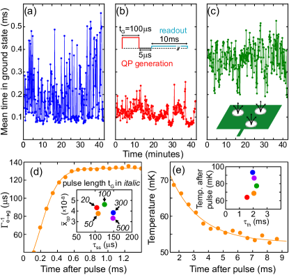
Figure 4: (a) Mean time in the ground state vs. time. Each point represents an average over 1 second. Similar to the data in Fig. 3c, we observe fluctuations between “quiet” and “noisy” intervals. (b) Mean time in the ground state vs. time in the presence of QP generation pulses. The inset shows the pulse sequence we use. A QP generation pulse of length $t_{\textnormal{\tiny{G}}}=100\>\mathrm{\mu s}$ (red) applied at the cavity frequency switches the antenna junctions into the dissipative regime and generates QP in the junction array. This pulse is followed by $5\>\mathrm{\mu s}$ of wait time (black) and a $10\>\mathrm{ms}$ readout pulse (blue) before another QP generation pulse is applied. (c) Mean time in the ground state vs. time, after cooling in magnetic field. (see text). (d) Mean time until a jump from the excited to the ground state vs. time after QP generation pulse of length $t_{\textnormal{\tiny{G}}}=50\>\mathrm{\mu s}$. The solid line is a fit to exponential equilibration of qubit lifetime (see text). The inset shows the saturation relative QP density $\bar{x}_{qp}$ vs. the time to reach steady-state $\tau_{ss}$ for different QP generation pulse lengths. (e) Qubit effective temperature vs. time after QP generation pulse of length $t_{\textnormal{\tiny{G}}}=50\>\mathrm{\mu s}$. The solid line is a fit to an exponential. Inset shows the temperature after a QP generation pulse vs. the thermal equilibration time $\tau_{th}$ for QP generation pulse lengths corresponding to Fig. 4d.

We created a transient QP population in the array by applying a microwave pulse resonant with the cavity frequency of duration $t_{\textnormal{\tiny{G}}}=100\>\mathrm{\mu s}$ and amplitude of order $1$ mV across the antenna, similarly to Ref. Wang et al. (2014). After a $5\>\mathrm{\mu s}$ wait for the cavity photons to leak out, we monitor quantum jumps for $10$ $\mathrm{ms}$, after which we repeat the cycle. We estimate that at least $10^{6}$ QP’s are generated during each pulse. In Fig. 4a and b we show a comparison between measurements of the mean time spent in the ground state without and with QP generation pulses. In the presence of QP generation pulses, the “quiet” seconds (higher mean time in the ground state) are suppressedSup .

We reduced the number of QP’s by cooling down our sample in a constant magnetic field corresponding to $\Phi_{0}/2$ in the fluxonium loop. Under these conditions, the antenna pads (see Fig. 1b) are threaded by flux corresponding to several $\Phi_{0}$. During the field cooldown process the pads can trap vorticesBardeen and Stephen (1965); Stan et al. (2004), which may act as QP traps due to the reduced superconducting gap in their coresUllom et al. (1998); Peltonen et al. (2011); Nsanzineza and Plourde (2014); Wang et al. (2014). Fig. 4c shows measurements of the mean time spent in the ground state taken after the sample was cooled in magnetic field. We observe an increase in the number of “quiet” seconds, indicating a reduction in the number of QP’sSup . The fluxonium effective temperature changes by less than $10\>\mathrm{mK}$ between different cooldowns.

Taking advantage of the real time measurement of the qubit relaxation, we can monitor the time evolution of $\bar{\tau}$ after a QP generation pulse. In Fig. 4d we show the average time spent in the excited state before a jump to the ground state, as a function of time after the QP generation pulse for pulse length $t_{\textnormal{\tiny{G}}}=50\>\mathrm{\mu s}$. This yields the equilibration of qubit lifetime as injected QP’s leave the junction array. The qubit lifetime eventually saturates to a steady state dominated either by non-thermal QP’s or other loss mechanisms. The rate to jump from the excited to the ground state at time $t$ after the pulse is related to the relative QP density byCatelani et al. (2011b):

$$\Gamma_{e\rightarrow g}(t)=x_{qp}(t)\sqrt{\frac{2\Delta}{\hbar\omega_{ge}}}2\pi\frac{E_{L}}{\hbar}$$ (2)

where $x_{qp}$ is the ratio of QP’s to Cooper pairs in the junction array and $\Delta$ is the superconducting gap. We fit the lifetime measurements to an exponential model $x_{qp}(t)=\bar{x}_{qp}+(x_{qp}(0)-\bar{x}_{qp})e^{-t/\tau_{ss}}$ from which we extract the time to reach QP steady-state $\tau_{ss}=125\pm 25\>\mathrm{\mu s}$ and a non-thermal background QP density $\bar{x}_{qp}=4\pm 1\times 10^{-8}$, corresponding to 1-2 QP’s in the whole array. Note that the non-Poissonian jump statistics corresponding to the “noisy” seconds (see Fig. 3a) show fluctuations in the QP number on the order of their average value, also suggesting the presence of only a few QP’s in the whole array. This value for $\bar{x}_{qp}$ is an order of magnitude lower than what was measured for the small junction in Ref. Pop et al. (2014). The origin of the difference is presently not understood, although one could speculate that QP’s in the array more easily diffuse into the antenna. Note that the value for $\bar{x}_{qp}$ is neither correlated with the QP generation pulse length $t_{\textnormal{\tiny{G}}}$ nor the time to reach steady-state $\tau_{ss}$ (see inset of Fig. 4d). The extracted $\bar{x}_{qp}$ should be treated as an upper bound, since contributions from other decay sources could be present. Due to the limited dynamic range of our qubit lifetime measurement, of only a factor of 4, we cannot distinguish between different QP removal mechanisms such as trapping, diffusion or recombinationSup . The discrimination between these mechanisms was recently demonstrated in a transmon qubitWang et al. (2014).

From the quantum jump traces following a QP generation pulse, we can also extract the average polarization of the qubit and hence its effective temperature. In Fig. 4e we show the extracted temperature vs. time, starting from $1.4\>\mathrm{ms}$ after a QP generation pulse, when the QP population has already saturated. The initial increase in temperature following the QP generation pulse is proportional to the pulse length $t_{\textnormal{\tiny{G}}}$, and it is consistent with an estimated dissipated power of $10^{-10}\>\mathrm{W}$ absorbed in the volume of the sapphire substrate. The temperature equilibration time $\tau_{th}$ of several ms is much slower than the sapphire thermalization time and is likely limited by the sapphire-copper contactSup .

In conclusion, the distribution of spontaneous quantum jumps of a fluxonium qubit indicates large relative fluctuations in the energy lifetime of this artificial atom. Corresponding changes of the QP density in the superinductor appear to be the natural explanation. This is supported in particular by the increased fluxonium energy lifetime in the presence of QP trapping vortices, which also render the jump statistics Poissonian. The density of QP’s extracted from the measurement does not appear to self-average over periods of seconds, minutes and even hours. This suggests they originate from sources external to the sample, such as stray infra-redMartinis et al. (2009); Barends et al. (2011) or higher energy radiationSwenson et al. (2010); de Visser et al. (2011). In addition, the fluxonium quantum jump statistics resolves a single QP on a $\mu$s timescale, which could be a useful property for a low flux, low energy, particle counting detector.

We acknowledge fruitful discussions with K. Geerlings and S. M. Girvin. Facilities use was supported by YINQE and NSF MRSEC DMR 1119826. This research was supported by IARPA under Grant No. W911NF-09-1-0369, ARO under Grants No. W911NF-09-1-0514 and W911NF-14-1-0011, NSF under Grants No. DMR-1006060 and DMR-0653377, DOE Contract No. DE-FG02-08ER46482 (LG), and the EU under REA grant agreement CIG-618258 (GC).

References

- Aumentado et al. (2004) J. Aumentado, M. W. Keller, J. M. Martinis, and M. H. Devoret, Physical Review Letters 92, 066802 (2004).
- Ferguson et al. (2006) A. J. Ferguson, S. E. Andresen, R. Brenner, and R. G. Clark, Physical Review Letters 97, 086602 (2006).
- Martinis et al. (2009) J. M. Martinis, M. Ansmann, and J. Aumentado, Physical Review Letters 103, 097002 (2009).
- Shaw et al. (2008) M. D. Shaw, R. M. Lutchyn, P. Delsing, and P. M. Echternach, Physical Review B 78, 024503 (2008).
- de Visser et al. (2011) P. J. de Visser, J. J. A. Baselmans, P. Diener, S. J. C. Yates, A. Endo, and T. M. Klapwijk, Physical Review Letters 106, 167004 (2011).
- Pekola et al. (2008) J. R. Pekola, J. J. Vartiainen, M. Mottonen, O.-P. Saira, M. Meschke, and D. V. Averin, Nature Physics 4, 120 (2008).
- Day et al. (2003) P. K. Day, H. G. LeDuc, B. A. Mazin, A. Vayonakis, and J. Zmuidzinas, Nature 425, 817 (2003).
- Monfardini et al. (2012) A. Monfardini, A. Benoit, A. Bideaud, N. Boudou, M. Calvo, P. Camus, C. Hoffmann, F. X. Desert, S. Leclercq, M. Roesch, et al., Journal of Low Temperature Physics 167, 834 (2012).
- Stone et al. (2012) K. J. Stone, K. G. Megerian, P. K. Day, P. M. Echternach, J. Bueno, and N. Llombart, Applied Physics Letters 100, 263509 (2012).
- Giazotto et al. (2006) F. Giazotto, T. T. Heikkila, A. Luukanen, A. M. Savin, and J. P. Pekola, Reviews of Modern Physics 78, 217 (2006).
- Rajauria et al. (2009) S. Rajauria, H. Courtois, and B. Pannetier, Physical Review B 80, 214521 (2009).
- Bretheau et al. (2013) L. Bretheau, C. O. Girit, H. Pothier, D. Esteve, and C. Urbina, Nature 499, 312 (2013).
- Levenson-Falk et al. (2014) E. M. Levenson-Falk, F. Kos, R. Vijay, L. Glazman, and I. Siddiqi, Physical Review Letters 112, 047002 (2014).
- Lutchyn et al. (2005) R. Lutchyn, L. Glazman, and A. Larkin, Physical Review B 72, 014517 (2005).
- Lenander et al. (2011) M. Lenander, H. Wang, R. C. Bialczak, E. Lucero, M. Mariantoni, M. Neeley, A. D. O’Connell, D. Sank, M. Weides, J. Wenner, et al., Physical Review B 84, 024501 (2011).
- Catelani et al. (2011a) G. Catelani, J. Koch, L. Frunzio, R. J. Schoelkopf, M. H. Devoret, and L. I. Glazman, Physical Review Letters 106, 077002 (2011a).
- Sun et al. (2012) L. Sun, L. DiCarlo, M. D. Reed, G. Catelani, L. S. Bishop, D. I. Schuster, B. R. Johnson, G. A. Yang, L. Frunzio, L. Glazman, et al., Physical Review Letters 108, 230509 (2012).
- Wenner et al. (2013) J. Wenner, Y. Yin, E. Lucero, R. Barends, Y. Chen, B. Chiaro, J. Kelly, M. Lenander, M. Mariantoni, A. Megrant, et al., Phys. Rev. Lett. 110, 150502 (2013).
- Riste et al. (2013) D. Riste, C. C. Bultink, M. J. Tiggelman, R. N. Schouten, K. W. Lenhert, and L. Dicarlo, Nature Communications 4, 1913 (2013).
- Pop et al. (2014) I. M. Pop, K. Geerlings, G. Catelani, R. J. Schoelkopf, L. Glazman, and M. Devoret, Nature 508, 369 (2014).
- Vijay et al. (2011) R. Vijay, D. H. Slichter, and I. Siddiqi, Physical Review Letters 106, 110502 (2011).
- Castellanos-Beltran et al. (2008) M. A. Castellanos-Beltran, K. D. Irwin, G. C. Hilton, L. R. Vale, and K. W. Lehnert, Nature Physics 4, 929 (2008).
- Bergeal et al. (2010) N. Bergeal, F. Schackert, M. Metcalfe, R. Vijay, V. E. Manucharyan, L. Frunzio, D. E. Prober, R. J. Schoelkopf, S. M. Girvin, and M. H. Devoret, Nature 465, 64 (2010).
- Hatridge et al. (2011) M. Hatridge, R. Vijay, D. H. Slichter, J. Clarke, and I. Siddiqi, Physical Review B 83, 134501 (2011).
- Abdo et al. (2013) B. Abdo, A. Kamal, and M. Devoret, Physical Review B 87, 014508 (2013).
- Wang et al. (2014) C. Wang, Y. Y. Gao, I. M. Pop, U. Vool, C. Axline, T. Brecht, R. W. Heeres, L. Frunzio, M. H. Devoret, G. Catelani, et al., arXiv:1406.7300 (2014).
- Manucharyan et al. (2009) V. E. Manucharyan, J. Koch, L. I. Glazman, and M. H. Devoret, Science 326, 113 (2009).
- Manucharyan (2011) V. E. Manucharyan, Ph.D. thesis, Yale University (2011).
- Brooks et al. (2013) P. Brooks, A. Kitaev, and J. Preskill, Physical Review A 87, 052306 (2013).
- Masluk et al. (2012) N. A. Masluk, I. M. Pop, A. Kamal, Z. K. Minev, and M. H. Devoret, Physical Review Letters 109, 137002 (2012).
- (31) See Supplemental Material, which includes Refs. Lecocq et al. (2011); Boissonneault et al. (2008); Slichter et al. (2012); Hatridge et al. (2013); Bhattacharyya (1946); Wilson et al. (2001); Wilson and Prober (2004); Ditmars et al. (1982); Berman et al. (1955).
- Bardeen and Stephen (1965) J. Bardeen and M. J. Stephen, Physical Review 140, 1197 (1965).
- Stan et al. (2004) G. Stan, S. B. Field, and J. M. Martinis, Physical Review Letters 92, 097003 (2004).
- Ullom et al. (1998) J. N. Ullom, P. A. Fisher, and M. Nahum, Applied Physics Letters 73, 2494 (1998).
- Peltonen et al. (2011) J. T. Peltonen, J. T. Muhonen, M. Meschke, N. B. Kopnin, and J. P. Pekola, Physical Review B 84, 220502 (2011).
- Nsanzineza and Plourde (2014) I. Nsanzineza and B. L. T. Plourde, Physical Review Letters 113, 117002 (2014).
- Catelani et al. (2011b) G. Catelani, R. J. Schoelkopf, M. H. Devoret, and L. I. Glazman, Physical Review B 84, 064517 (2011b).
- Barends et al. (2011) R. Barends, J. Wenner, M. Lenander, Y. Chen, R. C. Bialczak, J. Kelly, E. Lucero, P. O’Malley, M. Mariantoni, D. Sank, et al., Applied Physics Letters 99, 113507 (2011).
- Swenson et al. (2010) L. J. Swenson, A. Cruciani, A. Benoit, M. Roesch, C. S. Yung, A. Bideaud, and A. Monfardini, Applied Physics Letters 96, 263511 (2010).
- Lecocq et al. (2011) F. Lecocq, I. M. Pop, Z. Peng, I. Matei, T. Crozes, T. Fournier, C. Naud, W. Guichard, and O. Buisson, Nanotechnology 22, 315302 (2011).
- Boissonneault et al. (2008) M. Boissonneault, J. M. Gambetta, and A. Blais, Physical Review A 77, 060305 (2008).
- Slichter et al. (2012) D. H. Slichter, R. Vijay, S. J. Weber, S. Boutin, M. Boissonneault, J. M. Gambetta, A. Blais, and I. Siddiqi, Physical Review Letters 109, 153601 (2012).
- Hatridge et al. (2013) M. Hatridge, S. Shankar, M. Mirrahimi, F. Schackert, K. Geerlings, T. Brecht, K. M. Sliwa, B. Abdo, L. Frunzio, S. M. Girvin, et al., Science 339, 178 (2013).
- Bhattacharyya (1946) A. Bhattacharyya, Sankhya 7, 401 (1946).
- Wilson et al. (2001) C. M. Wilson, L. Frunzio, and D. E. Prober, Physical Review Letters 87, 067004 (2001).
- Wilson and Prober (2004) C. M. Wilson and D. E. Prober, Physical Review B 69, 094524 (2004).
- Ditmars et al. (1982) D. A. Ditmars, S. Ishihara, S. S. Chang, G. Bernstein, and E. D. West, Journal of Research of the National Bureau of Standards 87, 159 (1982).
- Berman et al. (1955) R. Berman, E. L. Foster, and J. M. Ziman, Proceedings of the Royal Society of London Series A-mathematical and Physical Sciences 231, 130 (1955).