Constraining the nuclear energy density functional with quantum Monte Carlo calculations

Abstract

We study the problem of an impurity in fully polarized (spin-up) low density neutron matter with the help of an accurate quantum Monte Carlo method in conjunction with a realistic nucleon-nucleon interaction derived from chiral effective field theory at next-to-next-to-leading-order. Our calculations show that the behavior of the proton spin-down impurity is very similar to that of a polaron in a fully polarized unitary Fermi gas. We show that our results can be used to put tight constraints on the time-odd parts of the energy density functional, independent of the time-even parts, in the density regime relevant to neutron-rich nuclei and compact astrophysical objects such as neutron stars and supernovae.

Introduction.— The ab initio prediction of nuclear properties from quantum chromodynamics (QCD) remains an unresolved challenge in fundamental science. Its importance extends well beyond the confines of basic nuclear physics, into the realm of astrophysics, viz. in the physics of neutron stars and core-collapse supernovae.

It is unlikely that direct lattice QCD calculations of many hadron properties will be possible in the forseeable future. However, in the past two decades a promising alternative route has been proposed and pursued with vigor. This scheme consists of bridging the gap between QCD and low energy nuclear physics by building successive effective theories.

In the first step one constructs an effective Hamlitonian with the hadronic degrees of freedom. The structure of this Hamiltonian is tightly constrained by chiral effective field theory (EFT) Epelbaum et al. (2009); *Machleidt2011; *Hammer2013. In the next stage one performs accurate many body calculations with this effective Hamiltonian for simple configurations, e.g. homogeneous matter, light and medium mass nuclei etc. Results from these calculations, in conjunction with experimental data, are eventually used to construct an energy density functional (EDF) for nuclear systems. Density functional theory is, presently, the only viable computational method for complex inhomogeneous systems.

It is of paramount importance that the effective theory at each stage is consistent with the available experimental data and the predictions of the underlying microscopic theory. A successful prototype is provided by the density functional theory for electronic structure calculations Perdew and Wang (1992) which was fit to accurate quantum Monte Carlo (QMC) calculations for the electron gas Ceperley and Alder (1980). Of course, nuclear systems are far more complicated because of the complexity of the nuclear forces and the remaining ambiguities in their short range structure.

Most nuclear EDFs are fit to the ground state properties of even-even nuclei, saturation properties of nuclear matter and occasionally to microscopic calculations of unpolarized neutron matter. These quantities constrain only that part of the EDF which depends on the time-reversal-even densities (“time-even part”). The EDF also depends on time-reversal-odd densities (“time-odd part”) which plays an important role in a variety of phenomena: binding energies of odd-mass nuclei Satula , pairing correlations in nuclei Duguet et al. (2001), distribution of the Gamow-Teller strength Bender et al. (2002), properties of rotating nuclei Dobaczewski and Dudek (1995); *Post1985, nuclear magnetism Afanasjev and Ring (2000) etc. At present, the time-odd part of the Skyrme and other non–relativistic nuclear EDF is ill-determined because of the lack of unambiguous constraints from experiment or ab–initio calculations.

In the recent past, there is an emerging consensus that the theoretical uncertainities of the nuclear forces is largely suppressed in low density neutron matter (densities sufficiently less than the saturation density of nuclear matter). In this regime, the properties of the relevant components of the two nucleon forces are well established and the contributions from three and higher body forces are rather small. Any realistic nucleon-nucleon interaction, which fits the low energy nucleon-nucleon scattering phase shifts and the binding energy of deuteron, in conjunction with an accurate many body method produce consistent “theoretical data”; which can provide constraints for the EDF complementary to those coming from experiments.

In this paper we report the results from fully non-perturbative QMC calculations with a chiral EFT Hamiltonian for fully polarized (spin up) low density neutron matter with an impurity (spin down neutron or spin up/down proton). The impurity problem that we discuss here is a generalization of the well known polaron problem in solid state systems and in ultracold gases (see, e.g. in Chevy and Mora (2010); *Massignan2014). In fact, we find that the proton spin-down impurity behaves in a manner which is qualitatively very similar to a polaron in a fully polarized Fermi gas in the unitary regime, i.e., the regime with diverging s-wave scattering length ($a_{s}\to\infty$) and vanishing effective range ($r_{e}\to 0$), over a wide density range $10^{-3}\mbox{ fm}^{-3}\leq\rho\leq 5\times 10^{-2}\mbox{ fm}^{-3}$.

We show that the difference between energies of the proton spin up and spin down impurities depends only on the time-odd part of the EDF. Thus, our results provide stringent constraints for the time-odd part of the density functional, independent of the time-even part. The results presented here will provide valuable guidance in constructing EDFs in regimes relevant to neutron-rich nuclei, neutron star crusts and supernovae neutrinosphere.

Method.— Our calculations are based on the recently developed QMC method called the configuration interaction Monte Carlo (CIMC) method Mukherjee and Alhassid (2013); Roggero et al. (2013, 2014). The CIMC method is based on filtering out an eigenstate $\Psi_{0}$ of the Hamiltonian $H$ by repeated application of the propagator $\mathcal{P}=e^{-\tau(H-E_{T})}$ on an initial state $\Psi_{\rm I}$,

$$|\Psi_{0}\rangle=\lim_{\mathcal{N}_{\tau}\to\infty}\mathcal{P}^{\mathcal{N}_{\tau}}|\Psi_{\rm I}\rangle.$$ (1)

Here, $E_{T}$ is an energy shift used to keep the norm of the wave function approximately constant, and $\tau$ is a finite step in ‘imaginary’ time $\tau=it$. The state, $\Psi_{0}$, is the eigenstate with the lowest eigenvalue within the subset of states having non-zero overlaps with $\Psi_{\rm I}$.

The application of the propagator is carried out stochastically. The main difference between the CIMC method and traditional continuum diffusion Monte Carlo methods is that in the CIMC method this stochastic projection is performed in Fock space ( i.e. the basis is provided by the Slater determinants that can constructed from a finite set of single particle (sp) basis states), as opposed to the coordinate space. As a result, non-local Hamiltonians do not pose any technical problems.

In this work, we use the sp basis given by eigenstates of momentum and the $z$ components of spin and isospin. The calculations for fully polarized neutrons are performed in a box containing $N$ spin-up neutrons. The impurity system contains an additional impurity particle. Periodic boundary conditions are imposed. The size of the box is given by the density, $\rho$, of the spin-up neutrons, $L^{3}=N/\rho$. The finite size of the box implies that the sp states are restricted to a lattice in momentum space with a lattice constant $l=2\pi/L$.

A finite sp basis is chosen by imposing a “basis cutoff” $k_{\rm max}$, so that only those sp states with $\mathbf{k}^{2}\leq k_{\rm max}^{2}$ are included. A sequence of calculations, with successively larger values of $k_{\rm max}$, are performed till convergence is reached. We deem the calculations to have converged in $k_{\rm max}$ when the difference in the energies between the successive calculations are smaller than the statistical error ($\sim 10$ KeV ).

Sampling of new states can be performed under the condition that the matrix elements of the propagator, $\mathcal{P}$, are always positive semi-definite. For fermions interacting via realistic potentials, this condition is never fullfilled. (An interesting exception is provided by the pure pairing Hamiltonian Cerf and Martin (1993); *Mukherjee2011.) This gives rise to the so-called sign-problem, which we circumvent by using a guiding wave function to constrain the random walk to a subsector of the full many-body Hilbert space in which the sampling procedure is well defined Mukherjee and Alhassid (2013). This restriction of the random walk introduces an approximation which is similar to the fixed-node/fixed-phase approximation commonly used in continuum QMC. Our method provides strict variational upper bounds for the energy.

As explained in Refs. Roggero et al., 2013, 2014, we use coupled cluster double (CCD) type wave functions as the guiding wave functions. As a result, the CIMC method provides an interesting synthesis of QMC methods and coupled cluster (CC) theory. In principle, the fixed phase approximation can be systematically improved by including irreducible triples, quadrupoles etc. in the guiding wave function. However, as discussed in Ref. Roggero et al., 2014 these contributions are expected to be rather small at these densities (less than a few percent of the total correlation energy).

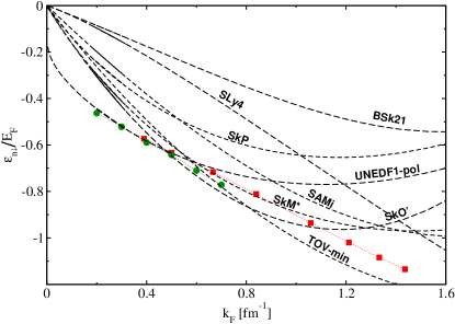
Figure 1: (Color online) The energy of the neutron spin-down impurity in the units of the Fermi energy of the spin-up neutrons. The red filled squares are our QMC results with the NNLO_opt interaction. The green filled circles are the GFMC calculations with an s-wave interaction fit to the $nn$ scattering length and effective range Forbes et al. (2014). The black dashed lines are predictions from various density functionals (see text).

Results.— We calculate the ground state energies for a fully polarized system and that with an additional impurity particle. The difference between these two energies gives the impurity energy. We use the recently developed next-to-next-to-leading order chiral NNLO_opt interaction Ekström et al. (2013) for our calculations. The scattering phase shifts obtained from this interaction fit the experimental database Stoks et al. (1993) at $\chi^{2}\sim 1$ for laboratory energies less than $125$ MeV. However, as alluded to in the introduction, the conclusions we present are independent of the particular interaction model we are using.

In Fig. 1 we plot the ratio of the energy of neutron spin-down impurity, $\varepsilon_{n\downarrow}$, and the Fermi energy of the fully polarized system, $E_{F}$, versus the Fermi momentum $k_{F}$. Our results are good agreement with the GFMC calculations reported in Ref. Forbes et al., 2014 using an s-wave interaction (fit to the $nn$ scattering length and effective range). For example, at $k_{F}=0.4$ fm^-1, we get $\varepsilon_{n\uparrow}/E_{F}=-0.582\pm 0.002$ while the GFMC calculation gives $-0.589\pm 0.005$. An AFDMC calculation performed the Argonne $v_{8}^{\prime}$ potential gives $-0.567\pm 0.006$ at the same $k_{F}$.

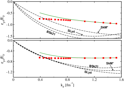
Figure 2: (Color online) The energy of the proton spin-up (top panel) and spin-down (bottom panel) impurities in the units of the Fermi energy of the spin-up neutrons. The red filled squares are our QMC results with the NNLO_opt. interaction. The green solid lines are the results from second order perturbation theory. The black dashed lines are predictions from various density functionals (see text).

The impurity energies reported in Fig. 1 and later in Fig. 2 were performed with $N=7$ spin-up neutrons. We have checked in selected cases that the difference between the $N=7$ and the $N=33$ energies is about $1-2$%. For example, for $\rho=0.04$ fm^-3 $\varepsilon_{n\downarrow}/E_{F}$ is $-0.6698\pm 0.0005$ with $N=7$ and is $-0.664\pm 0.006$ for $N=33$, while for $\rho=0.06$ fm^-3 the corresponding values are $-0.6617\pm 0.0003$ and $-0.647\pm 0.004$. With $N=7$ the size of the box, $L$, for the largest density we consider in this work ($\rho=0.06$ fm^-3) is about $4.9$ fm. This is about three times the characteristic range of the nucleon-nucleon interaction given by the pion Compton wavelength ($\approx 1.4$ fm). At higher densities ($\rho\geq 0.16$ fm^-3) the corrections resulting from performing calculations with a finite number of particles is expected to sizeable and it is customary to perform calculations with larger particle number ($N\geq 33$, for each spin). However, at the densities we are considering in this paper, the finite particle number corrections (even at $N=7$) can be reasonably expected to be smaller than, or at most comparable to, the other sources of uncertainty (the non inclusion of three body forces in the Hamiltonian or the absence of triples in the wave function).

In Fig. (2) we plot the ratio of the energy of the proton spin up/down impurity ($\varepsilon_{p\uparrow/\downarrow}$) and $E_{F}$. The density dependence of $\varepsilon_{p\uparrow/\downarrow}/E_{F}$ is rather weak. In fact, the QMC results for $\varepsilon_{p\downarrow}/E_{F}$ change by less than $2\%\;(-0.681<\varepsilon_{p\downarrow}/E_{F}<-0.666)$ when the density changes by more than an order of magnitude ($10^{-3}-5\times 10^{-2}$). Interestingly, this value is larger, in magnitude, than the corresponding (theoretical) value for polaron energy in a fully polarized unitary Fermi gas ($\approx-0.6$) Lobo et al. (2006); *Prokofev2008 by about $10\%$. It is worth pointing out here that the singlet $pn$ scattering length is about $25\%$ larger than the singlet $nn$ scattering length. This weak density dependence of $\varepsilon_{p\uparrow/\downarrow}$ is a non-perturbative result. Calculations from second order perturbation theory, also shown in the figure, predict a much stronger density dependence for $k_{F}<1.0$ fm.

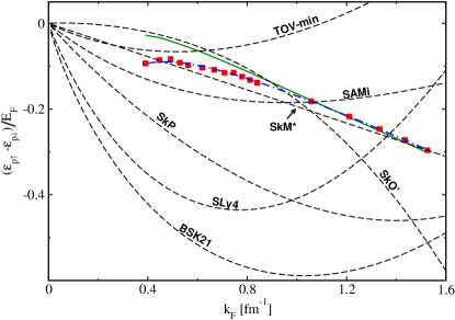
Figure 3: (Color online) The difference between the energies of the proton spin-up and spin-down impurities in the units of the Fermi energy of the spin-up neutrons. The red filled squares are our QMC results with the chiral NNLO_opt interaction. The green solid line is the prediction from second order perturbation theory. The blue dot-dashed line is a fit of the form : $A-\frac{B}{k_{F}|a_{s}|}-Ck_{F}r_{e}$. The black dashed lines are predictions from various density functionals (see text).

The Skyrme EDF for uniform matter is usually parametrized as

$$\mathcal{E}=\mathcal{E}_{\rm kin}+\sum_{t=0,1}\left(C^{\rho}_{t}\rho_{t}^{2}+C^{\tau}_{t}\rho_{t}\tau_{t}+C^{s}_{t}s_{t}^{2}+C^{T}_{t}s_{t}T_{t}\right).$$ (2)

where $\mathcal{E}_{\rm kin}$ is the kinetic energy density. The isoscalar (isovector) density, spin-density, kinetic density and spin-kinetic density are denoted by $\rho_{0},s_{0},\tau_{0}$ and $T_{0}$ ($\rho_{1},s_{1},\tau_{1}$ and $T_{1}$ ), respectively. The part of the density functional which explicitly depends on the time-odd densities ($s_{t}$, $T_{t}$) is the time-odd part, and the rest is the time-even part.

The coefficients $C^{\rho}_{t},C^{\tau}_{t},C^{s}_{t}$ and $C^{T}_{t}$ can only depend on the total (isoscalar) density $\rho_{0}=\rho$. In general, the coefficients are all independent and should be fixed from available data. However, for EDFs derived from a Skyrme force, there are additional relationships amongst the coefficients and the number of indepedent coefficients is smaller. Usually the $C^{\rho}_{t}$ and $C^{s}_{t}$ are assumed to have the form

$$C^{(\rho/s)}_{t}=C^{(\rho/s)0}_{t}+C^{(\rho/s)\rho}_{t}\rho^{(\gamma/\delta)}.$$ (3)

The impurity energy can be calculated from the EDF as

$$\varepsilon_{\tau\sigma}=\left.\frac{\partial\mathcal{E}}{\partial\rho_{\tau\sigma}}\right|_{\rho_{\tau\sigma}\to 0},$$ (4)

with $\tau\sigma=\{n\downarrow,p\uparrow,p\downarrow\}$. In Fig. (1) we also show $\varepsilon_{n\downarrow}/E_{F}$ obtained from a wide cross-section of currently popular EDFs: SLy4 Chabanat et al. (1995); *Chabanat1997; *Chabanat1998, SkM* Bartel et al. (1982), BSk21 Goriely et al. (2010), SkP Dobaczewski et al. (1984), SkO^′ Reinhard et al. (1999), SAMi Roca-Maza et al. (2012), TOV-min Erler et al. (2013) and UNEDF-pol Forbes et al. (2014). In Fig. 2, we show $\varepsilon_{p\uparrow/\downarrow}/E_{F}$ for a smaller sub-section of the EDFs. This is done in order to avoid over-crowding the figure. However, we would like to note here that the three EDFs, which are plotted in Fig. 2, provide a fair representation of the spread in the predictions from the current Skyrme–type EDFs; all the other EDFs show very similar trends both qualitatively and quantitatively.

None of the EDFs reproduce the QMC results satisfactorily. This is even more evident in the case of the proton spin-down impurity; whereas all the EDFs predict $\varepsilon_{p\downarrow}/E_{F}$ to be decreasing with $k_{F}$, our QMC calculations predict a flat behavior. This is not unexpected since the EDFs are usually fit to the experimental properties nuclear systems near saturation density and low isospin polarization (stable nuclei), and many body calculations of unpolarized neutron matter. On the basis of our calculations we conclude that in order to account for the correlations in the low density matter in the presence of large spin and isospin polarization, qualitative changes are warranted in the form of the EDFs.

The difference $\varepsilon_{p\uparrow}-\varepsilon_{p\downarrow}$ is a purely time-odd quantity. From Eqs. (2) and (4) one can easily obtain the following relation

$$\frac{\varepsilon_{p\uparrow}-\varepsilon_{p\downarrow}}{E_{F}}=\frac{4m(C^{s}_{0}-C^{s}_{1})}{3\pi^{2}\hbar^{2}}k_{F}-\frac{2m(C^{T}_{0}-C^{T}_{1})}{5\pi^{2}\hbar^{2}}k_{F}^{3}.$$ (5)

In Fig.(3) we compare the predictions from our QMC calculations for $(\varepsilon_{p\uparrow}-\varepsilon{p\downarrow})/E_{F}$ with those from different EDFs. It is clear that none of the EDFs correctly describe our results. The SkM* EDF reproduces the linear part of our results reasonablly well. However, the SkM* EDF does not perform any better than the other EDFs for the individual $\varepsilon_{p\uparrow/\downarrow}$. Also, globally the SkM* EDF fares significantly worse than the more modern EDFs in describing experimental data for nuclei (e.g., masses).

Our results are well fit by the form

$$\frac{\varepsilon_{p\uparrow}-\varepsilon_{p\downarrow}}{E_{F}}=A-\frac{B}{k_{F}|a_{s}|}-Ck_{F}r_{e}$$ (6)

with $A=0.17\pm 0.01$, $B=1.4\pm 0.1$ and $C=0.101\pm 0.001$. We have used the values $a_{s}=-23.75$ fm and $r_{e}=2.75$ fm for the neutron-proton singlet scattering length and effective length, respectively. This form is clearly reminscent of a dilute unitary Fermi gas.

Conclusion.— We have presented QMC calculations with a chiral interaction for the impurities in low density fully polarized neutron matter. The proton spin-down impurity shows universal behaviour for a wide range of densities. None of the state of the art Skyrme EDFs describe our microscopic calculations correctly. We showed that the difference between the proton impurity energies depends only on the time-odd part of the EDF. We found a simple functional form which fits our results for this difference, but is nevertheless qualitatively different from what is predicted by the current functional forms used in the Skyrme EDFs. Our results provide new constraints for constructing accurate density functionals.

Acknowledgments..— We thank A. Gezerlis for sharing the results of their numerical simulations. The authors are also members of LISC, the Interdisciplinary Laboratory for Computational Science, a joint venture between Fondazione Bruno Kessler and the University of Trento. Computations have been carried out mostly on the open facilities at Lawrence Livermore National Laboratory.

References

- Epelbaum et al. (2009) E. Epelbaum, H. W. Hammer, and U. G. Meißner, Rev. Mod. Phys. 81, 1773 (2009).
- Machleidt and Entem (2011) R. Machleidt and D. R. Entem, Phys. Rep. 503, 1 (2011).
- Hammer et al. (2013) H. W. Hammer, A. Nogga, and A. Schwenk, Rev. Mod. Phys. 85, 197 (2013).
- Perdew and Wang (1992) J. P. Perdew and Y. Wang, Phys. Rev. B 45, 13244 (1992).
- Ceperley and Alder (1980) D.M. Ceperley and B.J. Alder, Phys. Rev. Lett. 45, 566 (1980).
- (6) W. Satula, in Nuclear Structure’98, AIP Conf. Proc. No. 481 (AIP, New York, 1999), edited by C. Baktash, p. 114.
- Duguet et al. (2001) T. Duguet, P. Bonche, P. H. Heenen, and J. Meyer, Phys. Rev. C 65, 014310 (2001).
- Bender et al. (2002) M. Bender, J. Dobaczewski, J. Engel, and W. Nazarewicz, Phys. Rev. C 65, 054322 (2002).
- Dobaczewski and Dudek (1995) J. Dobaczewski and J. Dudek, Phys. Rev. C 52, 1827 (1995).
- Post et al. (1985) U. Post, E. Wüst, and U. Mosel, Nucl. Phys. A437, 274 (1985).
- Afanasjev and Ring (2000) A. V. Afanasjev and P. Ring, Phys. Rev. C 62, 031302 (2000).
- Chevy and Mora (2010) F. Chevy and C. Mora, Rept. Prog. Phys. 73, 112401 (2010).
- Massignan et al. (2014) P. Massignan, M. Zaccanti, and G. M. Bruun, Reports on Progress in Physics 77, 034401 (2014).
- Mukherjee and Alhassid (2013) A. Mukherjee and Y. Alhassid, Phys. Rev. A 88, 053622 (2013).
- Roggero et al. (2013) A. Roggero, A. Mukherjee, and F. Pederiva, Phys. Rev. B 88, 115138 (2013).
- Roggero et al. (2014) A. Roggero, A. Mukherjee, and F. Pederiva, Phys. Rev. Lett. 112, 221103 (2014), arXiv:1402.1576 [nucl-th] .
- Cerf and Martin (1993) N. Cerf and O. Martin, Phys. Rev. C 47, 2610 (1993).
- Mukherjee et al. (2011) A. Mukherjee, Y. Alhassid, and G.F. Bertsch, Phys. Rev. C 83, 014319 (2011).
- Forbes et al. (2014) M.M. Forbes, A. Gezerlis, K. Hebeler, T. Lesinski, and A. Schwenk, Phys. Rev. C 89, 041301(R) (2014).
- Ekström et al. (2013) A. Ekström, G. Baardsen, C. Forssén, G. Hagen, M. Hjorth-Jensen, G. R. Jansen, R. Machleidt, W. Nazarewicz, T. Papenbrock, J. Sarich, and S. M. Wild, Phys. Rev. Lett. 110, 192502 (2013).
- Stoks et al. (1993) V. G. J. Stoks, R. A. M. Klomp, M. C. M. Rentmeester, and J. J. de Swart, Phys. Rev. C 48, 792 (1993).
- Lobo et al. (2006) C. Lobo, A. Recati, S. Giorgini, and S. Stringari, Phys. Rev. Lett. 97, 200403 (2006).
- Prokof’ev and Svistunov (2008) N. Prokof’ev and B. Svistunov, Phys. Rev. B 77, 020408 (2008).
- Chabanat et al. (1995) E. Chabanat, P. Bonche, P. Haensel, J. Meyer, and R. Schaeffer, Physica Scripta 1995, 231 (1995).
- Chabanat et al. (1997) E. Chabanat, P. Bonche, P. Haensel, J. Meyer, and R. Schaeffer, Nucl. Phys. A627, 710 (1997).
- Chabanat et al. (1998) E. Chabanat, P. Bonche, P. Haensel, J. Meyer, and R. Schaeffer, Nucl. Phys. A635, 231 (1998).
- Bartel et al. (1982) J. Bartel, P. Quentin, M. Brack, C. Guet, and H.-B. Håkansson, Nucl. Phys. A386, 79 (1982).
- Goriely et al. (2010) S. Goriely, N. Chamel, and J.M. Pearson, Phys. Rev. C 82, 035804 (2010).
- Dobaczewski et al. (1984) J. Dobaczewski, H. Flocard, and J. Treiner, Nucl. Phys. A422, 103 (1984).
- Reinhard et al. (1999) P. G. Reinhard, D. J. Dean, W. Nazarewicz, J. Dobaczewski, J. A. Maruhn, and M. R. Strayer, Phys. Rev. C 60, 014316 (1999).
- Roca-Maza et al. (2012) X. Roca-Maza, G. Colo, and H. Sagawa, Physical Review C 86, 031306 (2012).
- Erler et al. (2013) J. Erler, C.J. Horowitz, W. Nazarewicz, M. Rafalski, and P.-G. Reinhard, Phys. Rev. C 87, 044320 (2013).