Precision of future experiments measuring primordial tensor fluctuation

Abstract

Recently the second phase of Background Imaging of Cosmic Extragalactic Polarization (BICEP2) claimed a detection of the tensor-to-scalar ratio ($r$) of primordial fluctuation at $5\sigma$ confidence level. If it is true, this large and measurable amplitude ($r\simeq 0.2$) of B-mode polarization indicates that it is possible to measure the shape of CMB B-mode polarization with future experiments. We forecast the precision of $r$ and the tensor spectral index $n_{\rm t}$ measurements, with $n_{\rm t}$ as a free parameter, from a Planck-like experiment, and from Spider and POLARBEAR given the current understanding of their experimental noise and foreground contamination. We quantitatively determine the signal-to-noise of the measurement in $r$-$n_{\rm t}$ parameter space for the three experiments. The forecasted signal-to-noise ratio of the B-mode polarization somewhat depends on $n_{\rm t}$, but strongly depends on the true value of $r$.

Introduction– Recently the BICEP2 experiment claimed a more than $5\sigma$ detection of CMB B-mode polarization BICEP2 . This detection, if confirmed by ongoing and forthcoming experiments, implies a large amplitude of primordial tensor fluctuations and therefore has profound theoretical implications. For instance, given the current detected amplitude $r=0.2$, the inflationary potential and the associated derivatives can be completely reconstructed around a few number of e-folds Ma:2014vua . However, on the other hand, several other groups claimed recently that the BICEP2 results may come from the spurious signal of the polarized dust Flauger14 .

Assuming the BICEP2 result is correct and therefore the primordial tensor fluctuation is measurable, it is possible to measure not only the amplitude but also the shape of the primordial tensor power spectrum with future experiment. The BICEP2 measured B-mode power spectrum has power excess at small scales, indicating a blue tilt ($n_{\rm t}$) of the spectrum . The statistical significance of such a blue tensor spectrum is found to be in between $1\sigma$ and $2\sigma$ Gerbino:2014eqa ; Wang:2014kqa .

The hint of blue $n_{\rm t}$ becomes stronger when the BICEP2 data is combined with Wilkinson Microwave Anisotropy Probe (WMAP) and Planck data Wang:2014kqa ; Ashoorioon:2014nta ; Smith:2014kka . In fact, before the tensor mode is detected, the theoretical prediction of temperature power spectrum is around $5\%$–$10\%$ higher than the measurement on $\ell<50$ Ade:2013kta . The detected tensor-to-scalar ratio $r=0.2$ will further enhance the low-$\ell$ temperature power spectrum ($C^{\rm TT}_{\ell}$) by $10\%$ since the primordial gravitational wave preserves only on very large scales. This ensures that the standard model even more inconsistent with the observational data.

The possibility of a blue power spectrum with positive $n_{\rm t}$ can reconcile the tension between model and the data. With positive $n_{\rm t}$, the contribution to $C^{\rm TT}_{\ell}$ ($\ell<50$) is less than red tensor spectrum, making the model prediction more consistent with the data Liu04 . It has been shown that once $n_{\rm t}$ is released to be a free parameter in the likelihood analysis, a positive $n_{\rm t}$ is found to be at $3\sigma$ confidence level (CL) Smith:2014kka ; Cai:2014hja . A similar hint for a blue power spectrum is also found in the results of global fittings Wu:2014qxa ; Li:2014cka .

Given the current BICEP2 constraints on $r$ and $n_{\rm t}$, in this paper we will investigate how precisely the on-going and future experiments can measure these two parameters and therefore determine the tensor spectrum. Specifically, we will forecast the precision of measurement from a Planck-like full-sky CMB experiment , and from the Spider Crill08 and POLARBEAR PolarBear experiments with the current understanding of their experimental noise and foreground contamination.

The primordial tensor power spectrum can be expanded in power law form:

$$P_{\rm t}(k)=A_{\rm t}(k_{0})\left(\frac{k}{k_{0}}\right)^{n_{\rm t}},$$ (1)

where $k_{0}$ is the pivot wave number at which $n_{\rm t}$ and $A_{\rm t}$ are evaluated. The amplitude of tensor power spectrum, $A_{\rm t}(k_{0})$ is related to the tensor-to-scalar ratio as given by

$$r=\frac{A_{\rm t}(k_{0})}{A_{\rm s}(k_{0})},$$ (2)

where $A_{\rm s}(k_{0})$ is the scalar amplitude at $k_{0}$. In our data analysis, we use $k_{0}=0.01\,{\rm Mpc}^{-1}$. Then the power spectrum $C_{\ell}^{\rm BB}$ is related to $P_{\rm t}(k)$ by

$$C_{\ell}^{\rm BB}=\frac{\pi}{4}\int P_{\rm t}(k)\Delta_{\ell}^{\rm B}(k)^{2}{\rm d}\ln k,$$ (3)

where $\Delta^{\rm B}_{\ell}(k)$ is the transfer function for each multipole $\ell$ which can be obtained from public code camb cambcode .

Constraining $r$ and $n_{\rm t}$ from BICEP2 and Planck data– Here we make use of the public code CosmoMC Lewis:2002ah to constraint $r$ and $n_{\rm t}$. The other cosmological parameters are fixed at the best-fitting value from Planck. With BICEP2 data and marginalizing over $r$, we can obtain the likelihood on $n_{\rm t}$ as $1.24\pm 0.90$ ($1\sigma\,$ CL). By combining BICEP2 data with Planck (2013) and WMAP polarization (WP) data, we find $n_{\rm t}=1.76\pm 0.54$ ($1\sigma\,$ CL). When marginalizing over $n_{\rm t}$, the likelihood on $r$ are $r=0.20\pm 0.06$ and $r=0.18\pm 0.05$ at $1\sigma$ CL for BICEP2 only and BICEP2+Planck (2013)+WP, respectively. The $1\sigma$ and $2\sigma$ contours are plotted on Figure 1, where the blue contours are for BICEP2 only, and the red contours are for BICEP2+Planck (2013)+WP. It is worth noting that the inclusion of Planck (2013)+WP does not change the contour significantly at large positive $n_{\rm t}$ part, but it sets strong limit on small $n_{\rm t}$. Therefore, the negative $n_{\rm t}$ (red tilted power spectrum) is disfavored at more than $3\sigma\,$CL. This is clearly inconsistent with the consistency relation of the single-field slow-roll inflation where $n_{\rm t}$ is slightly negative given the current measurement of $r$. If the positive $n_{\rm t}$ is found to be true, this clearly indicates some new physics for inflation.

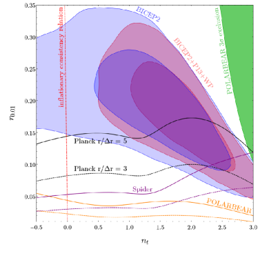
Figure 1: Signal-to-noise ratio of Planck (black lines), Spider (purple lines) and POLARBEAR (orange lines) as functions of $r$ and $n_{\rm t}$. Solid lines denote signal-to-noise ratio $r/\Delta r=5$ and the dashed lines denote signal-to-noise ratio $r/\Delta r=3$. Current observations are also plotted. Blue contours are the $1\sigma$ and $2\sigma$ constraints from BICEP2. Red contours are the combined constraints from BICEP2+Planck (2013)+WMAP polarization (WP). Current POLARBEAR $3\sigma$ exclusion region is plotted in green. Nearly vertical red dash-dotted line is the consistency relation $r=-8n_{\rm t}$ predicted by the minimal model of inflation.

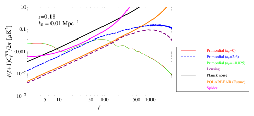
Figure 2: Comparison between B-mode polarization power spectra of models with $n_{\rm t}=0$ (flat power spectrum), $n_{\rm t}=-r/8=-0.025$ (consistency relation) and $n_{\rm t}=2.6$ ($2\sigma$ upper limit of current constraint) and noise level for Planck, Spider and POLARBEAR experiments. Purple dashed line is the B-mode signal induced by gravitational lensing (non-primordial).

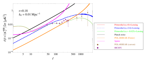
Figure 3: Comparison between the total B-mode polarization power spectra (primordial plus lensing) of the same three models as described previously and noise level for Planck, Spider and POLARBEAR experiments. Brown and purple data with error-bars are the band-power data from the current experiments.

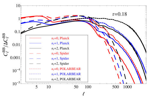
Figure 4: Signal to noise ($\Delta C_{\ell}^{\rm BB}$ is calculated through eq. (4)) at each $\ell$ for Planck (solid lines), Spider (long-dashed lines) and POLARBEAR (short-dashed lines). Value of $n_{\rm t}$ is taken to be $0$ (red), $1$ (blue) and $2$ (black). Value of $r$ is fixed to be $0.18$ at pivot scale $k_{0}=0.01\,{\rm Mpc}^{-1}$.

Model	Experiment	$\ell\leq 100$	$100<\ell<3000$
	Planck	7.57	1.98
$n_{\rm t}=0$	Spider	14.89	4.18
	POLARBEAR	8.41	6.59
	Planck	5.65	2.72
$n_{\rm t}=1$	Spider	12.87	5.28
	POLARBEAR	8.27	9.64
	Planck	5.87	5.70
$n_{\rm t}=2$	Spider	13.48	8.55
	PPOLARBEAR	8.50	22.8

Table 1: Signal-to-noise ratio of the two bands for three experiments, i.e., SNR=$\sqrt{\sum^{\ell_{\rm max}}_{\ell_{\rm min}}(C^{\rm BB}_{\ell}/\Delta C^{\rm BB}_{\ell})^{2}}$

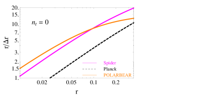
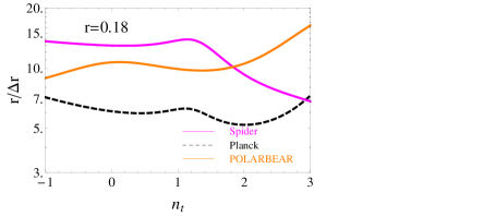
Figure 5: Predicted signal-to-noise of measurements of $r$ for varying $r$ (left panel) and $n_{\rm t}$ (right panel).

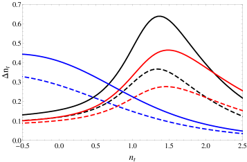
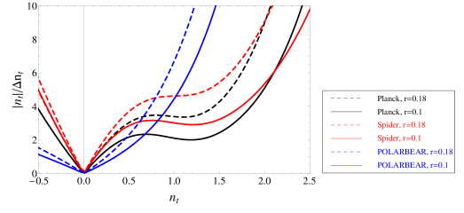
Figure 6: Predicted $\Delta n_{\rm t}$ (left panel) and signal-to-noise $|n_{\rm t}|/\Delta n_{\rm t}$ (right panel) for varying $n_{\rm t}$, with $r=0.18$ and $r=0.1$.

Forecast for future experiments– The tensor-to-scalar ratio is claimed to be $0.18$ at $k_{0}=0.01\,{\rm Mpc}^{-1}$ by BICEP2 experiment BICEP2 . It now is required to determine if $n_{\rm t}$ varies, how precisely can future experiments measure the B-mode polarization.

In Figure 2, we plot the theoretical prediction of $C_{\ell}^{\rm BB}$ with three $n_{\rm t}$ values, using three different noise levels. The first corresponds to that of a Planck-like experiment having the idealised noise performance described in Ref. Planckblue , and the second and third to the Spider and POLARBEAR experiments. We note that for the Planck-like experiment, we have not attempted to model the real performance of Planck, or the effects of systematics, and so every time ’Planck’ is mentioned below in the context of forecasted results, this refers to results from an idealised Planck-like experiment only.

We choose the three representative values of $n_{\rm t}$: (1) $n_{\rm t}=0$, flat tensor spectrum (red solid line); (2) $n_{\rm t}=-r/8$, the $n_{\rm t}$ value that satisfies the consistency relation for single-field slow-roll inflation model Liddle93 (green solid line); (3) $n_{\rm t}=2.6$, the current $3\sigma$ upper limit of Planck+BICEP2 constraint (blue dashed line). We can see that the $n_{\rm t}=-r/8=-0.025$ line does not differ significantly from the flat tensor spectrum. However, as $n_{\rm t}$ becomes more positive, the $C^{\rm BB}_{\ell}$ tends to have more powers on small scales and less power on large scales, due to the blue tilted power spectrum. In addition, we follow the recipes in ref. Ma10 to calculate the noise level of the each experiment. It has been seen that Spider has lower noise than Planck at low-$\ell$, but the effective noise blows up at high $\ell$ because of the large beam. The noise from POLARBAER is systematically lower than Planck and Spider, making it a powerful measurement on primordial tensor mode. We also plot the gravitational lensing signal as the purple dashed line in Figure 2. The gravitational lensing can convert primordial E mode into B mode, therefore add an effective noise to the true primordial B-mode signal. In Figure 2, we can see that this signal peaks at $\ell\approx 1000$ which is the typical galaxy cluster scale. The $C^{\rm len}_{\ell}$ is fixed with a certain set of cosmological parameters and therefore can be outputted from camb cambcode .

In Figure 3, we plot the added signal of primordial tensor mode with gravitational lensing, and the current measurement from BICEP2 BICEP2 and POLARBAER PolarBear . We can see that current data is consistent with the tensor mode with amplitude $r=0.18$, while it still allows a fairly large range of spectral index $n_{\rm t}$.

Assuming each $\ell$ is independent, uncertainties of each $\ell$ of B-mode polarization power spectrum is computed as:

$$\Delta C^{\rm BB}_{\ell}=\sqrt{\frac{2}{(2\ell+1)f_{\rm sky}}}\left(C_{\ell}^{\rm BB}+N_{\ell}^{\rm BB}\right),$$ (4)

where $N_{\ell}$ is the effective noise of each experiment, which includes the instrumental noise, residual foreground contamination, and the gravitational lensing. The value of $f_{\rm sky}$ is the effective area of sky that each experiment observes, which are $0.65$, $0.5$, $0.024$ for Planck Planckblue , Spider Crill08 and POLARBEAR PolarBear , respectively.

In Figure 4, we plot the signal-to-noise of each $\ell$ for the three experiments. We can see that for each experiment, as the $n_{\rm t}$ value becomes more positive, one gains less signal to noise from large scales, but more from small scales. The Spider experiment, because of the large beam, cannot obtain consistent result on large $\ell$s, but its measurement on low-$\ell$ is better than that of Planck. The future POLARBEAR experiment is better than both Spider and Planck. We list the contribution to total signal to noise from $\ell\leq 100$ and $\ell>100$ in Table 1.

Let us forecast for the constraints achievable with future experiments. With the assumption that each parameter is Gaussian-distributed, we calculate the Fisher matrix $F_{\alpha\beta}$ Tegmark97a ; Tegmark97b such that

$$F_{\alpha\beta}=\frac{1}{2}\textrm{Tr}[\mathbf{C}_{,\alpha}\mathbf{C}^{-1}\mathbf{C}_{,\beta}\mathbf{C}^{-1}],$$ (5)

where $\mathbf{C}$ is the total covariance matrix, which includes both signal and noise contributions. In case of B-mode only, where each $\ell$ and $m$ mode is independent of each other, then

$$\mathbf{C}_{\ell_{1}m_{1}\ell_{2}m_{2}}=(C_{\ell_{1}}^{\rm BB}+N_{\ell_{1}}^{\rm BB})\delta_{\ell_{1}\ell_{2}}\delta_{m_{1}m_{2}}.$$ (6)

In this case, the Fisher matrix can be simplified Tegmark97a ; Tegmark97b as:

$$F_{\alpha\beta}=\sum^{\ell_{\rm max}}_{\ell=\ell_{\rm min}}\left(\frac{2\ell+1}{2}f_{\rm sky}\right)\frac{(C_{\ell}^{\rm BB})_{,\alpha}(C_{\ell}^{\rm BB})_{,\beta}}{(C_{\ell}^{\rm BB}+N_{\ell}^{\rm BB})^{2}}.$$ (7)

For Planck and Spider experiment, since the observation is nearly full sky, we perform the summation in eq. (7) to be $\ell_{\rm min}=2$ till $\ell_{\rm max}=3000$. For the ground-based POLARBEAR, the summation is performed from $\ell_{\rm min}=21$ to $\ell_{\rm max}=3000$, since POLARBEAR cannot cover the largest angular scales because of the corresponding finite survey areas.

The inverse of the Fisher matrix $F^{-1}$ can be regarded as the best achievable covariance matrix for the parameters given the experimental specification. The Cramer-Rao inequality suggests that no unbiased method can measure the $i$th parameter with an uncertainty less than $1/\sqrt{F_{ii}}$ Tegmark97a . If the other parameters are not known and considered as free parameters, the minimum standard deviation is $(F^{-1})^{1/2}_{ii}$ Tegmark97a . Therefore the best prospective signal-to-noise ratio can be estimated as $\alpha/\Delta\alpha$, where $\Delta\alpha=(F^{-1})_{\alpha\alpha}^{{1}/{2}}$.

In the left panel of Figure 5, we plot the $r/\Delta r$ as a function of true value of $r$. We can see that the higher the value of $r$ is, the more signal to noise one can obtain from each experiment. The POLARBEAR and Spider experiments provide stronger constraints on $r$ than Planck. In the right panel of Figure 5, we vary the value of $n_{\rm t}$ and calculate the $r/\Delta r$ for each assumed value of $n_{\rm t}$. It can be seen that the for Planck, the measured signal to noise of $r$ is not exceedingly sensitive to the true value of $n_{\rm t}$. But for Spider, as the $n_{\rm t}$ value becomes bigger, the signal to noise decreases because Spider is incapable of measuring high-$\ell$ power accurately. For POLARBEAR, the signal to noise of $r$ is all high across all values of $n_{\rm t}$.

In Figure 6, we plot the noise $\Delta n_{\rm t}$ and the signal-to-noise ratio $n_{\rm t}/\Delta n_{\rm t}$ respectively, for varying $n_{\rm t}$. In the left panel of Figure 6, $\Delta n_{\rm t}$ is about $0.1$ near $n_{\rm t}=0$. Thus it is still challenging for the upcoming experiments to measure the inflationary consistency relation (if $n_{\rm t}=-r/8$). In the right panel of Figure 6, It can be seen that assuming $r\geq 0.1$ and $n_{\rm t}\sim 1$, Planck and Spider are able to confirm the hint for positive $n_{\rm t}$ and POLARBEAR will be sufficiently precise to make a detection.

In Figure 1, we put together the current joint constraints with the forecasted signal-to-noise measurement of parameters $r$-$n_{\rm t}$. The green region is the excluded by current POLARBEAR experiment at $3\sigma$ CL, while the blue and purple contours are the BICEP2 only and Planck+WMAP Polarization(WP)+BICEP2 data. It can be seen that the joint constraint favors a positive range of $n_{\rm t}$ values. We also plot the $r/\Delta r=5$ and $3$ lines in the same figure for Planck, POLARBEAR and Spider experiments. Comparing Planck forecasted lines with the current constraints, one can see only if $r<0.1$ and $2<n_{\rm t}<3$ Planck may not be able to constrain $r$ at $3\sigma$ CL. In all other parameter ranges, Planck can constrain the value better than $3\sigma$ CL. Specifically, if $r>0.15$, Planck should be able to measure it in more than $5\sigma$ CL. Spider and POLARBEAR can do much better than Planck since they can measure nearly the whole parameter space with $r>0.05$ in more $5\sigma$ CL. In addition, as we can see from Figure 1, there is a possibility for future experiments to test the inflationary consistency relation as shown in dashed (nearly vertical) line. But current Planck+BICEP2+WP data favors a large positive value, which does not cover this line at $2\sigma$ CL. Therefore, future experiments will set up a rigorous test on this consistency relation.

Conclusions– The B-mode polarization power spectrum is a unique probe of the primordial tensor fluctuations. Current observations BICEP2 claim that the tensor-to-scalar ratio $r$ is $0.18$ at $0.01\,{\rm Mpc}^{-1}$. If BICEP2 data is correct, $n_{\rm t}$ is constrained to be $n_{\rm t}=1.24\pm 0.90$ ($1\sigma\,$CL) for BICEP2 only, indicating a blue tensor spectrum. By combining the BICEP2 data with Planck data and WMAP polarization data, we find $n_{\rm t}=1.76\pm 0.54$ ($1\sigma\,$CL).

Assuming the true value of $r$ is large and detectable, we forecast the detectability of the parameters $r$ and $n_{\rm t}$ for a Planck-like experiment with the same noise as projected in Ref. (Planckblue, ), and for balloon-borne Spider data and ground-base POLARBEAR data with the current understanding the foreground emission and their experimental noise. We used the Fisher matrix to calculate the forecasted signal-to-noise ratio. We found that if $r>0.1$ and $2<n_{\rm t}<3$, Planck can measure $r$ in more than $3\sigma$ confidence level. POLARBEAR and Spider data are even more powerful than Planck, since they can measure nearly the whole parameter space $r>0.05$ by more than $5\sigma$ CL. The detectability of tensor-to-scalar ratio $r$ for Planck, Spider and POLARBEAR is relatively independent on the details value of $n_{\rm t}$ since the $r/\Delta r=3$ and $5$ lines in Figure 1 are nearly horizontal. However, we caution the reader that if the BICEP2 result is found to be largely due to uncleaned polarized foreground, the true value of $r$ could be significant less than $0.2$. In this case, the signal-to-noise lines of $r$ in Figure. 1 will be very low and might be undetectable. In addition, in our study, we do not consider the running of spectral index (${\rm d}n_{\rm t}/{\rm d}\ln k$) for tensor power spectrum, which in principle, can be nonzero if the spectral index is large. In addition, successful delensing can significantly boost the signal-to-noise ratio, particularly when $n_{\rm t}$ is positive Seljak04 , which is beyond the scope of this paper.

Acknowledgments– We thank BAUMANN D.  and ZHAO W.  for helpful discussions. This work was supported by a CITA National Fellowship, a Starting Grant of the European Research Council (ERC STG Grant No. 279617) and the Stephen Hawking Advanced Fellowship. Part of this work was undertaken on the COSMOS Shared Memory system at DAMTP, University of Cambridge operated on behalf of the STFC DiRAC HPC Facility. This equipment was funded by BIS National E-infrastructure capital grant ST/J005673/1 and STFC grants ST/H008586/1, ST/K00333X/1.

References

- (1) BICEP2 Collaboration. BICEP2 I: Detection Of B-mode polarization at degree angular scales. arXiv:1403.3985 [astro-ph.CO]
- (2) FLAUGER R, COLIN HILL J, SPERGEL D N, Toward an Understanding of Foreground Emission in the BICEP2 Region, arXiv: 1405.7351
- (3) Ma Y Z, Wang Y. Reconstructing the local potential of inflation with BICEP2 data. arXiv:1403.4585 [astro-ph.CO]
- (4) Xia J Q, Cai Y F, Li H, et al. Evidence for bouncing evolution before inflation after BICEP2. arXiv:1403.7623 [astro-ph.CO]
- (5) Cai Y F, Quintin J, Saridakis E N, et al. Nonsingular bouncing cosmologies in light of BICEP2. arXiv:1404.4364 [astro-ph.CO]
- (6) Cai Y F. Exploring bouncing cosmologies with cosmological surveys. Sci China-Phys Mech Astron, 2014, 57(8): 1111-1112
- (7) Gerbino M, Marchini A, Pagano L, et al. Blue gravity waves from BICEP2? arXiv:1403.5732 [astro-ph.CO]
- (8) Wang Y, Xue W. Inflation and alternatives with blue tensor spectra. arXiv:1403.5817 [astro-ph.CO]
- (9) Ashoorioon A, Dimopoulos K, Sheikh-Jabbari M M, et al. Non-bunch-Davis initial state reconciles chaotic models with BICEP and Planck. arXiv:1403.6099 [hep-th]
- (10) Smith K M, Dvorkin C, Boyle L, et al. On quantifying and resolving the BICEP2/Planck tension over gravitational waves. arXiv:1404.0373 [astro-ph.CO]
- (11) Planck Collaboration. Planck 2013 results. XV. CMB power spectra and likelihood arXiv:1303.5075 [astro-ph.CO]
- (12) Liu Z -G, Li H, Piao Y -S, Pre-inflationary genesis with CMB B-mode polarization. arXiv:1405.1188 [astro-ph.CO].
- (13) Cai Y F, Wang Y. Testing quantum gravity effects with latest CMB observations. arXiv:1404.6672 [astro-ph.CO]
- (14) Wu F, Li Y, Lu Y, et al. Cosmological parameter fittings with the BICEP2 data. arXiv:1403.6462 [astro-ph.CO]
- (15) Li H, Xia J Q, Zhang X M. Global fitting analysis on cosmological models after BICEP2. arXiv:1404.0238 [astro-ph.CO]
- (16) Crill B P, Ade P A R, Battistelli E S, et al. SPIDER: A balloon-borne large-scale CMB polarimeter. SPIE, 2008, 7010: 79
- (17) POLARBEAR Collaboration. A measurement of the cosmic microwave background B-mode polarization power spectrum at sub-degree scales with POLARBEAR. arXiv: 1403.2369 [astro-ph.CO]
- (18) Lewis A, Challinor A, Lasenby A. Efficient computation of cosmic microwave background anisotropies in closed Friedmann-Robertson-Walker models. Astrophys J, 2000, 538: 473–476, http://www.camb.info
- (19) Lewis A, Bridle S. Cosmological parameters from CMB and other data: A Monte Carlo approach. Phys Rev D, 2002, 66: 103511
- (20) Liddle A R, Lyth D H. The cold dark matter density perturbation. Phys Rept, 1993, 231: 1–105
- (21) Ma Y Z, Zhao W, Brown M L. Testing early Universe models from B-mode polarization. J Cosmol Astropart Phys, 2010, 10: 007
- (22) Planck Collaboration. Planck: The scientific programme. European Space Agency Vol. No. ESA–SCI (2005)1. In: Efstathiou G, ed. Netherlands: ESA Publications, Noordwijk, 2005
- (23) Tegmark M, Taylor A, Heavens A. Karhunen-Loeve eigenvalue problems in cosmology: How should we tackle large data sets? Astrophys J, 1997, 480: 22–35
- (24) Tegmark M. Measuring cosmological parameters with galaxy surveys. Phys Rev Lett, 1997, 79: 3806–3809
- (25) Seljak U, Hirata C M. Gravitational lensing as a contaminant of the gravity wave signal in CMB. Phys Rev D, 2004, 69: 043005