Learning the Information Divergence

Abstract

Information divergence that measures the difference between two nonnegative matrices or tensors has found its use in a variety of machine learning problems. Examples are Nonnegative Matrix/Tensor Factorization, Stochastic Neighbor Embedding, topic models, and Bayesian network optimization. The success of such a learning task depends heavily on a suitable divergence. A large variety of divergences have been suggested and analyzed, but very few results are available for an objective choice of the optimal divergence for a given task. Here we present a framework that facilitates automatic selection of the best divergence among a given family, based on standard maximum likelihood estimation. We first propose an approximated Tweedie distribution for the $\beta$-divergence family. Selecting the best $\beta$ then becomes a machine learning problem solved by maximum likelihood. Next, we reformulate $\alpha$-divergence in terms of $\beta$-divergence, which enables automatic selection of $\alpha$ by maximum likelihood with reuse of the learning principle for $\beta$-divergence. Furthermore, we show the connections between $\gamma$- and $\beta$-divergences as well as Rényi- and $\alpha$-divergences, such that our automatic selection framework is extended to non-separable divergences. Experiments on both synthetic and real-world data demonstrate that our method can quite accurately select information divergence across different learning problems and various divergence families.

I Introduction

Information divergences are an essential element in modern machine learning. They originated in estimation theory where a divergence maps the dissimilarity between two probability distributions to nonnegative values. Presently, information divergences have been extended for nonnegative tensors and used in many learning problems where the objective is to minimize the approximation error between the observed data and the model. Typical applications include Nonnegative Matrix Factorization (see e.g. [1, 2, 3, 4]), Stochastic Neighbor Embedding [5, 6], topic models [7, 8], and Bayesian network optimization [9].

There exist a large variety of information divergences. In Section II, we summarize the most popularly used parametric families including $\alpha$-, $\beta$-, $\gamma$- and Rényi-divergences [10, 11, 12, 13, 14] and their combinations (e.g. [15]). The four parametric families in turn belong to broader ones such as the Csiszár-Morimoto $f$-divergences [16, 17] and Bregman divergences [18]. Data analysis techniques based on information divergences have been widely and successfully applied to various data such as text [19], electroencephalography [3], facial images [20], and audio spectrograms [21].

Compared to the rich set of available information divergences, there is little research on how to select the best one for a given application. This is an important issue because the performance of a given divergence-based estimation or modeling method in a particular task very much depends on the divergence used. Formulating a learning task in a family of divergences greatly increases the flexibility to handle different types of noise in data. For example, Euclidean distance is suitable for data with Gaussian noise; Kullback-Leibler divergence has shown success for finding topics in text documents [7]; and Itakura-Saito divergence has proven to be suitable for audio signal processing [21]. A conventional workaround is to select among a finite number of candidate divergences using a validation set. This however cannot be applied to divergences that are non-separable over tensor entries. The validation approach is also problematic for tasks where all data are needed for learning, for example, cluster analysis.

In Section III, we propose a new method of statistical learning for selecting the best divergence among the four popular parametric families in any given data modeling task. Our starting-point is the Tweedie distribution [22], which is known to have a relationship with $\beta$-divergence [23, 24]. The Maximum Tweedie Likelihood (MTL) is in principle a disciplined and straightforward method for choosing the optimal $\beta$ value. However, in order for this to be feasible in practice, two shortcomings with the MTL method have to be overcome: 1) Tweedie distribution is not defined for all $\beta$; 2) calculation of Tweedie likelihood is complicated and prone to numerical problems for large $\beta$. To overcome these drawbacks, we propose here a novel distribution using an exponential over the $\beta$-divergence with a specific augmentation term. The new distribution has the following nice properties: 1) it is close to the Tweedie distribution, especially at four important special cases; 2) it exists for all $\beta\in\mathbb{R}$; 3) its likelihood can be calculated by standard statistical software. We call the new density the Exponential Divergence with Augmentation (EDA). EDA is a non-normalized density, i.e., its likelihood includes a normalizing constant which is not analytically available. But, since the density is univariate the normalizing constant can be efficiently and accurately estimated by numerical integration. The method of Maximizing the Exponential Divergence with Augmentation Likelihood (MEDAL) thus gives a more robust $\beta$ selection in a wider range than MTL. $\beta$ estimation on EDA can also be carried out using parameter estimation methods, e.g., Score Matching (SM) [25], specifically proposed for non-normalized densities. In the experiments section, we show that SM on EDA also performs as accurately as MEDAL.

Besides $\beta$-divergence, the MEDAL method is extended to select the best divergence in other parametric families. We reformulate $\alpha$-divergence in terms of $\beta$-divergence after a change of parameters so that $\alpha$ can be optimized using the MEDAL method. Our method can also be applied to non-separable cases. We show the equivalence between $\beta$ and $\gamma$-divergences, and between $\alpha$ and Rényi divergences by a connecting scalar, which allows us to choose the best $\gamma$- or Rényi-divergence by reusing the MEDAL method.

We tested our method with extensive experiments, whose results are presented in Section IV. We have used both synthetic data with a known distribution and real-world data including music, stock prices, and social networks. The MEDAL method is applied to different learning problems: Nonnegative Matrix Factorization (NMF) [26, 3, 1], Projective NMF [27, 28] and Symmetric Stochastic Neighbor Embedding for visualization [5, 6]. We also demonstrate that our method outperforms Score Matching on Exponential Divergence distribution (ED), a previous approach for $\beta$-divergence selection [29]. Conclusions and discussions on future work are given in Section V.

II Information Divergences

Many learning objectives can be formulated as an approximation of the form $\mathbf{x}\approx\bm{\mu}$, where $\mathbf{x}>0$ is the observed data (input) and $\bm{\mu}$ is the approximation given by the model. The formulation for $\bm{\mu}$ totally depends on the task to be solved. Consider Nonnegative Matrix Factorization: then $\mathbf{x}>0$ is a data matrix and $\bm{\mu}$ is a product of two lower-rank nonnegative matrices which typically give a sparse representation for the columns of $\mathbf{x}$. Other concrete examples are given in Section IV.

The approximation error can be measured by various information divergences. Suppose $\bm{\mu}$ is parameterized by $\bm{\Theta}$. The learning problem becomes an optimization procedure that minimizes the given divergence $D(\mathbf{x}||\bm{\mu}(\bm{\Theta}))$ over $\bm{\Theta}$. Regularization may be applied for $\bm{\Theta}$ for complexity control. For notational brevity we focus on definitions over vectorial $\mathbf{x}$, $\bm{\mu}$, $\bm{\Theta}$ in this section, while they can be extended to matrices or higher order tensors in a straightforward manner.

In this work we consider four parametric families of divergences, which are the widely used $\alpha$-, $\beta$-, $\gamma$- and Rényi-divergences. This collection is rich because it covers most commonly used divergences. The definition of the four families and some of their special cases are given below.

• $\alpha$-divergence [10, 11] is defined as

  $$D_{\alpha}(\mathbf{x}||\bm{\mu})=\frac{\sum_{i}x_{i}^{\alpha}\mu_{i}^{1-\alpha}-\alpha x_{i}+(\alpha-1)\mu_{i}}{\alpha(\alpha-1)}.$$ (1)

  The family contains the following special cases:

  $$D_{\alpha=2}(\mathbf{x}||\bm{\mu})= D_{\text{P}}(\mathbf{x}||\bm{\mu})=\frac{1}{2}\sum_{i}\frac{(x_{i}-\mu_{i})^{2}}{\mu_{i}}$$

  $$D_{\alpha\rightarrow 1}(\mathbf{x}||\bm{\mu})= D_{\text{I}}(\mathbf{x}||\bm{\mu})=\sum_{i}\left(x_{i}\ln\frac{x_{i}}{\mu_{i}}-x_{i}+\mu_{i}\right)$$

  $$D_{\alpha=1/2}(\mathbf{x}||\bm{\mu})= 2D_{\text{H}}(\mathbf{x}||\bm{\mu})=2\sum_{i}(\sqrt{x_{i}}-\sqrt{\mu_{i}})^{2}$$

  $$D_{\alpha\rightarrow 0}(\mathbf{x}||\bm{\mu})= D_{\text{I}}(\bm{\mu}||\mathbf{x})=\sum_{i}\left(\mu_{i}\ln\frac{\mu_{i}}{x_{i}}-\mu_{i}+x_{i}\right)$$

  $$D_{\alpha=-1}(\mathbf{x}||\bm{\mu})= D_{\text{IP}}(\mathbf{x}||\bm{\mu})=\frac{1}{2}\sum_{i}\frac{(x_{i}-\mu_{i})^{2}}{x_{i}}$$

  where $D_{\text{I}}$, $D_{\text{P}}$, $D_{\text{IP}}$, and $D_{\text{H}}$ denote non-normalized Kullback-Leibler, Pearson Chi-square, inverse Pearson and Hellinger distances, respectively.

• $\beta$-divergence [30, 31] is defined as

  $$D_{\beta}(\mathbf{x}||\bm{\mu})=\frac{\sum_{i}x_{i}^{\beta+1}+\beta\mu_{i}^{\beta+1}-(\beta+1)x_{i}\mu_{i}^{\beta}}{\beta(\beta+1)}.$$ (2)

  The family contains the following special cases:

  $$D_{\beta=1}(\mathbf{x}||\bm{\mu})= D_{\text{EU}}(\mathbf{x}||\bm{\mu})=\frac{1}{2}\sum_{i}(x_{i}-\mu_{i})^{2}$$ (3)

  $$D_{\beta\rightarrow 0}(\mathbf{x}||\bm{\mu})= D_{\text{I}}(\mathbf{x}||\bm{\mu})=\sum_{i}\left(x_{i}\ln\frac{x_{i}}{\mu_{i}}-x_{i}+\mu_{i}\right)$$ (4)

  $$D_{\beta\rightarrow-1}(\mathbf{x}||\bm{\mu})= D_{\text{IS}}(\mathbf{x}||\bm{\mu})=\sum_{i}\left(\frac{x_{i}}{\mu_{i}}-\ln\frac{x_{i}}{\mu_{i}}-1\right)$$ (5)

  $$D_{\beta=-2}(\mathbf{x}||\bm{\mu})= \sum_{i}\left(\frac{x_{i}}{2\mu_{i}^{2}}-\frac{1}{\mu_{i}}+\frac{1}{2x_{i}}\right),$$ (6)

  where $D_{\mathrm{EU}}$ and $D_{\mathrm{IS}}$ denote the Euclidean distance and Itakura-Saito divergence, respectively.

• $\gamma$-divergence [13] is defined as

  $$D_{\gamma}(\mathbf{x}||\bm{\mu})= \frac{1}{\gamma(\gamma+1)}\left[\ln\left(\sum_{i}x_{i}^{\gamma+1}\right)+\gamma\ln\left(\sum_{i}\mu_{i}^{\gamma+1}\right)\right.$$

  $$\left.-(\gamma+1)\ln\left(\sum_{i}x_{i}\mu_{i}^{\gamma}\right)\right].$$ (7)

  The normalized Kullback-Leibler (KL) divergence is a special case of $\gamma$-divergence:

  $$D_{\gamma\rightarrow 0}(\mathbf{x}||\bm{\mu})=D_{\mathrm{KL}}(\tilde{\mathbf{x}}||\tilde{\bm{\mu}})=\sum_{i}\tilde{x}_{i}\ln\frac{\tilde{x}_{i}}{\tilde{\mu}_{i}},$$ (8)

  where $\tilde{x}_{i}=x_{i}/\sum_{j}x_{j}$ and $\tilde{\mu}_{i}=\mu_{i}/\sum_{j}\mu_{j}$.

• Rényi divergence [32] is defined as

  $$D_{\rho}(\mathbf{x}||\bm{\mu})=\frac{1}{\rho-1}\ln\left(\tilde{x}_{i}^{\rho}\tilde{\mu}_{i}^{1-\rho}\right)$$ (9)

  for $\rho>0$. The Rényi divergence also includes the normalized Kullback-Leibler divergence as its special case when $\rho\rightarrow 1$.

III Divergence Selection by Statistical Learning

The above rich collection of information divergences basically allows great flexibility to the approximation framework. However, practitioners must face a choice problem: how to select the best divergence in a family? In most existing applications the selection is done empirically by the human. A conventional automatic selection method is cross-validation [33, 34], where the training only uses part of the entries of $\mathbf{x}$ and the remaining ones are used for validation. This method has a number of drawbacks: 1) it is only applicable to the divergences where the entries are separable (e.g. $\alpha$- or $\beta$-divergence). Leaving out some entries for $\gamma$- and Rényi divergences is infeasible due to the logarithm or normalization; 2) separation of entries is not applicable in some applications where all entries are needed in the learning, for example, cluster analysis.

Our proposal here is to use the familiar and proven technique of maximum likelihood estimation for automatic divergence selection, using a suitably chosen and very flexible probability density model for the data. In the following we discuss this statistical learning approach for automatic divergence selection in the family of $\beta$ -divergences, followed by its extensions to the other divergence families.

III-A Selecting $\beta$-divergence

III-A1 Maximum Tweedie Likelihood (MTL)

We start from the probability density function (pdf) of an exponential dispersion model (EDM) [22]:

$$p_{\text{EDM}}(x;\theta,\phi,p)=f(x,\phi,p)\exp\left[\frac{1}{\phi}(x\theta-\kappa(\theta))\right]$$ (10)

where $\phi>0$ is the dispersion parameter, $\theta$ is the canonical parameter, and $\kappa(\theta)$ is the cumulant function (when $\phi=1$ its derivatives w.r.t. $\theta$ give the cumulants). Such a distribution has mean $\mu=\kappa^{\prime}(\theta)$ and variance $V(\mu,p)=\phi\kappa^{\prime\prime}(\theta)$. This density is defined for $x\geq 0$, thus $\mu>0$.

A Tweedie distribution is an EDM whose variance has a special form, $V(\mu)=\mu^{p}$ with $p\in\mathbb{R}\backslash(0,1)$. The canonical parameter and the cumulant function that satisfy this property are [22]

$$\theta=\left\{\begin{array}[]{rl}\frac{\mu^{1-p}-1}{1-p},&\mbox{ if $p\neq 1$}\\ \ln\mu,&\mbox{ if $p=1$}\end{array}\right.,\;\;\;\;\kappa(\theta)=\left\{\begin{array}[]{rl}\frac{\mu^{2-p}-1}{2-p},&\mbox{ if $p\neq 2$}\\ \ln\mu,&\mbox{ if $p=2$}\end{array}\right.\;.$$ (15)

Note that $\ln\mu$ is the limit of $\frac{\mu^{t}-1}{t}$ as $t\to 0$. Finite analytical forms of $f(x,\phi,p)$ in Tweedie distribution are generally unavailable. The function can be expanded with infinite series [35] or approximated by saddle point estimation [36].

It is known that the Tweedie distribution has a connection to $\beta$-divergence (see, e.g., [23, 24]): maximizing the likelihood of Tweedie distribution for certain $p$ values is equivalent to minimizing the corresponding divergence with $\beta=1-p$. Especially, the gradients of the log-likelihood of Gamma, Poisson and Gaussian distributions over $\mu_{i}$ are equal to the ones of $\beta$-divergence with $\beta=-1,0,1$, respectively. This motivates a $\beta$-divergence selection method by Maximum Tweedie Likelihood (MTL).

However, MTL has the following two shortcomings. First, Tweedie distribution is not defined for $p\in(0,1)$. That is, if the best $\beta=1-p$ happens to be in the range $(0,1)$, it cannot be found by MTL; in addition, there is little research on the Tweedie distribution with $\beta>1\;(p<0)$. Second, $f(x,\phi,p)$ in Tweedie distribution is not the probability normalizing constant (note that it depends on $x$), and its evaluation requires ad hoc techniques. The existing software using the infinite series expansion approach [35] (see Appendix A) is prone to numerical computation problems especially for $-0.1<\beta<0$. There is no existing implementation that can calculate Tweedie likelihood for $\beta>1$.

III-A2 Maximum Exponential Divergence with Augmentation Likelihood (MEDAL)

Our answer to the above shortcomings in MTL is to design an alternative distribution with the following properties: 1) it is close to the Tweedie distribution, especially for the four crucial points when $\beta\in\{-2,-1,0,1\}$; 2) it should be defined for all $\beta\in\mathbb{R}$; 3) its pdf can be evaluated more robustly by standard statistical software.

From (10) and (15) the pdf of the Tweedie distribution is written as

$$p_{\text{Tw}}(x;\mu,\phi,\beta) =f(x,\phi,\beta)\exp\left[\frac{1}{\phi}\left(\frac{x\mu^{\beta}}{\beta}-\frac{\mu^{\beta+1}}{{\beta+1}}\right)\right]$$ (16)

w.r.t. $\beta$ instead of $p$, using the relation $\beta=1-p$. This holds when $\beta\neq 0$ and $\beta\neq-1$. The extra terms $1/(1-p)$ and $1/(2-p)$ in (15) have been absorbed in $f(x,\phi,\beta)$. The cases $\beta=0$ or $\beta=-1$ have to be analyzed separately.

To make an explicit connection with $\beta$-divergence defined in (2), we suggest a new distribution given in the following form:

$$p_{\text{approx}}(x;\mu,\phi,\beta)=g(x,\phi,\beta)\exp\left\{-\frac{1}{\phi}D_{\beta}(x||\mu)\right\}$$

$$=g(x,\phi,\beta)\exp\left[\frac{1}{\phi}\left(-\frac{x^{\beta+1}}{\beta({\beta+1})}+\frac{x\mu^{\beta}}{\beta}-\frac{\mu^{\beta+1}}{{\beta+1}}\right)\right].$$ (17)

Now the $\beta$-divergence for scalar $x$ appears in the exponent, and $g(x,\phi,\beta)$ will be used to approximate this with the Tweedie distribution. Ideally, the choice

$$g(x,\phi,\beta)=f(x,\phi,\beta)/\exp\left[\frac{1}{\phi}\left(-\frac{x^{\beta+1}}{\beta({\beta+1})}\right)\right]$$

would result in full equivalence to Tweedie distribution, as seen from (16). However, because $f(x,\phi,\beta)$ is unknown in the general case, such $g$ is also unavailable.

We can, however, try to approximate $g$ using the fact that $p_{\text{approx}}$ must be a proper density whose integral is equal to one. From (17) it then follows

$$\exp\left[\frac{1}{\phi}\frac{\mu^{\beta+1}}{{\beta+1}}\right]$$

$$=\int dx\,g(x,\phi,\beta)\exp\left[\frac{1}{\phi}\left(-\frac{x^{\beta+1}}{\beta({\beta+1})}+\frac{x\mu^{\beta}}{\beta}\right)\right]$$ (18)

This integral is, of course, impossible to evaluate because we do not even know the function inside. However, the integral can be approximated nicely by Laplace’s method. Laplace’s approximation is

$$\int_{a}^{b}dx\,f(x)e^{Mh(x)}\approx\sqrt{\frac{2\pi}{M|h^{\prime\prime}(x_{0})|}}f(x_{0})e^{Mh(x_{0})}$$

where $x_{0}=\arg\max_{x}h(x)$ and $M$ is a large constant.

In order to approximate (18) by Laplace’s method, $1/\phi$ takes the role of $M$ and thus the approximation is valid for small $\phi$. We need the maximizer of the exponentiated term $h(x)=-\frac{x^{\beta+1}}{\beta({\beta+1})}+\frac{x\mu^{\beta}}{\beta}$. This term has a zero first derivative and negative second derivative, i.e., it is maximized, at $x=\mu$. Thus, Laplace’s method gives us

$$\exp\left[\frac{1}{\phi}\frac{\mu^{\beta+1}}{{\beta+1}}\right]$$

$$\approx\sqrt{\frac{2\pi\phi}{|-\mu^{\beta-1}|}}\;g(\mu,\phi,\beta)\exp\left[\frac{1}{\phi}\left(-\frac{\mu^{\beta+1}}{\beta({\beta+1})}+\frac{\mu^{\beta+1}}{\beta}\right)\right]$$

$$=\sqrt{\frac{2\pi\phi}{\mu^{\beta-1}}}\;g(\mu,\phi,\beta)\exp\left[\frac{1}{\phi}\frac{\mu^{\beta+1}}{{\beta+1}}\right]\,.$$

The approximation gives $g(\mu,\phi,\beta)=\frac{1}{\sqrt{2\pi\phi}}\mu^{({\beta-1})/2}$ which suggests the function

$$g(x,\phi,\beta)=\frac{1}{\sqrt{2\pi\phi}}x^{({\beta-1})/2}\,=\frac{1}{\sqrt{2\pi\phi}}\exp\left[\frac{({\beta-1})}{2}\ln x\right].$$

Putting this result into (17) as such does not guarantee a proper pdf however, because it is an approximation, only valid at the limit $\phi\to 0$. To make it proper, we have to add a normalizing constant into the density in (17).

The pdf of the final distribution, for a scalar argument $x$, thus becomes

$$p_{\text{approx}}(x;\mu,\beta,\phi)=\frac{1}{Z(\mu,\beta,\phi)}\exp\left\{R(x,\beta)-\frac{1}{\phi}D_{\beta}(x||\mu)\right\}$$ (19)

where $Z(\mu,\beta,\phi)$ is the normalizing constant counting for the terms which are independent of $x$, and $R(x,\beta)$ is an augmentation term given as

$$R(x,\beta)=\frac{\beta-1}{2}\ln x\,.$$ (20)

This pdf is a proper density for all $\beta\in\mathbb{R}$, which is guaranteed by the following theorem.

Theorem 1

Let $f(x)=\exp\left\{\frac{\beta-1}{2}\ln x-\frac{1}{\phi}D_{\beta}(x||\mu)\right\}$. The improper integral $\int_{0}^{\infty}f(x)dx$ converges.

Proof:

Let $q=\left|\frac{\beta-1}{2}\right|+1+\epsilon$ with any $\epsilon\in(0,\infty)$, and $g(x)=x^{-q}$. By these definitions, we have $q>\left|\frac{\beta-1}{2}\right|$, and then for $x\geq 1$, $\left(\frac{\beta-1}{2}+q\right)\phi\ln x\leq 0\leq D_{\beta}(x||\mu)$, i.e. $0\leq f(x)\leq g(x)$. By Cauchy convergence test, we know that $\int_{1}^{\infty}g(x)dx$ is convergent because $q>1$, and so is $\int_{1}^{\infty}f(x)dx$. Obviously $f(x)$ is continuous and bounded for $x\in[0,1]$. Therefore, for $x\geq 0$, $\int_{0}^{\infty}f(x)dx=\int_{0}^{1}f(x)dx+\int_{1}^{\infty}f(x)dx$ also converges. ∎

Finally, for vectorial $\mathbf{x}$, the pdf is a product of the marginal densities:

$$p_{\text{EDA}}(\mathbf{x};\bm{\mu},\beta,\phi)=\frac{1}{Z(\bm{\mu},\beta,\phi)}\exp\left\{R(\mathbf{x},\beta)-\frac{1}{\phi}D_{\beta}(\mathbf{x}||\bm{\mu})\right\}$$ (21)

where $D_{\beta}(\mathbf{x}||\bm{\mu})$ is defined in (2) and

$$R(\mathbf{x},\beta)=\frac{\beta-1}{2}\sum_{i}\ln x_{i}\,.$$ (22)

We call (21) the Exponential Divergence with Augmentation (EDA) distribution, because it applies an exponential over an information divergence plus an augmentation term.

The log-likelihood of the EDA density can be written as

$$\ln p(\mathbf{x};\bm{\mu},\beta,\phi)=\sum_{i}\ln p(x_{i};\mu_{i},\beta,\phi)\\ =\sum_{i}\left[\frac{\beta-1}{2}\ln x_{i}-\frac{1}{\phi}D_{\beta}(x_{i}||\mu_{i})-\ln Z(\mu_{i},\beta,\phi)\right]$$ (23)

due to the fact that $D_{\beta}(\mathbf{x}||\bm{\mu})$ in Eq. (2) and the augmentation term in (22) are separable over $x_{i}$, (i.e. $x_{i}$ are independent given $\mu_{i}$). The best $\beta$ is now selected by

$$\beta^{*}=\arg\max_{\beta}\left[\max_{\phi}\ln p(\mathbf{x};\bm{\mu},\beta,\phi)\right]\,,$$ (24)

where $\bm{\mu}=\arg\min_{\bm{\eta}}~{}D_{\beta}(\mathbf{x}||\bm{\eta})$. We call the new divergence selection method Maximum EDA Likelihood (MEDAL).

Let us look at the four special cases of Tweedie distribution: Gaussian ($\mathcal{N}$), Poisson ($\mathcal{P}\mathcal{O}$), Gamma ($\mathcal{G}$) and Inverse Gaussian ($\mathcal{I}\mathcal{N}$). They correspond to $\beta=1,0,-1,-2$. For simplicity of notation, we may drop the subscript $i$ and write $x$ and $\mu$ for one entry in $\mathbf{x}$ and $\bm{\mu}$. Then, the log-likelihoods of the above four special cases are

$$\ln p_{\mathcal{N}}(x;\mu,\phi)= -\frac{1}{2}\ln(2\pi\phi)-\frac{1}{2\phi}(x-\mu)^{2},$$

$$\ln p_{\mathcal{P}\mathcal{O}}(x;\mu)= x\ln\mu-\mu-\ln\Gamma(x+1),$$

$$\approx x\ln\mu-\mu-\ln(2\pi x)/2-x\ln x+x,$$

$$\ln p_{\mathcal{G}}(x;1/\phi,\phi\mu)= (1/\phi-1)\ln x-\frac{x}{\phi\mu}$$

$$-(1/\phi)\ln(\phi\mu)-\ln\Gamma(1/\phi),$$

$$\ln p_{\mathcal{I}\mathcal{N}}(x;\mu,1/\phi)= -\frac{1}{2}\ln(2\pi\phi x^{3})-\frac{1}{\phi}\left(\frac{1}{2}\frac{x}{\mu^{2}}-\frac{1}{\mu}+\frac{1}{2x}\right),$$

where in the Poisson case we employ Stirling’s approximation. To see the similarity of these four special cases with the general expression for the EDA log-likelihood in Eq. (23), let us look at one term in the sum there. It is a fairly straightforward exercise to plug in the $\beta$-divergences from Eqs. (3,4,5,6) and the augmentation term from Eq. (22) and see that the log-likelihoods coincide. The normalizing term $\ln Z(\mu,\beta,\phi)]$ for these special cases can be determined from the corresponding density.

In general, the normalizing constant $Z(\bm{\mu},\beta,\phi)$ is intractable except for a few special cases. Numerical evaluation of $Z(\bm{\mu},\beta,\phi)$ can be implemented by standard statistical software. Here we employ the approximation with Gauss-Laguerre quadratures (details in Appendix B).

Finally, let us note that in addition to the maximum likelihood estimator, Score Matching (SM) [25, 37] can be applied to estimation of $\beta$ as a density parameter (see Section IV-A). In a previous effort, Lu et al. [29] proposed a similar exponential divergence (ED) distribution

$$p_{\text{ED}}(\mathbf{x};\bm{\mu},\beta)\propto\exp\left[-D_{\beta}(\mathbf{x}||\bm{\mu})\right],$$ (25)

but without the augmentation. It is easy to show that ED also exists for all $\beta$ by changing $q=1+\epsilon$ in the proof of Theorem 1. We will empirically illustrate the discrepancy between ED and EDA in Section IV-A, showing that the selection based on ED is however inaccurate, especially for $\beta\leq 0$.

III-B Selecting $\alpha$-divergence

We extend the MEDAL method to $\alpha$-divergence selection. This is done by relating $\alpha$-divergence to $\beta$-divergence with a nonlinear transformation between $\alpha$ and $\beta$. Let $y_{i}=x_{i}^{\alpha}/\alpha^{2\alpha}$, $m_{i}=\mu_{i}^{\alpha}/\alpha^{2\alpha}$ and $\beta=1/\alpha-1$ for $\alpha\neq 0$. We have

$$D_{\beta}(y_{i}||m_{i})= \frac{1}{\beta(\beta+1)}\left(y_{i}^{\beta+1}+\beta m_{i}^{\beta+1}-(\beta+1)y_{i}m_{i}^{\beta}\right)$$

$$= \frac{-\alpha^{2}}{\alpha-1}\left(\frac{x_{i}}{\alpha^{2}}+\frac{1-\alpha}{\alpha}\frac{\mu_{i}}{\alpha^{2}}-\frac{1}{\alpha}\frac{x_{i}^{\alpha}}{\alpha^{2\alpha}}\frac{\mu_{i}^{1-\alpha}}{\alpha^{2(1-\alpha)}}\right)$$

$$= D_{\alpha}(x_{i}||\mu_{i})$$

This relationship allows us to evaluate the likelihood of $\mu$ and $\alpha$ using $y_{i}$ and $\beta$:

$$p(x_{i};\mu_{i},\alpha,\phi) =p(y_{i};m_{i},\beta,\phi)\left|\frac{dy_{i}}{dx_{i}}\right|$$

$$=p(y_{i};m_{i},\beta,\phi)\frac{x_{i}^{\alpha-1}}{\alpha^{2(\alpha-1/2)}}$$

$$=p(y_{i};m_{i},\beta,\phi)y_{i}^{-\beta}|\beta+1|$$

In vectorial form, the best $\alpha$ for $D_{\alpha}(\mathbf{x}||\bm{\mu})$ is then given by $\alpha^{*}=1/(\beta^{*}+1)$ where

$$\beta^{*}= \arg\max_{\beta}\Big{\{}\max_{\phi}\big{[}\ln p(\mathbf{y};\mathbf{m},\beta)$$

$$-\beta\ln y_{i}+\ln|\beta+1|\big{]}\Big{\}},$$ (26)

where $\mathbf{m}=\arg\min_{\bm{\eta}}D_{\beta}(\mathbf{y}||\bm{\eta})$. This transformation method can handle all $\alpha$ except $\alpha\rightarrow 0$ since it corresponds to $\beta\rightarrow\infty$.

III-C Selecting $\gamma$- and Rényi divergences

Above we presented the selection methods for two families where the divergence is separable over the tensor entries. Next we consider selection among $\gamma$- and Rényi divergence families where their members are not separable. Our strategy is to reduce $\gamma$-divergence to $\beta$-divergence with a connecting scalar. This is formally given by the following result.

Theorem 2

For $\mathbf{x}\geq\mathbf{0}$ and $\tau\in\mathbb{R}$,

$$\arg\min_{\bm{\mu}\geq\mathbf{0}}D_{\gamma\rightarrow\tau}(\mathbf{x}||\bm{\mu})=\arg\min_{\bm{\mu}\geq\mathbf{0}}\left[\min_{c>0}D_{\beta\rightarrow\tau}(\mathbf{x}||c\bm{\mu})\right]$$ (27)

The proof is done by zeroing the derivative right hand side with respect to $c$ (details in Appendix C).

Theorem 2 states that with a positive scalar, the learning problem formulated by a $\gamma$-divergence is equivalent to the one by the corresponding $\beta$-divergence. The latter is separable and can be solved by the methods described in the Section III-A. An example is between normalized KL-divergence (in $\gamma$-divergence) and the non-normalized KL-divergence (in $\beta$-divergence) with the optimal connecting scalar $c=\frac{\sum_{i}x_{i}}{\sum_{i}\mu_{i}}$. Example applications on selecting the best $\gamma$-divergence are given in Section IV-D.

Similarly, we can also reduce a Rényi divergence to its corresponding $\alpha$-divergence with the same proof technique (see Appendix C).

Theorem 3

For $\mathbf{x}\geq\mathbf{0}$ and $\tau>0$,

$$\arg\min_{\bm{\mu}\geq\mathbf{0}}D_{\rho\rightarrow\tau}(\mathbf{x}||\bm{\mu})=\arg\min_{\bm{\mu}\geq\mathbf{0}}\left[\min_{c>0}D_{\alpha\rightarrow\tau}(\mathbf{x}||c\bm{\mu})\right].$$ (28)

IV Experiments

In this section we demonstrate the proposed method on various data types and learning tasks. First we provide the results on synthetic data, whose density is known, to compare the behavior of MTL, MEDAL and the score matching method [29]. Second, we illustrate the advantage of the EDA density over ED. Third, we apply our method on $\alpha$- and $\beta$-divergence selection in Nonnegative Matrix Factorization (NMF) on real-world data including music and stock prices. Fourth, we test MEDAL in selecting non-separable cases (e.g. $\gamma$-divergence) for Projective NMF and s-SNE visualization learning tasks across synthetic data, images, and a dolphin social network.

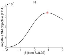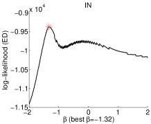
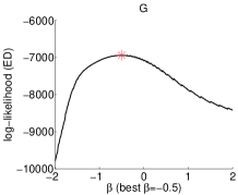
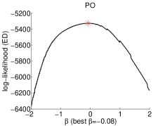
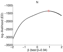
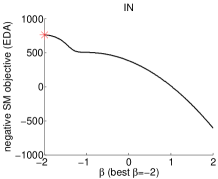
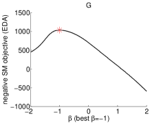
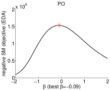
a) Inverse Gaussian	b) Gamma	c) Poisson	d) Gaussian

Figure 1: $\beta$ selection using (from top to bottom) Tweedie likelihood, ED likelihood, negative SM objective of ED, EDA likelihood, and negative SM objective of EDA. Data were generated using Tweedie distribution with $\beta=-2,-1,0,1$ (from left to right).

IV-A Synthetic data

IV-A1 $\beta$-divergence selection

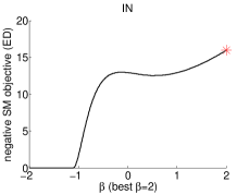
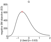
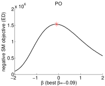
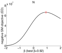
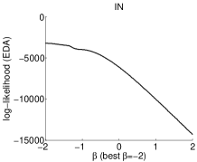
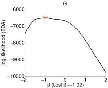
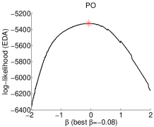
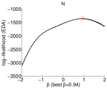
We use here scalar data generated from the four special cases of Tweedie distributions, namely, Inverse Gaussian, Gamma, Poisson, and Gaussian distributions. We simply fit the best Tweedie, EDA or ED density to the data using either the maximum likelihood method or score matching (SM).

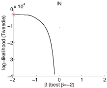
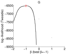
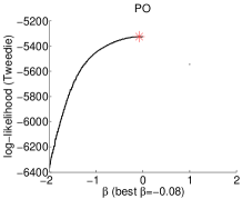
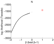
In Fig. 1 (first row), the results of the Maximum Tweedie Likelihood (MTL) are shown. The $\beta$ value that maximizes the likelihood in Tweedie distribution is consistent with the true parameters, i.e., -2, -1, 0 and 1 respectively for the above distributions. Note that Tweedie distributions are not defined for $\beta\in(0,1)$, but $\beta$-divergence is defined in this region, which will lead to discontinuity in the log-likelihood over $\beta$.

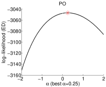
The second and third rows in Fig. 1 present results of the exponential divergence density ED given in Eq. (25). The log-likelihood and negative score matching objectives [29] on the same four datasets are shown. The estimates are consistent with the ground truth Gaussian and Poisson data. However, for Gamma and Inverse Gaussian data, both $\beta$ estimates deviate from the ground truth. Thus, estimators based on ED do not give as accurate estimates as the MTL method. The ED distribution [29] has an advantage that it is defined also for $\beta\in(0,1)$. In the above, we have seen that $\beta$ selection by using ED is accurate when $\beta\rightarrow 0$ or $\beta=1$. However, as explained in Section III-A2, in the other cases ED and Tweedie distributions are not the same because the terms containing the observed variable in these distributions are not exactly the same as those of the Tweedie distributions.

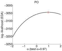
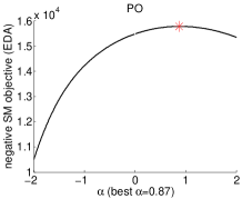
EDA, the augmented ED density introduced in Section III-A, not only has both the advantage of continuity but also gives very accurate estimates for $\beta<0$. The MEDAL log-likelihood curves over $\beta$ based on EDA are given in Fig. 1 (fourth row). In the $\beta$ selection of Eq. (24), the $\phi$ value that maximizes the likelihood with $\beta$ fixed is found by a grid search. The likelihood values are the same as those of special Tweedie distributions and there are no abrupt changes or discontinuities in the likelihood surface. We also estimated $\beta$ for the EDA density using Score Matching, and curves of the negative SM objective are presented in the bottom row of Fig. 1. They also recover the ground truth accurately.

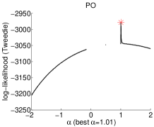
IV-A2 $\alpha$-divergence selection

There is only one known generative model for which the maximum likelihood estimator corresponds to the minimizer of the corresponding $\alpha$ divergence. It is the Poisson distribution.

(a)	(b)	(c)	(d)

Figure 2: Log-likelihood of (a) Tweedie, (b) ED, and (c) EDA distributions for $\alpha$-selection. In the Tweedie plot, blanks correspond to $\beta=1/\alpha-1$ values for which a Tweedie distribution pdf does not exist or cannot be evaluated, i.e., $\beta\in(0,1)\cup(1,\infty)$. In (d), negative SM objective function values are plotted for EDA.

We thus reused the Poisson-distributed data of the previous experiments with the $\beta$-divergence. In Fig. 2a, we present the log-likelihood objective over $\alpha$ obtained with Tweedie distribution (MTL) and the transformation from Section III-B. The ground truth $\alpha\rightarrow 1$ is successfully recovered with MTL. However, there are no likelihood estimates for $\alpha\in(0.5,1)$, corresponding to $\beta\in(0,1)$ for which no Tweedie distributions are defined. Moreover, to our knowledge there are no studies concerning the pdf’s of Tweedie distributions with $\beta>1$. For that reason, the likelihood values for $\alpha\in[0,0.5)$ are left blank in the plot.

It can be seen from Fig. 2b and 2c, that the augmentation in the MEDAL method also helps in $\alpha$ selection. Again, both ED and EDA solve most of the discontinuity problem except $\alpha=0$. Selection using ED fails to find the ground truth which equals 1, which is however successfully found by the MEDAL method. SM on EDA recovers the ground truth as well (Fig. 2d).

IV-B Divergence selection in NMF

The objective in nonnegative matrix factorization (NMF) is to find a low-rank approximation to the observed data by expressing it as a product of two nonnegative matrices, i.e., $\mathbf{V}\approx\widehat{\mathbf{V}}=\mathbf{W}\mathbf{H}$ with $\mathbf{V}\in\mathbb{R}_{+}^{F\times N}$ , $\mathbf{W}\in\mathbb{R}_{+}^{F\times K}$ and $\mathbf{H}\in\mathbb{R}_{+}^{K\times N}$. This objective is pursued through the minimization of an information divergence between the data and the approximation, i.e., $D(\mathbf{V}||\widehat{\mathbf{V}})$. The divergence can be any appropriate one for the data/application such as $\beta$, $\alpha$, $\gamma$, Rényi, etc. Here, we chose the $\beta$ and $\alpha$ divergences to illustrate the MEDAL method for realistic data.

The optimization of $\beta$-NMF was implemented using the standard multiplicative update rules [23, 38]. Similar multiplicative update rules are also available for $\alpha$-NMF [23]. Alternatively, the algorithm for $\beta$-NMF can be used for $\alpha$-divergence minimization as well, using the transformation explained in Section III-B.

IV-B1 A Short Piano Excerpt

We consider the piano data used in [21]. It is an audio sequence recorded in real conditions, consisting of four notes played all together in the first measure and in all possible pairs in the subsequent measures. A power spectrogram with analysis window of size 46 ms was computed, leading to $F=513$ frequency bins and $N=676$ time frames. These make up the data matrix $\mathbf{V}$, for which a matrix factorization $\widehat{\mathbf{V}}=\mathbf{W}\mathbf{H}$ with low rank $K=6$ is sought for.

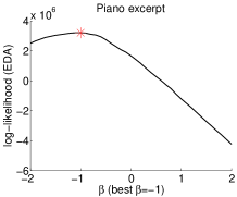
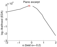
In Fig. 3a and 3b, we show the log-likelihood values of the MEDAL method for $\beta$ and $\alpha$, respectively. For each parameter value $\beta$ and $\alpha$, the multiplicative algorithm for the respective divergence is run for 100 iterations and likelihoods are evaluated with mean values calculated from the returned matrix factorizations. For each value of $\beta$ and $\alpha$, the highest likelihood w.r.t. $\phi$ (see Eq. (24)) is found by a grid search.

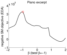
The found maximum likelihood estimate $\beta=-1$ corresponds to Itakura-Saito divergence, which is in harmony with the empirical results presented in [21] and the common belief that IS divergence is most suitable for audio spectrograms. The optimal $\alpha$ value value was 0.5 corresponding to Hellinger distance. We can also see that the log likelihood value associated with $\alpha=0.5$ is still much less than the one for $\beta=-1$. SM also finds $\beta=-1$ as can be seen from Fig. 3c.

a) $\beta$ div.	b) $\alpha$ div.
c) $\beta$ div.

Figure 3: (a, b) Log likelihood values for $\beta$ and $\alpha$ for the spectrogram of a short piano excerpt with $F=513$, $N=676$, $K=6$. (c) Negative SM objective for $\beta$.

IV-C Stock Prices

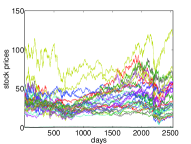
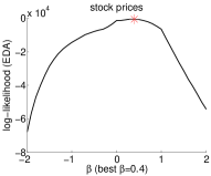
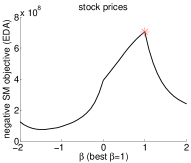
Next, we repeat the same experiment on a stock price dataset which contains Dow Jones Industrial Average. There are 30 companies included in the data. They are major American companies from various sectors such as services (e.g., Walmart), consumer goods (e.g., General Motors) and healthcare (e.g., Pfizer). The data was collected from 3rd January 2000 to 27th July 2011, in total 2543 trading dates. We set $K=5$ in NMF and masked 50% of the data by following [39]. The stock data curves are displayed in Fig. 4 (left).

The EDA likelihood curve with $\beta\in[-2,2]$ is shown in Figure 4 (bottom left). We can see that the best divergence selected by MEDAL is $\beta=0.4$. The corresponding best $\phi=0.006$. These results are in harmony with the findings of Tan and Févotte [39] using the remaining 50% of the data as validation set, where they found that $\beta\in[0,0.5]$ (mind that our $\beta$ values equal theirs minus one) performs well for a large range of $\phi$’s. Differently, our method is more advantageous because we do not need additional criteria nor data for validations. In Figure 4 (bottom right), negative SM objective function is plotted for $\beta\in[-2,2]$. With SM, the optimal $\beta$ is found to be 1.

Figure 4: Top: the stock data. Bottom left: the EDA log-likelihood for $\beta\in[-2,2]$. Bottom right: negative SM objective function for $\beta\in[-2,2]$.

IV-D Selecting $\gamma$-divergence

In this section we demonstrate that the proposed method can be applied to applications beyond NMF and to non-separable divergence families. To our knowledge, no other existing methods can handle these two cases.

IV-D1 Multinomial data

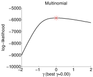
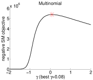
We first exemplify $\gamma$-divergence selection for synthetic data drawn from a multinomial distribution. We generated a 1000-dimensional stochastic vector $\mathbf{p}$ from the uniform distribution. Next we drew $\mathbf{x}\sim\text{Multinomial}(n,\mathbf{p})$ with $n=10^{7}$. The MEDAL method is applied to find the best $\gamma$-divergence for the approximation of $\mathbf{x}$ by $\mathbf{p}$.

Fig. 6 (1st row, left) shows the MEDAL log-likelihood. The peak appears when $\gamma=0$, which indicates that the normalized KL-divergence is the most suitable one among the $\gamma$-divergence family. Selection using score matching of EDA gives the best $\gamma$ also close to zero (Fig. 6 1st row, right). The result is expected, because the maximum likelihood estimator of $\mathbf{p}$ in multinomial distribution is equivalent to minimizing the KL-divergence over $\mathbf{p}$. Our finding also justifies the usage of KL-divergence in topic models with the multinomial distribution [40, 7].

IV-D2 Projective NMF

Next we apply the MEDAL method to Projective Nonnegative Matrix Factorization (PNMF) [27, 28] based on $\gamma$-divergence [13, 19]. Given a nonnegative matrix $\mathbf{V}\in\mathbb{R}_{+}^{F\times N}$, PNMF seeks a low-rank nonnegative matrix $\mathbf{W}\in\mathbb{R}_{+}^{F\times K}$ ($K<F$) that minimizes $D_{\gamma}\left(\mathbf{V}||\widehat{\mathbf{V}}\right)$, where $\widehat{\mathbf{V}}=\mathbf{W}\mathbf{W}^{T}\mathbf{V}$. PNMF is able to produce a highly orthogonal $\mathbf{W}$ and thus finds its applications in part-based feature extraction and clustering analysis, etc. Different from conventional NMF (or linear NMF) where each factorizing matrix only appears once in the approximation, the matrix $\mathbf{W}$ occurs twice in $\widehat{\mathbf{V}}$. Thus it is a special case of Quadratic Nonnegative Matrix Factorization (QNMF) [41].

We choose PNMF for two reasons: 1) we demonstrate the MEDAL performance on QNMF besides the linear NMF already shown in Section IV-B; 2) PNMF contains only one variable matrix in learning, without the issue of how to interleave the updates of different variable matrices.

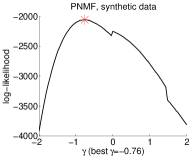
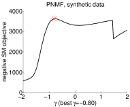
We first tested MEDAL on a synthetic dataset. We generated a diagonal blockwise data matrix $\mathbf{V}$ of size $50\times 30$, where two blocks are of sizes $30\times 20$ and $20\times 10$. The block entries are uniformly drawn from $[0,10]$. We then added uniform noise from $[0,1]$ to the all matrix entries. For each $\gamma$, we ran the multiplicative algorithm of PNMF by Yang and Oja [28, 42] to obtain $\mathbf{W}$ and $\widehat{\mathbf{V}}$. The MEDAL method was then applied to select the best $\gamma$. The resulting approximated log-likelihood for $\gamma\in[-2,2]$ is shown in Fig. 6 (2nd row). We can see MEDAL and score matching of EDA give similar results, where the best $\gamma$ appear at $-0.76$ and $-0.8$, respectively. Both resulting $W$’s give perfect clustering accuracy of data rows.

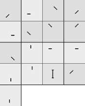
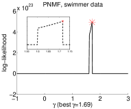
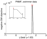
We also tested MEDAL on the swimmer dataset [43] which is popularly used in the NMF field. Some example images from this dataset are shown in Fig. 5 (left). We vectorized each image in the dataset as a column and concatenated the columns into a $1024\times 256$ data matrix $\mathbf{V}$. This matrix is then fed to PNMF and MEDAL as in the case for the synthetic dataset. Here we empirically set the rank to $K=17$ according to Tan and Févotte [44] and Yang et al. [45]. The matrix $\mathbf{W}$ was initialized by PNMF based on Euclidean distance to avoid poor local minima. The resulting approximated log-likelihood for $\gamma\in[-1,3]$ is shown in Figure 6 (3rd row, left). We can see a peak appearing around $1.7$. Zooming in the region near the peak shows the best $\gamma=1.69$. The score matching objective over $\gamma$ values (Fig. 6 3rd row, right) shows a similar peak and the best $\gamma$ very close to the one given by MEDAL. Both methods result in excellent and nearly identical basis matrix ($\mathbf{W}$) of the data, where the swimmer body as well as four limbs at four angles are clearly identified (see Fig. 5 bottom row).

Figure 5: Swimmer dataset: (top) example images; (bottom) the best PNMF basis ($\mathbf{W}$) selected by using (bottom left) MEDAL and (bottom right) score matching of EDA. The visualization reshapes each column of $\mathbf{W}$ to an image and displays it by the Matlab function imagesc.

IV-D3 Symmetric Stochastic Neighbor Embedding

Finally, we show an application beyond NMF, where MEDAL is used to find the best $\gamma$-divergence for the visualization using Symmetric Stochastic Neighbor Embedding (s-SNE) [5, 6].

Suppose there are $n$ multivariate data samples $\left\{\mathbf{x}_{i}\right\}_{i=1}^{n}$ with $\mathbf{x}_{i}\in\mathbb{R}^{D}$ and their pairwise similarities are represented by an $n\times n$ symmetric nonnegative matrix $\mathbf{P}$ where $P_{ii}=0$ and $\sum_{ij}P_{ij}=1$. The s-SNE visualization seeks a low-dimensional embedding $\mathbf{Y}=\left[\mathbf{y}_{1},\mathbf{y}_{2},\dots,\mathbf{y}_{n}\right]^{T}\in\mathbb{R}^{n\times d}$ such that pairwise similarities in the embedding approximate those in the original space. Generally $d=2$ or $d=3$ for easy visualization. Denote $q_{ij}=q(\|\mathbf{y}_{i}-\mathbf{y}_{j}\|^{2})$ with a certain kernel function $q$, for example $q_{ij}=\left(1+\|\mathbf{y}_{i}-\mathbf{y}_{j}\|^{2}\right)^{-1}$. The pairwise similarities in the embedding are then given by $Q_{ij}=q_{ij}/\sum_{kl:k\neq l}q_{kl}$. The s-SNE target is that $\mathbf{Q}$ is as close to $\mathbf{P}$ as possible. To measure the dissimilarity between $\mathbf{P}$ and $\mathbf{Q}$, the conventional s-SNE uses the Kullback-Leibler divergence $D_{\text{KL}}(\mathbf{P}||\mathbf{Q})$. Here we generalize s-SNE to the whole family of $\gamma$-divergences as dissimilarity measures and select the best divergence by our MEDAL method.

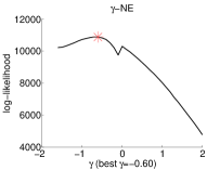
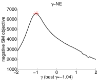
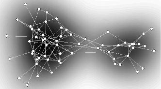
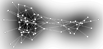
We have used a real-world dolphins dataset. It is the adjacency matrix of the undirected social network between 62 dolphins. We smoothed the matrix by PageRank random walk in order to find its macro structures. The smoothed matrix was then fed to s-SNE based on $\gamma$-divergence, with $\gamma\in[-2,2]$. The EDA log-likelihood is shown in Fig. 6 (4th row, left). By the MEDAL principle the best divergence is $\gamma=-0.6$ for s-SNE and the dolphins dataset. Score matching of EDA also indicates the best $\gamma$ is smaller than 0. The resulting visualizations created by s-SNE with the respective best $gamma$-divergence are shown in Fig. 7, where the node layouts by both methods are very similar. In both visualizations we can clearly see two dolphin communities.

Figure 6: Selecting the best $\gamma$-divergence: (1st row) for multinomial data, (2nd row) in PNMF for synthetic data, (3rd row) in PNMF for the swimmer dataset, and (4th row) in s-SNE for the dolphins dataset; (left column) using MEDAL and (right column) using score matching of EDA. The red star highlights the peak and the small subfigures in each plot shows the zoom-in around the peak. The sub-figures in the 3rd row zoom in the area near the peaks.

Figure 7: Visualization of the dolphins social network with the best $\gamma$ using (top) MEDAL and (bottom) score matching of EDA. Dolphins and their social connections are shown by circles and lines, respectively. The background illustrates the node density by the Parzen method [46].

V Conclusions

We have presented a new method called MEDAL to automatically select the best information divergence in a parametric family. Our selection method is built upon a statistical learning approach, where the divergence is learned as the result of standard density parameter estimation. Maximizing the likelihood of the Tweedie distribution is a straightforward way for selecting $\beta$-divergence, which however has some shortcomings. We have proposed a novel distribution, the Exponential Divergence with Augmentation (EDA), which overcomes these shortcomings and thus can give a more robust selection for the parameter over a wider range. The new method has been extended to $\alpha$-divergence selection by a nonlinear transformation. Furthermore, we have provided new results that connect the $\gamma$- and $\beta$-divergences, which enable us to extend the selection method to non-separable cases. The extension also holds for Rényi divergence with similar relationship to $\alpha$-divergence. As a result, our method can be applied to most commonly used information divergences in learning.

We have performed extensive experiments to show the accuracy and applicability of the new method. Comparison on synthetic data has illustrated that our method is superior to Maximum Tweedie Likelihood, i.e., it finds the ground truth as accurately as MTL, while being defined on all values of $\beta$ and being less prone to numerical problems (no abrupt changes in the likelihood). We also showed that a previous estimation approach by Score Matching on Exponential Divergence distribution (ED, i.e., EDA before augmentation) is not accurate, especially for $\beta<0$. In the application to NMF, we have provided experimental results on various kinds of data including audio and stock prices. In the non-separable cases, we have demonstrated selecting $\gamma$-divergence for synthetic data, Projective NMF, and visualization by s-SNE. In those cases where the correct parameter value is known in advance for the synthetic data, or there is a wide consensus in the application community on the correct parameter value for real-world data, the MEDAL method gives expected results. These results show that the presented method has not only broad applications but also accurate selection performance. In the case of new kinds of data, for which the appropriate information divergence is not known, the MEDAL method provides a disciplined and rigorous way to compute the optimal parameter values.

In this paper we have focused on information divergence for vectorial data. There exist other divergences for higher-order tensors, for example, LogDet divergence and von Newmann divergence (see e.g. [47]) that are defined over eigenvalues of matrices. Selection among these divergences remains an open problem.

Here we mainly consider a positive data matrix and selecting the divergence parameter in $(\infty,+\infty)$. Tweedie distribution has no support for zero entries when $\beta<0$ and thus gives zero likelihood of the whole matrix/tensor by independence. In future work, extension of EDA to accommodate nonnegative data matrices could be developed for $\beta\geq 0$.

MEDAL is a two-phase method: the $\beta$ selection is based on the optimization result of $\bm{\mu}$. Ideally, both variables should be selected by optimizing the same objective. For maximum log-likelihood estimator, this requires that the negative log-likelihood equals the $\beta$-divergence, which is however infeasible for all $\beta$ due to intractability of integrals. Non-ML estimators could be used to attack this open problem.

The EDA distribution family includes the exact Gaussian, Gamma, and Inverse Gaussian distributions, and approximated Poisson distribution. In the approximation we used the first-order Stirling expansion. One could apply higher-order expansions to improve the approximation accuracy. This could be implemented by further augmentation with higher-order terms around $\beta\rightarrow 0$.

VI Acknowledgment

This work was financially supported by the Academy of Finland (Finnish Center of Excellence in Computational Inference Research COIN, grant no 251170; Zhirong Yang additionally by decision number 140398).

Appendix A Infinite series expansion in Tweedie distribution

In the series expansion, an EDM random variable is represented as a sum of $G$ independent Gamma random variables $x=\sum_{g}^{G}y_{g}$, where $G$ is Poisson distributed with parameter $\lambda=\frac{\mu^{2-p}}{\phi(2-p)}$; and the shape and scale parameters of the Gamma distribution are $-a$ and $b$, with $a=\frac{2-p}{1-p}$ and $b=\phi(p-1)\mu^{p-1}$.

The pdf of the Tweedie distribution is obtained analytically at $x=0$ as $e^{-\frac{\mu^{2-p}}{\phi(2-p)}}$. For $x>0$ the function $f(x,\phi,p)=\frac{1}{x}\sum_{j=1}^{\infty}W_{j}(x,\phi,p)$, where for $1<p<2$

$$W_{j}=\frac{x^{-ja}(p-1)^{ja}}{\phi^{j(1-a)}(2-p)^{j}j!\Gamma(-ja)}$$ (29)

and for $p>2$

$$W_{j}=\frac{1}{\pi}\frac{\Gamma(1+ja)\phi^{j(a-1)}(p-1)^{ja}}{\Gamma(1+j)(p-1)^{j}x^{ja}}(-1)^{j}\sin(-\pi ja).$$ (30)

This infinite summation needs approximation in practice. Dunn and Smyth [35] described an approach to select a subset of these infinite terms to accurately approximate $f(x,\phi,p)$. In their approach, Stirling’s approximation of the Gamma functions are used to find the index $j$ which gives the highest value of the function. Then, in order to find the most significant region, the indices are progressed in both directions until negligible terms are reached.

Appendix B Gauss-Laguerre quadratures

This method (e.g. [48]) can evaluate definite integrals of the form

$$\int_{0}^{\infty}e^{-z}f(z)dz\approx\sum_{i}^{n}f(z_{i})w_{i},$$ (31)

where $z_{i}$ is the $i$th root of the $n$-th order Laguerre polynomial $L_{n}(z)$, and the weights are given by

$$w_{i}=\frac{z_{i}}{(n+1)^{2}L_{n}^{2}(z_{i})}.$$ (32)

The recursive definition of $L_{n}(z)$ is given by

$$L_{n+1}(z)=\frac{1}{n+1}\left[(2n+1-z)L_{n}(z)-nL_{n-1}(z)\right],$$ (33)

with $L_{0}(z)=1$ and $L_{1}(z)=1-z$. In our experiments, we used the Matlab implementation by Winckel with $n=5000$.

Appendix C Proofs of Theorems 2 and 3

Lemma 4

$\arg\min_{z}af(z)=\arg\min_{z}a\ln f(z)$ for $a\in\mathbb{R}$ and $f(z)>0$.

The proof of the lemma is simply by the monotonicity of $\ln$.

Next we prove Theorem 2. For $\beta\in\mathbb{R}\backslash\{-1,0\}$, zeroing $\frac{\partial D_{\beta}(\mathbf{x}||c\bm{\mu})}{\partial c}$ gives

$$c^{*}=\frac{\sum_{i}x_{i}\mu_{i}^{\beta}}{\sum_{i}\mu_{i}^{1+\beta}}.$$ (34)

Putting it back to $\min_{\bm{\mu}}\min_{c}D_{\beta}(\mathbf{x}||c\bm{\mu})$, we obtain:

$$\min_{\bm{\mu}}\min_{c}D_{\beta}(\mathbf{x}||c\bm{\mu})$$

$$= \min_{\bm{\mu}}\frac{1}{\beta(1+\beta)}\left[\sum_{i}x_{i}^{1+\beta}+\beta\sum_{i}\left(\frac{\sum_{j}x_{j}\mu_{j}^{\beta}}{\sum_{j}\mu_{j}^{1+\beta}}\mu_{i}\right)^{1+\beta}\right.$$

$$\left.-(1+\beta)\sum_{i}x_{i}\left(\frac{\sum_{j}x_{j}\mu_{j}^{\beta}}{\sum_{j}\mu_{j}^{1+\beta}}\mu_{i}\right)^{\beta}\right]$$

$$= \min_{\bm{\mu}}\frac{1}{\beta(1+\beta)}\left[\sum_{i}x_{i}^{1+\beta}-\frac{\left(\sum_{i}x_{i}\mu_{i}^{\beta}\right)^{1+\beta}}{\left(\sum_{j}\mu_{j}^{1+\beta}\right)^{\beta}}\right]$$

Dropping the constant, and by Lemma 4, the above is equivalent to minimizing

$$\frac{1}{\beta(1+\beta)}\left[\beta\ln\left(\sum_{j}\mu_{j}^{1+\beta}\right)-(1+\beta)\ln\left(\sum_{i}x_{i}\mu_{i}^{\beta}\right)\right]$$

Adding a constant $\frac{1}{\beta(1+\beta)}\ln\left(\sum_{i}x_{i}^{1+\beta}\right)$, the objective becomes minimizing $\gamma$-divergence (replacing $\beta$ with $\gamma$; see Eq. (• ‣ II)).

We can apply the similar technique to prove Theorem 3. For $\alpha\in\mathbb{R}\backslash\{0,1\}$, zeroing $\frac{\partial D_{\alpha}(\mathbf{x}||c\bm{\mu})}{\partial c}$ gives

$$c^{*}=\left(\frac{\sum_{i}x_{i}^{\alpha}\mu_{i}^{1-\alpha}}{\sum_{i}\mu_{i}}\right)^{1/\alpha}$$ (35)

Putting it back, we obtain

$$D_{\alpha}(\mathbf{x}||c^{*}\bm{\mu})$$ (36)

$$= \frac{1}{\alpha(1-\alpha)}\sum_{i}\left\{\alpha x_{i}+(1-\alpha)\left(\frac{\sum_{j}x_{j}^{\alpha}\mu_{j}^{1-\alpha}}{\sum_{j}\mu_{j}}\right)^{1/\alpha}\mu_{i}\right.$$ (37)

$$\left.-x_{i}^{\alpha}\left[\left(\frac{\sum_{j}x_{j}^{\alpha}\mu_{j}^{1-\alpha}}{\sum_{j}\mu_{j}}\right)^{1/\alpha}\mu_{i}\right]^{1-\alpha}\right\}$$ (38)

$$= \frac{1}{\alpha-1}\left[\sum_{i}x_{i}^{\alpha}\left(\frac{\mu_{i}}{\sum_{j}\mu_{j}}\right)^{1-\alpha}\right]^{1/\alpha}+\frac{\sum_{i}x_{i}}{1-\alpha}.$$ (39)

Dropping the constant $\frac{\sum_{i}x_{i}}{1-\alpha}$, and by Lemma 4, minimizing the above is equivalent to minimization of (for $\alpha>0$)

$$\frac{1}{\alpha-1}\ln\left[\sum_{i}x_{i}^{\alpha}\left(\frac{\mu_{i}}{\sum_{j}\mu_{j}}\right)^{1-\alpha}\right]$$ (40)

Adding a constant $\frac{\alpha}{1-\alpha}\ln\sum_{i}x_{i}$ to the above, the objective becomes minimizing Rényi-divergence (replacing $\alpha$ with $\rho$; see Eq. (9)).

The proofs for the special cases are similar, where the main steps are given below

• $\beta=\gamma\rightarrow 0$ (or $\alpha=\rho\rightarrow 1$): zeroing $\frac{\partial D_{\beta\rightarrow 0}(\mathbf{x}||c\bm{\mu})}{\partial c}$ gives $c^{*}=\frac{\sum_{i}x_{i}}{\sum_{i}\mu_{i}}$. Putting it back, we obtain $D_{\beta\rightarrow 0}(\mathbf{x}||c^{*}\bm{\mu})=\left(\sum_{i}x_{i}\right)D_{\gamma\rightarrow 0}(\mathbf{x}||\bm{\mu})$.

• $\beta=\gamma\rightarrow-1$: zeroing $\frac{\partial D_{\beta\rightarrow-1}(\mathbf{x}||c\bm{\mu})}{\partial c}$ gives $c^{*}=\frac{1}{M}\sum_{i}\frac{x_{i}}{\mu_{i}}$, where $M$ is the length of $\mathbf{x}$. Putting it back, we obtain $D_{\beta\rightarrow-1}(\mathbf{x}||c^{*}\bm{\mu})=MD_{\gamma\rightarrow-1}(\mathbf{x}||\bm{\mu})$.

• $\alpha=\rho\rightarrow 0$: zeroing $\frac{\partial D_{\alpha\rightarrow 0}(\mathbf{x}||c\bm{\mu})}{\partial c}$ gives

  $$c^{*}=\exp\left(-\frac{\sum_{i}\mu_{i}\ln\frac{\mu_{i}}{x_{i}}}{\sum_{i}\mu_{i}}\right).$$

  Putting it back, we obtain

  $$D_{\alpha\rightarrow 0}(\mathbf{x}||c^{*}\bm{\mu})=-\exp\left(-\sum_{i}\tilde{\mu}_{i}\ln\frac{\tilde{\mu}_{i}}{x_{i}}\right)+\sum_{i}x_{i},$$

  where $\tilde{\mu}_{i}=\mu_{i}/\sum_{j}\mu_{j}$. Dropping the constant $\sum_{i}x_{i}$, minimizing $D_{\alpha\rightarrow 0}(\mathbf{x}||c^{*}\bm{\mu})$ is equivalent to minimization of $\sum_{i}\tilde{\mu}_{i}\ln\frac{\tilde{\mu}_{i}}{x_{i}}$. Adding the constant $\ln\sum_{j}x_{j}$ to the latter, the objective becomes identical to $D_{\rho\rightarrow 0}(\mathbf{x}||\bm{\mu})$, i.e. $D_{\text{KL}}(\bm{\mu}||\mathbf{x})$.

References

- [1] R. Kompass, “A generalized divergence measure for nonnegative matrix factorization,” Neural Computation, vol. 19, no. 3, pp. 780–791, 2006.
- [2] I. S. Dhillon and S. Sra, “Generalized nonnegative matrix approximations with Bregman divergences,” in Advances in Neural Information Processing Systems, vol. 18, 2006, pp. 283–290.
- [3] A. Cichocki, H. Lee, Y.-D. Kim, and S. Choi, “Non-negative matrix factorization with -divergence,” Pattern Recognition Letters, vol. 29, pp. 1433–1440, 2008.
- [4] Z. Yang and E. Oja, “Unified development of multiplicative algorithms for linear and quadratic nonnegative matrix factorization,” IEEE Transactions on Neural Networks, vol. 22, no. 12, pp. 1878–1891, 2011.
- [5] G. Hinton and S. Roweis, “Stochastic neighbor embedding,” in Advances in Neural Information Processing Systems, 2002, pp. 833–840.
- [6] L. van der Maaten and G. Hinton, “Visualizing data using t-SNE,” Journal of Machine Learning Research, vol. 9, pp. 2579–2605, 2008.
- [7] D. Blei, A. Y. Ng, and M. I. Jordan, “Latent dirichlet allocation,” Journal of Machine Learning Research, vol. 3, pp. 993–1022, 2001.
- [8] I. Sato and H. Nakagawa, “Rethinking collapsed variational bayes inference for lda,” in International Conference on Machine Learning (ICML), 2012.
- [9] T. Minka, “Divergence measures and message passing,” Microsoft Research, Tech. Rep., 2005.
- [10] H. Chernoff, “A measure of asymptotic efficiency for tests of a hypothesis based on a sum of observations,” The Annals of Mathematical Statistics, vol. 23, pp. 493–507, 1952.
- [11] S. Amari, Differential-Geometrical Methods in Statistics. Springer Verlag, 1985.
- [12] A. Basu, I. R. Harris, N. Hjort, and M. Jones, “Robust and efficient estimation by minimising a density power divergence,” Biometrika, vol. 85, pp. 549–559, 1998.
- [13] H. Fujisawa and S. Eguchi, “Robust paramater estimation with a small bias against heavy contamination,” Journal of Multivariate Analysis, vol. 99, pp. 2053–2081, 2008.
- [14] A. Cichocki and S.-i. Amari, “Families of alpha- beta- and gamma- divergences: Flexible and robust measures of similarities,” Entropy, vol. 12, no. 6, pp. 1532–1568, 2010.
- [15] A. Cichocki, S. Cruces, and S.-I. Amari, “Generalized alpha-beta divergences and their application to robust nonnegative matrix factorization,” Entropy, vol. 13, pp. 134–170, 2011.
- [16] I. Csiszár, “Eine informationstheoretische ungleichung und ihre anwendung auf den beweis der ergodizitat von markoffschen ketten,” Publications of the Mathematical Institute of Hungarian Academy of Sciences Series A, vol. 8, pp. 85–108, 1963.
- [17] T. Morimoto, “Markov processes and the h-theorem,” Journal of the Physical Society of Japan, vol. 18, no. 3, pp. 328–331, 1963.
- [18] L. M. Bregman, “The relaxation method of finding the common points of convex sets and its application to the solution of problems in convex programming,” USSR Computational Mathematics and Mathematical Physics, vol. 7, no. 3, pp. 200–217, 1967.
- [19] Z. Yang, H. Zhang, Z. Yuan, and E. Oja, “Kullback-leibler divergence for nonnegative for nonnegative matrix factorization,” in Proceedings of 21st International Conference on Artificial Neural Networks, 2011, pp. 14–17.
- [20] Z. Yang and E. Oja, “Projective nonnegative matrix factorization with -divergence,” in Proceedings of 19th International Conference on Artificial Neural Networks, 2009, pp. 20–29.
- [21] C. Févotte, N. Bertin, and J.-L. Durrieu, “Nonnegative matrix factorization with the Itakura-Saito divergence. With application to music analysis,” Neural Computation, vol. 21, no. 3, pp. 793–830, 2009.
- [22] B. Jørgensen, “Exponential dispersion models,” Journal of the Royal Statistical Society. Series B (Methodological), vol. 49, no. 2, pp. 127–162, 1987.
- [23] A. Cichocki, R. Zdunek, A. H. Phan, and S. Amari, Nonnegative Matrix and Tensor Factorization. John Wiley and Sons, 2009.
- [24] Y. K. Yilmaz and A. T. Cemgil, “Alpha/beta divergences and Tweedie models,” CoRR, vol. abs/1209.4280, 2012.
- [25] A. Hyvärinen, “Estimation of non-normalized statistical models using score matching,” Journal of Machine Learning Research, vol. 6, pp. 695–709, 2005.
- [26] D. D. Lee and H. S. Seung, “Learning the parts of objects by non-negative matrix factorization,” Nature, vol. 401, pp. 788–791, 1999.
- [27] Z. Yuan and E. Oja, “Projective nonnegative matrix factorization for image compression and feature extraction,” in Proceedings of 14th Scandinavian Conference on Image Analysis, 2005, pp. 333–342.
- [28] Z. Yang and E. Oja, “Linear and nonlinear projective nonnegative matrix factorization,” IEEE Transactions on Neural Networks, vol. 21, no. 5, pp. 734–749, 2010.
- [29] Z. Lu, Z. Yang, and E. Oja, “Selecting -divergence for nonnegative matrix factorization by score matching,” in Proceedings of the 22nd International Conference on Artificial Neural Networks (ICANN 2012), 2012, pp. 419–426.
- [30] S. Eguchi and Y. Kano, “Robustifing maximum likelihood estimation,” Institute of Statistical Mathematics, Tokyo, Tech. Rep., 2001.
- [31] M. Minami and S. Eguchi, “Robust blind source separation by beta divergence,” Neural Computation, vol. 14, pp. 1859–1886, 2002.
- [32] A. Rényi, “On measures of information and entropy,” in Procedings of 4th Berkeley Symposium on Mathematics, Statistics and Probability, 1960, pp. 547–561.
- [33] M. Mollah, S. Eguchi, and M. Minami, “Robust prewhitening for ica by minimizing beta-divergence and its application to fastica,” Neural Processing Letters, vol. 25, pp. 91–110, 2007.
- [34] H. Choi, S. Choi, A. Katake, and Y. Choe, “Learning alpha-integration with partially-labeled data,” in Proc. of the IEEE International Conference on Acoustics, Speech, and Signal Processing, 2010, pp. 14–19.
- [35] P. K. Dunn and G. K. Smyth, “Series evaluation of Tweedie exponential dispersion model densities,” Statistics and Computing, vol. 15, no. 4, pp. 267–280, 2005.
- [36] ——, “Tweedie family densities: methods of evaluation,” in Proceedings of the 16th International Workshop on Statistical Modelling, 2001.
- [37] A. Hyvärinen, “Some extensions of score matching,” Comput. Stat. Data Anal., vol. 51, no. 5, pp. 2499–2512, 2007.
- [38] C. Févotte and J. Idier, “Algorithms for nonnegative matrix factorization with the beta-divergence,” Neural Computation, vol. 23, no. 9, 2011.
- [39] C. F. V. Tan, “Automatic relevance determination in nonnegative matrix factorization with the -divergence,” IEEE Transactions on Pattern Analysis and Machine Intelligence, 2013, accepted, to appear.
- [40] T. Hofmann, “Probabilistic latent semantic indexing,” in International Conference on Research and Development in Information Retrieval (SIGIR), 1999, pp. 50–57.
- [41] Z. Yang and E. Oja, “Quadratic nonnegative matrix factorization,” Pattern Recognition, vol. 45, no. 4, pp. 1500–1510, 2012.
- [42] ——, “Unified development of multiplicative algorithms for linear and quadratic nonnegative matrix factorization,” IEEE Transactions on Neural Networks, vol. 22, no. 12, pp. 1878–1891, 2011.
- [43] D. Donoho and V. Stodden, “When does non-negative matrix factorization give a correct decomposition into parts?” in Advances in Neural Information Processing Systems 16, 2003, pp. 1141–1148.
- [44] V. Y. F. Tan and C. Févotte, “Automatic relevance determination in nonnegative matrix factorization,” in Proceedings of 2009 Workshop on Signal Processing with Adaptive Sparse Structured Representations (SPARS’09), 2009.
- [45] Z. Yang, Z. Zhu, and E. Oja, “Automatic rank determination in projective nonnegative matrix factorization,” in Proceedings of the 9th International Conference on Latent Variable Analysis and Signal Separation (LVA2010), 2010, pp. 514–521.
- [46] E. Parzen, “On Estimation of a Probability Density Function and Mode,” The Annals of Mathematical Statistics, vol. 33, no. 3, pp. 1065–1076, 1962.
- [47] B. Kulis, M. A. Sustik, and I. S. Dhillon, “Low-rank kernel learning with bregman matrix divergences,” Journal of Machine Learning Research, vol. 10, pp. 341–376, 2009.
- [48] M. Abramowitz and I. A. Stegun, Eds., Handbook of Mathematical Functions with Formulas, Graphs, and Mathematical Tables, 9th ed. New York: Dover, 1972, page 890.