Model Reduction for DAEs with an Application to Flow Control

Abstract

Direct numerical simulation of dynamical systems is of fundamental importance in studying a wide range of complex physical phenomena. However, the ever-increasing need for accuracy leads to extremely large-scale dynamical systems whose simulations impose huge computational demands. Model reduction offers one remedy to this problem by producing simpler reduced models that are both easier to analyze and faster to simulate while accurately replicating the original behavior. Interpolatory model reduction methods have emerged as effective candidates for very large-scale problems due to their ability to produce high-fidelity (optimal in some cases) reduced models for linear and bilinear dynamical systems with modest computational cost. In this paper, we will briefly review the interpolation framework for model reduction and describe a well studied flow control problem that requires model reduction of a large scale system of differential algebraic equations. We show that interpolatory model reduction produces a feedback control strategy that matches the structure of much more expensive control design methodologies.

1 Introduction

Direct numerical simulation of dynamical systems has been one of the few available means for studying many complex systems of scientific and industrial value as dynamical systems are the basic framework for modeling, optimization, and control of these complex systems. Examples include chemically reacting flows, fluid dynamics, and signal propagation and interference in electric circuits. However, the ever increasing complexity and need for improved accuracy lead to the inclusion of greater detail in the model, and inevitably finer discretizations. Combined with the potential coupling to other complex systems, this results in extremely large-scale dynamical systems with millions of degrees of freedom to simulate. The simulations in these settings can be overwhelming; which is the main motivation for model reduction. The goal is to construct reduced models with significantly lower number of degrees of freedom that are easier to analyze and faster to simulate yet accurately approximate the important features in the underlying full-order large-scale simulations.

There is a tremendous amount of literature on model reduction. Here we only include a partial list of various applications settings where model reduction has been applied with great success: In fluid flow [65, 25, 32, 48, 38, 49] and design of feedback control systems [9, 11, 34, 42, 52, 53, 63], in optimization [8, 43, 4, 5, 12, 26, 75], in nonlinear inverse problems [71, 30, 45, 26, 24, 21], in optimal design [47, 46, 3], in the analysis of structural mechanics [68, 33, 51, 18, 64], in circuit theory [27, 55, 23, 19, 13, 28, 10, 62, 14], and in structural mechanics, such as [68, 33, 51, 18, 64]. For a detailed discussion of several model reduction topics, see [41, 6, 14, 15, 54].

The active flow control application we consider in this paper is a well studied flow control problem of stabilizing the von Kármán vortex shedding behind a circular cylinder by controlling the rotational velocity of the cylinder. Upon linearizing the Navier-Stokes equations about a desired steady-state solution, the resulting large-scale linear systems of differential algebraic equations (DAE) is reduced by the interpolatory model reduction framework recently developed in [35]. We use this reduced model to design the feedback control strategy and compare these results to other feedback control laws found in the literature.

2 Description of the Flow Control Problem

Suppression of the vortex shedding behind a bluff body is a classical flow control problem with numerous applications ranging from minimizing drag to reducing the cross-stream lift-induced fatigue cycling. A number of experimental and computational studies have shown the effectiveness of cylinder surface suction and zero-mass actuation to completely suppress the von Kármán vortex street at modest Reynolds numbers that are slightly higher than the critical Reynolds number (bifurcation parameter) $Re_{c}\approx 47$, cf. [58, 37], based on the cylinder diameter and inflow velocity.

An alternate strategy capitalizes on the Magnus effect produced by cylinder rotation [60]. In a sequence of experiments in [69], the authors showed that a rotationally oscillating cylinder using carefully selected choices of frequency, amplitude, and phase angle could effectively eliminate the wake for moderate flows of $Re\approx 61$ and $Re\approx 110$. At higher values of the Reynolds number, it was not possible to eliminate the wake, but using good choices of frequency and amplitude made it possible to achieve nearly 20% drag reduction. Other experimental studies [56, 29, 70] suggest that matching the oscillation frequency to the vortex shedding frequency maximizes the impact on the flow (at this range of $Re$). This was confirmed numerically in [57].

A number of active feedback control approaches for the rotating/oscillating cylinder have appeared in the literature over the past fifteen years, including [39, 74, 61, 73, 17, 20, 66, 1, 59].

In the remainder of this section we describe our feedback control strategy based on linearizing the Navier-Stokes equations about a steady-state flow and controlling the discrepancy between the actual flow and the steady-state flow (cf. [22]), discretizing the associated linear state space model and then setting up the discrete flow control problem.

The fluid flow about a rotating circular cylinder can be described using the Navier-Stokes equations

$$\frac{\partial\mathbf{v}}{\partial t}+\mathbf{v}\cdot\nabla\mathbf{v} = -\nabla{p}+\frac{1}{Re}\nabla\cdot\tau(\mathbf{v})+{\cal B}u,$$

$$\nabla\cdot\mathbf{v} = 0,$$

where $\mathbf{v}$ is the fluid velocity, $p$ is the pressure, $\tau(\mathbf{v})=\nabla\mathbf{v}+\nabla\mathbf{v}^{T}$ is the viscous stress tensor, and ${\cal B}u$ is the prescription of the Dirichlet boundary conditions on the cylinder surface with $u(t)$ representing the instantaneous tangential velocity component. Our strategy is to linearize these equations about a desired flow profile, then use this linearized model to regulate the discrepancy between the actual flow and the desired flow. For this study, we selected the steady-state solution at $Re=60$ created from a uniform free-stream velocity profile. Although the steady-state solution $(\bar{\mathbf{v}},\bar{p})$ exists at this low Reynolds number, it is an unstable equilibrium solution of the Navier-Stokes equations, solving

$$\bar{\mathbf{v}}\cdot\nabla\bar{\mathbf{v}} = -\nabla\bar{p}+\frac{1}{Re}\nabla\cdot\tau(\bar{\mathbf{v}}),$$

$$\nabla\cdot\bar{\mathbf{v}} = 0,$$

computed with uniform inflow velocity $\bar{\mathbf{v}}=(1,0)$ and zero velocity on the cylinder surface $\bar{\mathbf{v}}=\bar{u}\hat{t}=(0,0)$. For computational purposes, we consider the finite flow domain $\Omega$ consisting of the unit diameter cylinder centered at the origin embedded in a rectangular flow domain $(-7,15)\times(-7,7)$. For boundary conditions, we specify the uniform inflow velocity at the $\xi=-7$ boundary and stress-free outflow boundary conditions on the $\eta=-7$, $\xi=7$, and $\eta=7$ edges.

If we write $\mathbf{v}=\bar{\mathbf{v}}+\mathbf{v}^{\prime}$ and $p=\bar{p}+p^{\prime}$, then the flow fluctuations $(\mathbf{v}^{\prime},p^{\prime})$ satisfy the equations

$$\frac{\partial\mathbf{v}^{\prime}}{\partial t} = -\mathbf{v}^{\prime}\cdot\nabla\bar{\mathbf{v}}-\bar{\mathbf{v}}\cdot\nabla\mathbf{v}^{\prime}-\nabla p^{\prime}+\frac{1}{Re}\nabla\cdot\tau(\mathbf{v}^{\prime})+{\cal B}u+{\bf F}(\mathbf{v}^{\prime})$$ (1)

$$0 = \nabla\cdot\mathbf{v}^{\prime},$$ (2)

where ${\bf F}(\mathbf{v}^{\prime})$ satisfies $\|{\bf F}(\mathbf{v}^{\prime})\|=O(\|\mathbf{v}^{\prime}\|^{2})$. The velocity fluctuation satisfies homogeneous boundary conditions at $\xi=-7$ and stress-free boundary conditions on the remaining exterior boundaries. Using ${\cal B}u(\cdot)$ to drive $\mathbf{v}^{\prime}\rightarrow\mathbf{0}$ is equivalent to using ${\cal B}u(\cdot)$ to control the flow $(\mathbf{v},p)$ to $(\bar{\mathbf{v}},\bar{p})$. We seek to achieve this using linear control theory. Note that ignoring the nonlinear term ${\bf F}(\mathbf{v}^{\prime})$ in (1) produces the Oseen equations and often arises when developing linear feedback flow control strategies for the Navier-Stokes equations, cf. [22].

At this point, we follow the standard strategy for calculating the linear feedback control laws for this problem (known as the reduce-then-control approach). We first develop a suitable discretization for equations (1)–(2) which results in a large system of DAEs and formulate the associated linear control problem for this approximate model. The solution to the resulting control problem is challenging and typically requires the use of suitable model reduction methods. The presentation of a new model reduction strategy for this class of problems will then be provided in Section 3.2.

2.1 Finite Element Discretization and the DAE Control Problem

We use a standard Taylor-Hood (P2-P1) finite element pair to find approximations to both $(\bar{\mathbf{v}},\bar{p})$ and $(\mathbf{v}^{\prime},p^{\prime})$, cf. [36]. The nodal values of the fluctuating velocity components are denoted by $\mathbf{x}_{1}(t)$ while those for the pressure are denoted by $\mathbf{x}_{2}(t)$. We considered several choices for the controlled output variable $y$, but for the computations below, we define

$$y_{[2i-1,2i]}(t)=\frac{1}{|\Omega_{i}|}\int_{\Omega_{i}}\mathbf{v}^{\prime}(t,\xi)\ d\xi\ d\eta,\qquad t>0,$$ (3)

for six different patches downstream of the cylinder, located at $\Omega_{1}=[1,2.5]\times[0,2]$, $\Omega_{2}=[2.5,4]\times[0,2]$, $\Omega_{3}=[4,5.5]\times[0,2]$, and three more reflected about the $\xi$ axis. For each patch, we recover two components of the average fluctuating velocity. This is discretized as

$$\mathbf{y}(t)=\mathbf{C}_{1}\mathbf{x}_{1}(t)\qquad(\mbox{and generally }\mathbf{y}(t)=\mathbf{C}\mathbf{x}+\mathbf{D}\mathbf{u}),$$

and leads to $p=12$ controlled output variables.

We now describe the flow control problem as well as the discretized version, the DAE control problem. The ultimate objective is to minimize the average fluctuation of the velocity from the smooth steady-state flow by optimally prescribing the rotational motion of the cylinder. For well-posedness, we place a penalty on activating the control. Thus, the control problem is

$$\min_{u}\int_{0}^{\infty}\left\{\mathbf{y}^{T}(t)\mathbf{y}(t)+u^{T}(t)Ru(t)\right\}\ dt,$$

where $R>0$ is a preselected constant (taken as 10 in this study), and subject to the constraint that the flow satisfies (1)–(2) from some initial perturbed flow state.

Upon discretization, the problem becomes: Find a control $\mathbf{u}(\cdot)$ that solves

$$\min_{\mathbf{u}}\int_{0}^{\infty}\left\{\mathbf{x}_{1}^{T}(t)\mathbf{C}_{1}^{T}\mathbf{C}_{1}\mathbf{x}_{1}(t)+\mathbf{u}^{T}(t)\mathbf{R}\mathbf{u}(t)\right\}\ dt,$$ (4)

subject to

$$\left[\begin{array}[]{cc}\mathbf{E}_{11}&\mathbf{0}\\ \mathbf{0}&\mathbf{0}\end{array}\right]\left[\begin{array}[]{c}\dot{\mathbf{x}}_{1}(t)\\ \dot{\mathbf{x}}_{2}(t)\end{array}\right]=\left[\begin{array}[]{cc}\mathbf{A}_{11}&\mathbf{A}_{21}^{T}\\ \mathbf{A}_{21}&\mathbf{0}\end{array}\right]\left[\begin{array}[]{c}\mathbf{x}_{1}(t)\\ \mathbf{x}_{2}(t)\end{array}\right]+\left[\begin{array}[]{c}\mathbf{B}_{1}\\ \mathbf{0}\end{array}\right]\mathbf{u}(t),$$ (5)

where $\mathbf{E}_{11}\in\bbbr^{n_{1}\times n_{1}}$ is the mass matrix for the velocity fluctuation variables and has full rank. The matrix $\mathbf{A}_{11}\in\bbbr^{n_{1}\times n_{1}}$, $\mathbf{A}_{21}\in\bbbr^{n_{2}\times n_{1}}$, and $\mathbf{B}_{1}\in\bbbr^{n_{1}\times m}$ (note that we use the Dirichlet map, cf. [44], and $m=1$ for this problem). Since we consider stress-free outflow conditions, ${\mathbf{A}}_{21}$ has full rank and ${\mathbf{A}}_{21}{\mathbf{E}}_{11}^{-1}{\mathbf{A}}_{21}^{T}$ is nonsingular. Additionally, since the tangential velocity control doesn’t add mass to the domain, the term $\mathbf{B}_{2}$ does not appear above.

To capture the von Kármán vortex street, as well as to resolve the influence of cylinder rotations on the flow for this modest Reynolds number of 60, we use a mesh with about 5,400 elements. However, in most flow control problems, typical dimensions of $n_{1}$ and $n_{2}$ prohibit the straight-forward application of linear control methods to the problem above. Therefore, we investigate the use of interpolatory model reduction methods to create modest size problems from which we can develop suitable feedback control laws.

3 Interpolatory Projections

In this section, we describe the details of the interpolatory model reduction methodology we employ. We will explain the interpolation techniques for both the general DAE framework and the index-$2$ Oseen model arising in our application as explained in Section 2.

3.1 Interpolatory Model Reduction of DAEs

Consider the following system of differential algebraic equations (DAEs) given in the state-space form:

$$\begin{array}[]{rcl}{\mathbf{E}}\,\dot{{\mathbf{x}}}(t)&=&{\mathbf{A}}{\mathbf{x}}(t)+{\mathbf{B}}{\mathbf{u}}(t),\\ {\mathbf{y}}(t)&=&{\mathbf{C}}{\mathbf{x}}(t)+{\mathbf{D}}{\mathbf{u}}(t),\end{array}$$ (6)

where ${\mathbf{x}}(t)\in\mbox{\Bb R}^{n}$ represent the internal variables, ${\mathbf{u}}(t)\in\mbox{\Bb R}^{m}$ are the inputs (excitation) and ${\mathbf{y}}(t)\in\mbox{\Bb R}^{p}$ are the outputs (observation) of the underlying dynamical system. In (6), ${\mathbf{E}}\in\mbox{\Bb R}^{n\times n}$ is a singular matrix, thus leading to a DAE system, ${\mathbf{A}}\in\mbox{\Bb R}^{n\times n}$, ${\mathbf{B}}\in\mbox{\Bb R}^{n\times m}$, ${\mathbf{C}}\in\mbox{\Bb R}^{p\times n}$, and ${\mathbf{D}}\in\mbox{\Bb R}^{p\times m}$. The model reduction framework for linear dynamical systems, especially for the interpolatory methods, is best understood in the frequency domain. Towards this goal, let $\widehat{{\mathbf{u}}}(s)$ and $\widehat{{\mathbf{y}}}(s)$ denote the Laplace transforms of ${\mathbf{u}}(t)$ and ${\mathbf{y}}(t)$, respectively, and take the Laplace transformation of (6) to obtain

$$\widehat{{\mathbf{y}}}(s)={\mathbf{G}}(s)\widehat{{\mathbf{u}}}(s),\mbox{~{}where~{}}{\mathbf{G}}(s)={\mathbf{C}}(s{\mathbf{E}}-{\mathbf{A}})^{-1}{\mathbf{B}}+{\mathbf{D}}.$$ (7)

In (7), ${\mathbf{G}}(s)$ is called the transfer function of (6). We will denote both the underlying dynamical system and its transfer function by ${\mathbf{G}}$.

In this setting of model reduction, the goal is to construct a reduced model of the form

$$\begin{array}[]{rcl}{\widetilde{{\mathbf{E}}}}\,\dot{\widetilde{{\mathbf{x}}}}(t)&=&{\widetilde{{\mathbf{A}}}}\widetilde{{\mathbf{x}}}(t)+{\widetilde{{\mathbf{B}}}}{\mathbf{u}}(t),\\ \widetilde{{\mathbf{y}}}(t)&=&{\widetilde{{\mathbf{C}}}}\widetilde{{\mathbf{x}}}(t)+{\widetilde{{\mathbf{D}}}}{\mathbf{u}}(t),\end{array}$$ (8)

where ${\widetilde{{\mathbf{E}}}},{\widetilde{{\mathbf{A}}}}\in\mbox{\Bb R}^{r\times r}$, ${\widetilde{{\mathbf{B}}}}\in\mbox{\Bb R}^{r\times m}$, ${\widetilde{{\mathbf{C}}}}\in\mbox{\Bb R}^{p\times r}$, and ${\widetilde{{\mathbf{D}}}}\in\mbox{\Bb R}^{p\times m}$ with $r\ll n$ such that the reduced model output $\widetilde{{\mathbf{y}}}(t)$ approximates the original output ${\mathbf{y}}(t)$ for a wide range of input selections ${\mathbf{u}}(t)$ with bounded energy. As for the full model, we obtain the transfer function of the reduced model by taking the Laplace transform of (8):

$${\widetilde{{\mathbf{G}}}}(s)={\widetilde{{\mathbf{C}}}}(s{\widetilde{{\mathbf{E}}}}-{\widetilde{{\mathbf{A}}}})^{-1}{\widetilde{{\mathbf{B}}}}+{\widetilde{{\mathbf{D}}}}.$$ (9)

Thus, in the frequency domain, we can view the model reduction problem as a rational approximation problem in which we search for a reduced order rational function ${\widetilde{{\mathbf{G}}}}(s)$ to approximate the full order one ${\mathbf{G}}(s)$.

We will employ the commonly used Petrov-Galerkin projection framework to obtain the reduced model. We will construct two model reduction bases ${\mathbf{V}}\in\mbox{\Bb R}^{n\times r}$ and ${\mathbf{W}}\in\mbox{\Bb R}^{n\times r}$, approximate the full-order state ${\mathbf{x}}(t)$ by ${\mathbf{V}}\widetilde{{\mathbf{x}}}(t)$, and obtain the reduced-order model in (8) using

$${\widetilde{{\mathbf{E}}}}={\mathbf{W}}^{T}{\mathbf{E}}{\mathbf{V}},\quad{\widetilde{{\mathbf{A}}}}={\mathbf{W}}^{T}{\mathbf{A}}{\mathbf{V}},\quad{\widetilde{{\mathbf{B}}}}={\mathbf{W}}^{T}{\mathbf{B}},\quad\mbox{and }\quad{\widetilde{{\mathbf{C}}}}={\mathbf{C}}{\mathbf{V}}.$$ (10)

The feedthrough term ${\widetilde{{\mathbf{D}}}}$ will be chosen appropriately to enforce matching around $s=\infty$. For the case of ordinary differential equations (ODEs) where ${\mathbf{E}}$ is nonsingular, the generic choice is ${\widetilde{{\mathbf{D}}}}={\mathbf{D}}$. However, for DAEs due to the eigenvalue of the matrix pencil $\lambda{\mathbf{E}}-{\mathbf{A}}$ at infinity, special care is needed in choosing ${\widetilde{{\mathbf{D}}}}$.

3.2 Model Reduction by Rational Tangential Interpolation

In model reduction by tangential interpolation, the goal is to construct a reduced transfer function ${\widetilde{{\mathbf{G}}}}(s)$ that interpolates ${\mathbf{G}}(s)$ at selected points in the complex plane along selected directions. The interpolation data consists of the interpolation points $\{\sigma_{i}\}_{i=1}^{r}\in\mbox{\Bb C}$ together with the left tangential directions $\{\mathbf{\mathsf{c}}_{i}\}_{i=1}^{r}\in\mbox{\Bb C}^{p}$ and the right tangential directions $\{\mathbf{\mathsf{b}}_{i}\}_{i=1}^{r}\in\mbox{\Bb C}^{m}$. The usage of the terms “left” and “right” will be clarified once we define the interpolation problem: Given ${\mathbf{G}}(s)$ and the interpolation data, find a reduced model ${\widetilde{{\mathbf{G}}}}(s)={\widetilde{{\mathbf{C}}}}(s{\widetilde{{\mathbf{E}}}}-{\widetilde{{\mathbf{A}}}})^{-1}{\widetilde{{\mathbf{B}}}}+{\widetilde{{\mathbf{D}}}}$ that satisfies, for $j=1,\ldots,r,$

$$\begin{array}[]{rcll}\mathbf{\mathsf{c}}_{i}^{T}{\mathbf{G}}(\sigma_{j})&=&\mathbf{\mathsf{c}}_{i}^{T}{\widetilde{{\mathbf{G}}}}(\sigma_{j}),\\[5.69054pt] {\mathbf{G}}(\sigma_{j})\mathbf{\mathsf{b}}_{j}&=&{\widetilde{{\mathbf{G}}}}(\sigma_{j})\mathbf{\mathsf{b}}_{j},&\mbox{and}\\[5.69054pt] \mathbf{\mathsf{c}}_{i}^{T}{\mathbf{G}}^{\prime}(\sigma_{j})\mathbf{\mathsf{b}}_{j}&=&\mathbf{\mathsf{c}}_{i}^{T}{\widetilde{{\mathbf{G}}}}^{\prime}(\sigma_{j})\mathbf{\mathsf{b}}_{j}.\end{array}$$ (11)

In other words, we require the reduced rational function ${\widetilde{{\mathbf{G}}}}(s)$ (the reduced model) to be a bitangential Hermite interpolant the original rational function ${\mathbf{G}}(s)$ (the full model). One might require interpolating higher-order derivatives of ${\mathbf{G}}(s)$ as well. Moreover, one might also choose different sets of interpolation points (i.e. the right and left interpolation points) along with the left and right tangential direction vectors. For brevity of the paper, we will consider only up to Hermite interpolation and choose one set of interpolation points. For the details of the general case, we refer the reader to [7, 35, 31].

The fundamental difference between model reduction of DAEs and ODEs is that due to the eigenvalue at infinity, the transfer function of a DAE system might contain a polynomial part. The reduced transfer function is required to exactly match the polynomial part of ${\mathbf{G}}(s)$; otherwise the error around $s=\infty$ can grow unbounded leading to unbounded model reduction error. Therefore, model reduction methods for DAEs aims to enforce matching of polynomial parts; see, e.g., [67, 50, 40, 16, 35, 2] and the references therein.

Towards this goal, let ${\mathbf{G}}(s)$ be additively decomposed as

$${\mathbf{G}}(s)={{\mathbf{G}}}_{\rm sp}(s)+{{\mathbf{P}}}(s),$$ (12)

where ${{\mathbf{G}}}_{\rm sp}(s)$ is the strictly proper rational part, i.e., $\lim_{s\to\infty}{\mathbf{G}}(s)=0$ and ${{\mathbf{P}}}(s)$ is the polynomial part of ${\mathbf{G}}(s)$. We will require that the reduced transfer function ${\widetilde{{\mathbf{G}}}}(s)$ have exactly the same polynomial part as ${\mathbf{G}}(s)$, i.e.,

$${\widetilde{{\mathbf{G}}}}(s)={\widetilde{{\mathbf{G}}}_{\rm sp}}(s)+{\widetilde{{\mathbf{P}}}}(s),\mbox{~{}~{}~{}where~{}~{}~{}}{\widetilde{{\mathbf{P}}}}(s)={{\mathbf{P}}}(s),$$

and ${\widetilde{{\mathbf{G}}}_{\rm sp}}(s)$ is the strictly proper rational part. This will guarantee that the error transfer function does not contain a polynomial part and is simply given by ${\mathbf{G}}_{\rm err}(s)={\mathbf{G}}(s)-{\widetilde{{\mathbf{G}}}}(s)={{\mathbf{G}}}_{\rm sp}(s)-{\widetilde{{\mathbf{G}}}_{\rm sp}}(s).$ For model reduction by tangential interpolation, [35, 72] showed how to construct the model reduction bases ${\mathbf{V}}$ and ${\mathbf{W}}$ so that the reduced-model of (10) satisfies the interpolation conditions (11) in addition to guaranteeing ${\widetilde{{\mathbf{P}}}}(s)={{\mathbf{P}}}(s)$. As expected, the left and right deflating subspaces of the pencil $\lambda{\mathbf{E}}-{\mathbf{A}}$ corresponding to the finite and infinite eigenvalues will play a fundamental role in achieving this goal. The next result is a special case of Theorem 3.1 in [35] simplified to Hermite interpolation.

Theorem 3.1

Given ${\mathbf{G}}(s)={\mathbf{C}}(s{\mathbf{E}}-{\mathbf{A}})^{-1}{\mathbf{B}}+{\mathbf{D}}$, let ${\mathbf{P}}_{l}$ and ${\mathbf{P}}_{r}$ be the spectral projectors onto the left and right deflating subspaces of the pencil $\lambda{\mathbf{E}}-{\mathbf{A}}$ corresponding to the finite eigenvalues. Let the columns of ${\mathbf{W}}_{\infty}$ and ${\mathbf{V}}_{\infty}$ span the left and right deflating subspaces of $\lambda{\mathbf{E}}-{\mathbf{A}}$ corresponding to the eigenvalue at infinity. Let $\sigma_{i}\in\mbox{\Bb C}$, for $i=1,\ldots,r$ be interpolation points such that $\sigma_{i}{\mathbf{E}}-{\mathbf{A}}$ and $\sigma_{i}{\widetilde{{\mathbf{E}}}}-{\widetilde{{\mathbf{A}}}}$ are nonsingular. Also let $\mathbf{\mathsf{b}}_{i}\in\mbox{\Bb C}^{m}$ and $\mathbf{\mathsf{c}}_{i}\in\mbox{\Bb C}^{p}$ be the corresponding tangential direction vectors for $i=1,\ldots,r$. Construct ${\mathbf{V}}_{\!f}$ and ${\mathbf{W}}_{\!f}$ such that

$$(\sigma_{i}{\mathbf{E}}-{\mathbf{A}})^{-1}{\mathbf{P}}_{l}{\mathbf{B}}\mathbf{\mathsf{b}}_{i} \in{\rm Im}({\mathbf{V}}_{\!f})\mbox{~{}~{}for~{}~{}}i=1,\ldots,r,$$ (13)

$$\mbox{and~{}~{}}(\sigma_{i}{\mathbf{E}}-{\mathbf{A}})^{-T}{\mathbf{P}}_{r}^{T}{\mathbf{C}}^{T}\mathbf{\mathsf{c}}_{i} \in{\rm Im}({\mathbf{W}}_{\!f})\mbox{~{}~{}for~{}~{}}i=1,\ldots,r.$$ (14)

Then with the choice of ${\mathbf{W}}=[\,{\mathbf{W}}_{\!f},\;{\mathbf{W}}_{\infty}\,]$, ${\mathbf{V}}=[\,{\mathbf{V}}_{\!f},\;{\mathbf{V}}_{\infty}\,]$, and ${\widetilde{{\mathbf{D}}}}={\mathbf{D}}$, the reduced-order model $\widetilde{{\mathbf{G}}}(s)={\widetilde{{\mathbf{C}}}}(s{\widetilde{{\mathbf{E}}}}-{\widetilde{{\mathbf{A}}}})^{-1}{\widetilde{{\mathbf{B}}}}+{\widetilde{{\mathbf{D}}}}$ obtained via projection as in (10) satisfies the bitangential Hermite interpolation conditions (11) as well as $\widetilde{{\mathbf{P}}}(s)={\mathbf{P}}(s)$.

Even though Theorem 3.1 resolves the tangential interpolation problem for DAEs, it comes with a numerical caveat that it explicitly uses the spectral projectors ${\mathbf{P}}_{r}$ and ${\mathbf{P}}_{l}$ in the model reduction step. For large-scale DAEs, computing ${\mathbf{P}}_{r}$ and ${\mathbf{P}}_{l}$ is, at best, very costly if not infeasible. Therefore, it is important to construct the model reduction bases without forming ${\mathbf{P}}_{r}$ and ${\mathbf{P}}_{l}$ explicitly. Fortunately, for the Stokes-type descriptor systems of index 2, [35, 72] recently showed how to apply interpolatory projections without forming ${\mathbf{P}}_{r}$ and ${\mathbf{P}}_{l}$ explicitly. This is what we consider next.

3.3 Interpolation Theorem for Stokes-type DAEs of Index 2

Recall the linearized DAE in (5), together with the output equation, appearing as the constraint for the optimal control problem:

$$\left[\begin{array}[]{cc}\mathbf{E}_{11}&\mathbf{0}\\ \mathbf{0}&\mathbf{0}\end{array}\right]\left[\begin{array}[]{c}\dot{\mathbf{x}}_{1}(t)\\ \dot{\mathbf{x}}_{2}(t)\end{array}\right] = \left[\begin{array}[]{cc}\mathbf{A}_{11}&\mathbf{A}_{21}^{T}\\ \mathbf{A}_{21}&\mathbf{0}\end{array}\right]\left[\begin{array}[]{c}\mathbf{x}_{1}(t)\\ \mathbf{x}_{2}(t)\end{array}\right]+\left[\begin{array}[]{c}\mathbf{B}_{1}\\ \mathbf{B}_{2}\end{array}\right]\mathbf{u}(t),$$ (25)

$${\mathbf{y}}(t) = {\mathbf{C}}_{1}{\mathbf{x}}_{1}(t)+{\mathbf{C}}_{2}{\mathbf{x}}_{2}(t)+{\mathbf{D}}{\mathbf{u}}(t),$$ (26)

where ${\mathbf{E}}_{11}$ is nonsingular, $\mathbf{B}_{2}=\mathbf{0}$, ${\mathbf{A}}_{21}$ has full rank and ${\mathbf{A}}_{21}{\mathbf{E}}_{11}^{-1}{\mathbf{A}}_{21}^{T}$ is nonsingular. In this case, system (25) is of index 2. The next theorem from [35] will show how to construct a reduced model for (25) without requiring the deflating projectors. For details of the derivations, we refer the reader to [35]. Also, for balanced-truncation based model reduction of (25), see [40].

Theorem 3.2

Given are the full-order DAE in (25), and the interpolation points $\sigma_{i}\in\mbox{\Bb C}$ together with the tangential direction vectors $\mathbf{\mathsf{b}}_{i}\in\mbox{\Bb C}^{m}$ and $\mathbf{\mathsf{c}}_{i}\in\mbox{\Bb C}^{p}$ $i=1,\ldots,r$. Let ${\mathbf{v}}_{i}$ and ${\mathbf{w}}_{i}$ solve

$$\left[\begin{array}[]{cc}\sigma_{i}{\mathbf{E}}_{11}-{\mathbf{A}}_{11}{}&~{}{\mathbf{A}}_{21}^{T}\\ {\mathbf{A}}_{21}&\mathbf{0}\end{array}\right]\left[\begin{array}[]{cc}{\mathbf{v}}_{i}\\ {\mathbf{z}}\end{array}\right]=\left[\begin{array}[]{cc}{\mathbf{B}}_{1}\mathbf{\mathsf{b}}_{i}\\ \mathbf{0}\end{array}\right],$$ (27)

and

$$\left[\begin{array}[]{cc}\sigma_{i}{\mathbf{E}}_{11}^{T}-{\mathbf{A}}_{11}^{T}{}&~{}{\mathbf{A}}_{21}^{T}\\ {\mathbf{A}}_{21}&\mathbf{0}\end{array}\right]\left[\begin{array}[]{cc}{\mathbf{w}}_{i}\\ {\mathbf{q}}\end{array}\right]=\left[\begin{array}[]{cc}{\mathbf{C}}^{T}\mathbf{\mathsf{c}}_{i}\\ \mathbf{0}\end{array}\right].$$ (28)

for $i=1,\ldots,r$. Construct

$${\mathbf{V}}=\left[{\mathbf{v}}_{1},\dots,{\mathbf{v}}_{r}\right],\mbox{~{}~{}and~{}~{}}{\mathbf{W}}=\left[{\mathbf{w}}_{1},\dots,{\mathbf{w}}_{r}\right].$$ (29)

Define

$${\widetilde{{\mathbf{D}}}}={\mathbf{D}}-{\mathbf{C}}_{2}({\mathbf{A}}_{21}{\mathbf{E}}_{11}^{-1}{\mathbf{A}}_{21}^{T})^{-1}{\mathbf{A}}_{21}{\mathbf{E}}_{11}^{-1}{\mathbf{B}}_{1}.$$

Then the reduced model

$${\widetilde{{\mathbf{G}}}}(s)={\mathbf{C}}{\mathbf{V}}(s{\mathbf{W}}^{T}{\mathbf{E}}_{11}{\mathbf{V}}-{\mathbf{W}}^{T}{\mathbf{A}}_{11}{\mathbf{V}})^{-1}{\mathbf{W}}^{T}{\mathbf{B}}_{1}+{\widetilde{{\mathbf{D}}}}.$$ (30)

satisfies the bitangential Hermite interpolation conditions (11) as well as $\widetilde{{\mathbf{P}}}(s)={\mathbf{P}}(s)$.

Note that the expensive spectral projector computations are completely avoided; the only numerical cost is the need to solve $2r$ (sparse) linear systems arising in (27) and (28).

We also note that Theorem 3.2 can be directly extended to the case where the algebraic equation in (25) has the form $\mathbf{0}={\mathbf{A}}_{21}{\mathbf{x}}_{1}(t)+{\mathbf{B}}_{2}{\mathbf{u}}(t)$ with ${\mathbf{B}}_{2}\neq\mathbf{0}$. The numerical cost stays the same; see [35, 40] for details.

4 Numerical Results

We now apply the interpolatory model reduction algorithm described in Section 3.3 to the flow control problem described in Section 2.1. A relatively coarse mesh containing 5378 triangular elements was used to discretize flow solutions in the domain $\Omega=(-7,15)\times(-7,7)\backslash c$ where $c$ is the cylinder centered at the origin with unit diameter. The steady-state flow corresponding to $Re=60$ was computed on this mesh and the resulting $(\bar{\mathbf{v}},\bar{p})$ was used to compute the discrete model for the flow fluctuations where $n_{1}=21,390$ and $n_{2}=2,777$. Plots of $\bar{\mathbf{v}}$ components appear in Fig. 1.

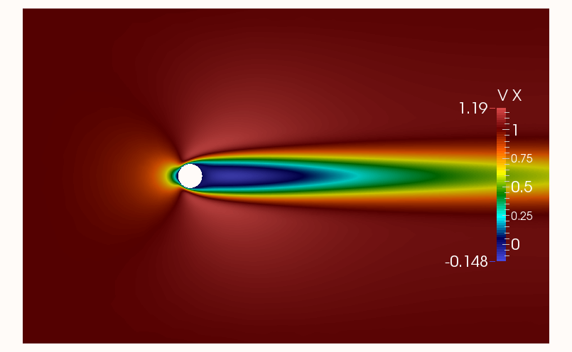
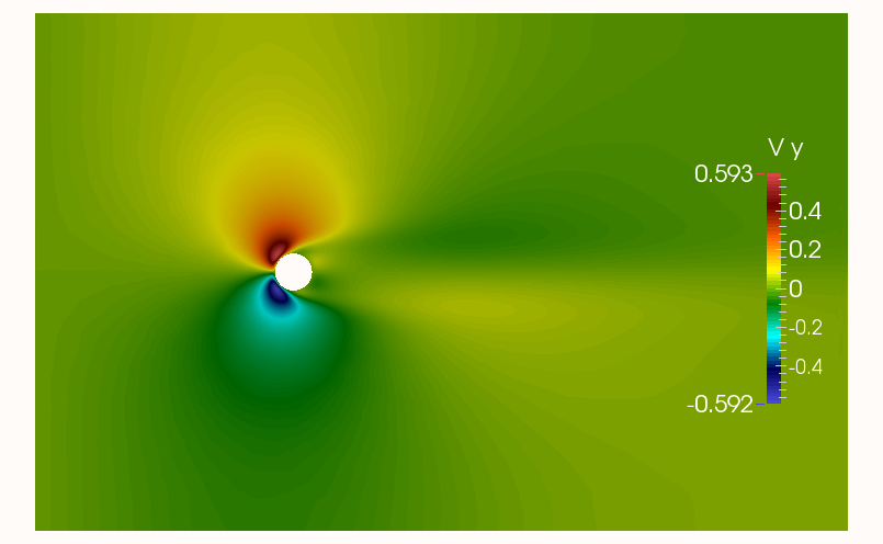
Figure 1: Steady-state velocity contours (horizontal-left, vertical-right)

As mentioned in Section 3.3, the linearization around the steady-state solution at $Re=60$ leads an unstable model; i.e the full-model DAE in (25) is unstable. There are two unstable poles are at $5.2480\times 10^{-2}\pm\imath 7.6720\times 10^{-1}$. We note that the model reduction framework we use does not require computing these unstable poles; we include them for comparison to the reduced model. The flexibility of the interpolatory model reduction is that even though the original model is unstable, Theorem 3.2 can still be applied as long as the interpolation points are not chosen as one of the poles. We have simply chosen $33$ complex conjugate pairs (overall $66$ points) on the imaginary axis as the interpolation points. The imaginary parts of the interpolation points varied from $10^{-3}$ to $10^{3}$. Then, using Theorem 3.2, we have constructed our model reduction space ${\mathbf{V}}\in\mbox{\Bb R}^{21390\times 66}$. To preserve the symmetry in ${\mathbf{E}}_{11}$, we have simply set ${\mathbf{W}}={\mathbf{V}}$. Thus, the reduced transfer function is a Lagrange interpolant in this case, not a Hermite interpolant. Due to the complex conjugate-pairs, construction of ${\mathbf{V}}$ required only $33$ sparse linear solves. Then, using a short-SVD (a relatively minor computational task due to the small number of columns in ${\mathbf{V}}$), we have removed the linear dependent columns from ${\mathbf{V}}$, and reduced the dimension to $r=60$; thus having a final reduced model of order $r=60$.

An important requirement of the reduced model in this optimal control setting is that the reduced model should capture the unstable poles of the original model so that the controller design based on the reduced model can work effectively on the full-model. As for the full-order model, our reduced model has exactly two unstable poles. The unstable poles of ${\mathbf{G}}(s)$ and ${\widetilde{{\mathbf{G}}}}(s)$ are listed below:

$$\begin{array}[]{c}\lambda_{\rm unstable}({\mathbf{G}}(s)):~{}~{}~{}5.248019596820730\times 10^{-2}\pm\imath\,7.672028760928972\times 10^{-1}\\ \lambda_{\rm unstable}({\widetilde{{\mathbf{G}}}}(s)):~{}~{}~{}5.248030491505502\times 10^{-2}\pm\imath\,7.672029050490372\times 10^{-1}\end{array}$$

As these numbers show, the unstable poles of ${\mathbf{G}}(s)$ are captured to a great accuracy as desired. To further illustrate the quality of the reduced model, in Fig. 2, we depict the singular values plots of frequency responses of ${\mathbf{G}}(s)$ and ${\widetilde{{\mathbf{G}}}}(s)$, i.e. $\|{\mathbf{G}}(\imath\omega)\|$ and $\|{\widetilde{{\mathbf{G}}}}(\imath\omega)\|$ vs $\omega\in\mbox{\Bb R}$. As the figure shows, ${\widetilde{{\mathbf{G}}}}(s)$ replicates ${\mathbf{G}}(s)$ almost exactly.

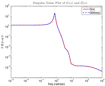
Figure 2: The singular value plots of the full-model ${\mathbf{G}}(s)$ and the reduced model ${\widetilde{{\mathbf{G}}}}(s)$

We use the reduced-order model (30) to compute an approximate solution to the LQR problem (4). Therefore, since $\widetilde{\mathbf{D}}=\mathbf{0}$ in our example, we consider the solution to the problem

$$\min_{\mathbf{u}}\int_{0}^{\infty}\widetilde{\mathbf{x}}_{1}^{T}(t)\widetilde{\mathbf{C}}_{1}^{T}\widetilde{\mathbf{C}}_{1}\widetilde{\mathbf{x}}_{1}(t)+\mathbf{u}^{T}(t)\mathbf{R}\mathbf{u}(t)\ dt$$ (31)

subject to $\widetilde{\mathbf{x}}_{1}(\cdot)$ solving (8). The solution can be computed by solving the algebraic Riccati equation (using the care function in Matlab)

$$\widetilde{\mathbf{A}}_{11}^{T}\mathbf{P}\widetilde{\mathbf{E}}_{11}+\widetilde{\mathbf{E}}_{11}^{T}\mathbf{P}\widetilde{\mathbf{A}}_{11}-\widetilde{\mathbf{E}}_{11}^{T}\mathbf{P}\widetilde{\mathbf{B}}_{1}\mathbf{R}^{-1}\widetilde{\mathbf{B}}_{1}^{T}\mathbf{P}\widetilde{\mathbf{E}}_{11}+\mathbf{\widetilde{C}}_{1}^{T}\mathbf{\widetilde{C}}_{1}=\mathbf{0}$$

for the positive definite, symmetric solution $\mathbf{P}$, then computing

$$\widetilde{\mathbf{K}}=\mathbf{R}^{-1}\widetilde{\mathbf{B}}_{1}^{T}\mathbf{P}\widetilde{\mathbf{E}}_{11}.$$

The solution to (31) is then ${\mathbf{u}}=-\widetilde{\mathbf{K}}\widetilde{\mathbf{x}}_{1}$. To find the representation of the control law in the original (full-order, discrete) variables, we can use

$${\mathbf{u}}=-\underbrace{\widetilde{\mathbf{K}}\mathbf{V}^{T}}_{\mathbf{K}}\underbrace{\mathbf{V}\widetilde{\mathbf{x}}_{1}}_{\approx\mathbf{x}_{1}}.$$

Finally, we can consider the computation of $\mathbf{u}$ as an approximation of the infinite dimensional control problem where $\mathbf{v}=(v_{\xi},v_{\eta})$ for spatial variables $(\xi,\eta)$

$$u(t)=-\int_{\Omega}h_{v_{\xi}}(\xi,\eta)(v_{\xi}(\xi,\eta,t)-\bar{v}_{\xi}(\xi,\eta))+h_{v_{\eta}}(\xi,\eta)(v_{\eta}(\xi,\eta,t)-\bar{v}_{\eta}(\xi,\eta))\ d\xi\ d\eta.$$

The finite element representations of the gains $h_{v_{\xi}}$ and $h_{v_{\eta}}$ corresponding, respectively, to the horizontal and vertical components of the velocity fluctuations are plotted in Fig. 3. These compare well to those calculated for the same problem (with a different $\mathbf{C}$ operator and slightly higher Reynolds number of 100) appearing in Fig. 4 of[1]. Considering that the gains computed in this study were computed with dramatically less computational cost emphasizes the feasibility of this approach.

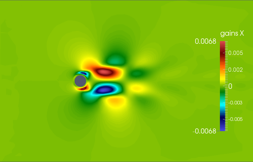
Figure 3: Functional gains (horizontal $h_{v_{\xi}}$-left, vertical $h_{v_{\eta}}$-right)

To verify that this control law stabilizes the flow, we simulated the von Kármán vortex street for 60 seconds, then applied the full-state feedback control. The control was able to nearly return the flow to the steady-state flow in 50 seconds of simulation. The control input is plotted in Fig. 4.

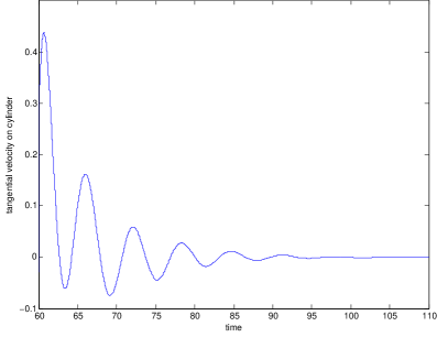
Figure 4: Control Input: Tangential Cylinder Velocity

5 Acknowledgements

We would like to thank Prof. Peter Benner for his valuable comments. This work was supported in part by the Air Force Office of Scientific Research under contract FA9550-12-1-0173 and the National Science Foundation under contracts DMS-1016450 and DMS-1217156.

6 Conclusions and Future Work

We have shown that with modest cost, using interpolatory model reduction we can produce accurate reduced models for index-$2$ DAEs arising from flow control problems. Using this model reduction framework within a control setting led to qualitatively similar functional gains as computed using more expensive control algorithms. We will apply this approach to study more complicated settings including flow control problems with higher Reynolds numbers and finer discretization. We will also investigate the practical problem of building effective state estimators and reduced-order compensators, as well as the effect of different controlled output operators on the quality of the feedback control.

References

- [1] I. Akhtar, J. Borggaard, M. Stoyanov, and L. Zietsman. On commutation of reduction and control: Linear feedback control of a von Kármán street. In Proc. 5th AIAA Flow Control Conference, Chicago, IL, 2010. AIAA Paper 2010-4832.
- [2] G. Alì, N. Banagaaya, W. Schilders, and C. Tischendorf. Index-aware model order reduction for linear index-2 DAEs with constant coefficients. SIAM Journal on Scientific Computing, 35(3):A1487–A1510, 2013.
- [3] D. Amsallem and C. Farhat. Interpolation method for the adaptation of reduced-order models to parameter changes and its application to aeroelasticity. AIAA Journal, 46:1803–1813, July 2008.
- [4] H. Antil, M. Heinkenschloss, and R. H. W. Hoppe. Domain decomposition and balanced truncation model reduction for shape optimization of the Stokes system. Optimization Methods and Software, 26(4–5):643–669, 2011.
- [5] H. Antil, M. Heinkenschloss, R. H. W. Hoppe, C. Linsenmann, and A. Wixforth. Reduced order modeling based shape optimization of surface acoustic wave driven microfluidic biochips. Mathematics and Computers in Simulation, 82(10):1986–2003, 2012.
- [6] A.C. Antoulas. Approximation of Large-Scale Dynamical Systems. SIAM Publications, Philadelphia, PA, 2005.
- [7] A.C. Antoulas, C.A. Beattie, and S. Gugercin. Interpolatory model reduction of large-scale dynamical systems. In J. Mohammadpour and K. Grigoriadis, editors, Efficient Modeling and Control of Large-Scale Systems, pages 2–58. Springer-Verlag, 2010.
- [8] E. Arian, M. Fahl, and E. Sachs. Trust-region proper orthogonal decomposition models by optimization methods. In Proceedings of the 41st IEEE Conference on Decision and Control, pages 3300–3305, Las Vegas, NV, 2002.
- [9] J. A. Atwell and B. B. King. Proper orthogonal decomposition for reduced basis feedback controllers for parabolic equations. Mathematical and Computer Modelling, 33:1–19, 2001.
- [10] Z. Bai, P. Feldmann, and R.W Freund. How to make theoretically passive reduced-order models passive in practice. In Custom Integrated Circuits Conference, pages 207–210. Proceedings of the IEEE, 1998.
- [11] H. T. Banks, S. C. Beeler, G. M. Kepler, and H. T. Tran. Reduced order modeling and control of thin film growth in an HPCVD reactor. SIAM J. on Appl. Math., 62(4), 2002.
- [12] U. Baur, P. Benner, C.A. Beattie, and S. Gugercin. Interpolatory projection methods for parameterized model reduction. SIAM Journal on Scientific Computing, 33:2489–2518, 2011.
- [13] U. Baur, P. Benner, A. Greiner, J.G. Korvink, J.Lienemann, and C. Moosmann. Parameter preserving model order reduction for MEMS applications. Mathematical and Computer Modelling of Dynamical Systems, 17(4):297–317, 2011.
- [14] P. Benner, M. Hinze, and E.J.W. ter Maten, editors. Model Reduction for Circuit Simulation, volume 74 of Lecture Notes in Electrical Engineering. Springer-Verlag, Dordrecht, NL, 2011.
- [15] P. Benner, V. L. Mehrmann, and D. C. Sorensen. Dimension Reduction of Large-scale Systems: Proceedings of a Workshop Held in Oberwolfach, Germany, October 19-25, 2003, volume 45. Springer, 2005.
- [16] P. Benner and V.I. Sokolov. Partial realization of descriptor systems. Systems & Control Letters, 55(11):929–938, 2006.
- [17] T. Bewley, J. Pralits, and P. Luchini. Minimal-energy control feedback for stabilization of bluff-body wakes based on unstable open-loop eigenvalues and left eigenvectors. In Proceedings of the Fifth Conference on Bluff Body Wakes and Vortex-Induced Vibrations (BBVIV5), pages 129–132, San Paolo, 2007.
- [18] D. S. Bindel, Z. Bai, and J. W. Demmel. Model reduction for RF MEMS simulation. In Applied Parallel Computing. State of the Art in Scientific Computing, pages 286–295. Springer, 2006.
- [19] B. N. Bond and L. Daniel. A piecewise-linear moment-matching approach to parameterized model-order reduction for highly nonlinear systems. IEEE Transactions on Computer-Aided Design of Integrated Circuits and Systems, 26(12):2116–2129, 2007.
- [20] J. Borggaard and M. Stoyanov. A reduced order solver for Lyapunov equations with high rank matrices. In Proc. 18th International Symposium on Mathematical Theory of Networks and Systems, Blacksburg, VA, 2008. Paper 169.
- [21] T. Bui-Thanh, K. Willcox, and O. Ghattas. Parametric reduced-order models for probabilistic analysis of unsteady aerodynamic applications. AIAA Journal, 46(10):2520–2529, 2008.
- [22] J. Burns. Nonlinear distributed parameter control systems with non-normal linearizations: Applications and approximations. In R.C. Smith and M.A. Demetriou, editors, Research Directions in Distributed Parameter Systems, pages 17–53. SIAM, 2003.
- [23] L. Daniel, O. C. Siong, S. C. Low, K. H. Lee, and J. White. A multiparameter moment matching model reduction approach for generating geometrically parameterized interconnect performance models. IEEE Transactions on Computer-Aided Design of Integrated Circuits and Systems, 23(5):678–693, 2004.
- [24] E. de Sturler, S. Gugercin, M. E. Kilmer, S. Chaturantabut, C. A. Beattie, and M. O’Connell. Nonlinear parametric inversion using interpolatory model reduction. arXiv preprint arXiv:1311.0922, 2013.
- [25] A. E. Deane, I. G. Kevrekidis, G. E. Karniadakis, and S. A. Orszag. Low-dimensional models for complex geometry flows: Application to grooved channels and circular cylinders. Physics of Fluids A: Fluid Dynamics, 3:2337, 1991.
- [26] V. Druskin, V. Simoncini, and M. Zaslavsky. Solution of the time-domain inverse resistivity problem in the model reduction framework part I. one-dimensional problem with SISO data. SIAM Journal on Scientific Computing, 35(3):A1621–A1640, 2013.
- [27] P. Feldmann and R.W. Freund. Efficient linear circuit analysis by Padé approximation via the Lanczos process. IEEE Transactions on Computer-Aided Design of Integrated Circuits and Systems, 14:639–649, 1995.
- [28] L. Feng. Parameter independent model order reduction. Mathematics and Computers in Simulation, 68(3):221–234, 2005.
- [29] J. R. Filler, P. L. Marston, and W. C. Mih. Response of the shear layers separating from a circular cylinder to small-amplitude rotational oscillations. Journal of Fluid Mechanics, 231:481–499, 1991.
- [30] D. Galbally, K. Fidkowski, K. Willcox, and O. Ghattas. Nonlinear model reduction for uncertainty quantification in large-scale inverse problems. International Journal for Numerical Methods in Engineering, 81(12):1581–1608, 2010.
- [31] K. Gallivan, A. Vandendorpe, and P. Van Dooren. Model reduction of MIMO systems via tangential interpolation. SIAM J. Matrix Anal. Appl., 26(2):328–349, 2005.
- [32] T. B. Gatski and M. N. Glauser. Proper orthogonal decomposition based turbulence modeling. In Instability, Transition, and Turbulence, pages 498–510. Springer, 1992.
- [33] W. Gawronski and J. Juang. Model reduction for flexible structures. Control and dynamic systems, 36:143–222, 1990.
- [34] S. Gugercin, A.C. Antoulas, C.A. Beattie, and E. Gildin. Krylov-based controller reduction for large-scale systems. In Proceedings of the 43rd IEEE Conference on Decision and Control, December 2004.
- [35] S. Gugercin, T. Stykel, and S. Wyatt. Model reduction of descriptor systems by interpolatory projection methods. SIAM Journal on Scientific Computing, 35(5):B1010–B1033, 2013.
- [36] M. Gunzburger. Finite Element Methods for Viscous Incompressible Flows. Academic Press, 1989.
- [37] M. D. Gunzburger and H. C. Lee. Feedback control of Karman vortex shedding. Transactions of the ASME, 63:828–835, 1996.
- [38] A. Hay, J. T. Borggaard, and D. Pelletier. Local improvements to reduced-order models using sensitivity analysis of the proper orthogonal decomposition. Journal of Fluid Mechanics, 629:41–72, 2009.
- [39] J. W. He, R. Glowinski, R. Metcalfe, A. Nordlander, and J. Periaux. Active control and drag optimization for flow past a circular cylinder: I. Oscillatory cylinder rotation. Journal of Computational Physics, 163:83–117, 2000.
- [40] M. Heinkenschloss, D.C. Sorensen, and K. Sun. Balanced truncation model reduction for a class of descriptor systems with application to the Oseen equations. SIAM Journal on Scientific Computing, 30(2):1038–1063, 2008.
- [41] P. Holmes, J. L. Lumley, and G. Berkooz. Turbulence, Coherent Structures, Dynamical Systems and Symmetry. Cambridge University Press, Cambridge, UK, 1996.
- [42] B. B. King. Nonuniform grids for reduced basis design of low order feedback controllers for nonlinear continuous time systems. Math. Models & Meth. in Appl. Sci., 8:1223–1241, 1998.
- [43] K. Kunisch and S. Volkwein. Proper orthogonal decomposition for optimality systems. ESAIM: Mathematical Modelling and Numerical Analysis, 42(1):1–23, 1 2008.
- [44] I. Lasiecka. Unified theory of abstract parabolic boundary problems–a semigroup approach. Applied Mathematics and Optimization, 6:287–333, 1980.
- [45] C. Lieberman, K. Willcox, and O. Ghattas. Parameter and state model reduction for large-scale statistical inverse problems. SIAM Journal on Scientific Computing, 32(5):2523–2542, August 2010.
- [46] T. Lieu and C. Farhat. Adaptation of aeroelastic reduced-order models and application to an F-16 configuration. AIAA Journal, 45(6):1244–1257, 2007.
- [47] T. Lieu, C. Farhat, and M. Lesoinne. Reduced-order fluid/structure modeling of a complete aircraft configuration. Computer Methods in Applied Mechanics and Engineering, 195:5730–5742, 2006.
- [48] H.V. Ly and H.T. Tran. Modeling and control of physical processes using proper orthogonal decomposition. Journal of Mathematical and Computer Modeling, 33:223–236, 2001.
- [49] L. Mathelin and O. Le Maitre. Robust control of uncertain cylinder wake flows based on robust reduced order models. Computers and Fluids, 38(6):1168–1182, 2009.
- [50] V. Mehrmann and T. Stykel. Balanced truncation model reduction for large-scale systems in descripter form. In P. Benner, V. Mehrmann, and D.C. Sorensen, editors, Dimension Reduction of Large-Scale Systems, volume 45 of Lecture Notes in Computational Science and Engineering, pages 83–115. Springer-Verlag, Berlin, Heidelberg, 2005.
- [51] D.G. Meyer and S. Srinivasan. Balancing and model reduction for second-order form linear systems. IEEE Transactions on Automatic Control, 41(11):1632–1644, 1996.
- [52] B. R. Noack, K. Afanasiev, M. Morzyński, G. Tadmor, and F. Thiele. A hierarchy of low-dimensional models for the transient and post-transient cylinder wake. J. Fluid Mech., 497:335–363, 2003.
- [53] B. R. Noack, G. Tadmor, and M. Morzyński. Actuation models and dissipative control in empirical Galerkin models of fluid flows. In The 2004 American Control Conference, pages 0001–0006, Boston, MA, U.S.A., June 30–July 2, 2004, 2004. Paper FrP15.6.
- [54] Goro Obinata and Brian DO Anderson. Model reduction for control system design. Springer London, 2001.
- [55] A. Odabasioglu, M. Celik, and L.T Pileggi. PRIMA: passive reduced-order interconnect macromodeling algorithm. In Proceedings of the 1997 IEEE/ACM international conference on Computer-aided design, pages 58–65, 1997.
- [56] D. J. Olinger and K. R. Sreenivasan. Nonlinear dynamics of the wake of an oscillating cylinder. Physical Review Letters, 60(9):797–800, 1988.
- [57] Y.-R. Ou. Control of oscillatory forces on a circular cylinder by rotation. Technical report, ICASE, 1991. ICASE Report No. 91–67.
- [58] D. S. Park, D. M. Ladd, and E. W. Hendricks. Feedback control of von Kármán vortex shedding behind a circular cylinder at low Reynolds numbers. Physics of Fluids, 6(7):2390–2405, 1994.
- [59] J. O. Pralits, L. Brandt, and F. Giannetti. Instability and sensitivity of the flow around a rotating circular cylinder. Journal of Fluid Mechanics, 650:513–536, 2010.
- [60] L. Prandtl. The Magnus effect and windpowered ships. Naturwissenschaften, 13:93–108, 1925.
- [61] B. Protas. Linear feedback stabilization of laminar vortex shedding based on a point vortex model. Physics of Fluids, 16:4473–4483, 2004.
- [62] T. Reis and T. Stykel. Positive real and bounded real balancing for model reduction of descriptor systems. International Journal of Control, 83(1):74–88, 2010.
- [63] C. W. Rowley, T. Colonius, and R. M. Murray. POD based models of self-sustained oscillations in the flow past an open cavity. In Proceedings of the 6th AIAA/CEAS Aeroacoustics Conference, 2000. AIAA Paper Number 2000-1969.
- [64] E. B. Rudnyi and J. G. Korvink. Review: Automatic model reduction for transient simulation of MEMS-based devices. Sensors Update, 11(1):3–33, 2002.
- [65] L. Sirovich. Turbulence and the dynamics of coherent structures. Part 1: Coherent structures. Quarterly of Applied Mathematics, 45(3):561–571, October 1987.
- [66] M. Stoyanov. Reduced Order Methods for Large Scale Riccati Equations. PhD thesis, Virginia Tech, Blacksburg, VA, May 2009.
- [67] T. Stykel. Gramian-based model reduction for descriptor systems. Mathematics of Control, Signals, and Systems, 16(4):297–319, 2004.
- [68] T.-J. Su and R.R. Craig Jr. Model reduction and control of flexible structures using Krylov vectors. Journal of Guidance, Control, and Dynamics, 14(2):260–267, 1991.
- [69] S. Taneda. Visual observations of the flow past a circular cylinder performing a rotatory oscillation. Journal of the Physical Society of Japan, 45(3):1038–1043, 1978.
- [70] P. T. Tokumaru and P. E. Dimotakis. Rotary oscillation control of a cylinder wake. Journal of Fluid Mechanics, 224:77–90, 1991.
- [71] J. Wang and N. Zabaras. Using Bayesian statistics in the estimation of heat source in radiation. International Journal of Heat and Mass Transfer, 48:15–29, 2005.
- [72] S. Wyatt. Issues in Interpolatory Model Reduction: Inexact Solves, Second-order Systems and DAEs. PhD thesis, Virginia Polytechnic Institute and State University, 2012.
- [73] M. Xiao, Y. Lin, J. H. Myatt, R. C. Camphouse, and S. S. Banda. Rotation implementation of a circular cylinder in incompressible flow via staggered grid approach. Journal of Applied Mathematics & Computing, 22(1-2):67–82, 2006.
- [74] M. Xiao, M. Novy, J. Myatt, and S. Banda. A rotary control of the circular cylinder wake: An analytic approach. In Proc. 1st AIAA Flow Control Conference, 2002. AIAA Paper 2002-3075.
- [75] Y. Yue and K. Meerbergen. Accelerating optimization of parametric linear systems by model order reduction. SIAM Journal on Optimization, 23(2):1344–1370, 2013.