Non linear evolution: revisiting the solution in the saturation region

Abstract:

In this paper we revisit the problem of the solution to Balitsky-Kovchegov equation deeply in the saturation domain. We find that solution has the form given in Ref.[9] but it depends on variable $\bar{z}=\ln(r^{2}Q^{2}_{s})+\mbox{Const}$ and the value of Const is calculated in this paper. We propose the solution for full BFKL kernel at large $z$ in the entire kinematic region that satisfies the McLerram-Venugopalan [3] initial condition.

1 Introduction

High energy QCD has reached a mature stage[1, 2, 4, 3, 5] and has become the common language to discuss high energy scattering where the dense system of partons (quarks and gluons) is produced. The most theoretical progress has been reached in the description of dilute-dense scattering. The deep inelastic scattering of electron is well known example of such process. For these processes the non-linear equations that govern such processes, have been derived and discussed in details [6, 7]. The extended phenomenology has been developed based on these equations which describes the main features of the high energy scattering. For phenomenology the numerical solution to the non-linear equations have been used but it is important to mention that in two limited cases: deeply in the saturation region [9] and in the vicinity of the saturation scale[10, 11]; the analytical solutions have been suggested (see Ref.[12] where the procedure to incorporate these analytical solutions are suggested that leads to successful description of HERA data).

In this short paper we re-visit the solution deeply in the saturation region[9]. We have two motivations for this. First, in the semi-classical approach[13] we obtain a different solution with the geometric scaling behaviour[14] than in Ref.[9]. Second, the solution for heavy ions has not been found for the general BFKL kernel[18] in spite of several attempts to find it (see Refs.[15, 16]).

We start by recalling the derivation of Ref. [9]. The non-linear Baslitsky-Kovchegov equation [6] takes the form

$$\frac{\partial N_{01}}{\partial Y}\,=\,\bar{\alpha}_{S}\int\frac{d^{2}x_{02}}{2\pi}\frac{x^{2}_{01}}{x^{2}_{02}\,x^{2}_{12}}\Big{\{}N_{02}+N_{12}-N_{02}N_{12}-N_{01}\Big{\}}$$ (1.1)

where $N_{ik}=N\left(Y,x_{ik},b\right)$. In Eq. (1.1) we assume that $b\,\gg\,x_{ik}$. Introducing $N_{ik}\,\,=\,\,1\,\,-\,\,\Delta_{ik}$ we obtain the following equation for $\Delta_{ik}$:

$$\frac{\partial\Delta_{01}}{\partial Y}\,=\,\bar{\alpha}_{S}\int\frac{d^{2}x_{02}}{2\pi}\,\frac{x^{2}_{01}}{x^{2}_{02}\,x^{2}_{12}}\Big{\{}\Delta_{02}\Delta_{12}\,-\,\Delta_{01}\Big{\}}$$ (1.2)

Deeply in the saturation region $x^{2}_{01}\,Q_{s}^{2}\left(Y,b\right)\,\,\gg\,\,1$ where $Q^{2}_{s}\left(Y,b\right)$ is the new scale: saturation momentum. It is equal to (see Refs.[1, 10, 17])

$$Q^{2}_{s}\left(Y,b\right)\,\,=\,\,Q^{2}_{s}\left(Y=0,b\right)\,e^{\bar{\alpha}_{S}\,\kappa Y}\,\,~{}~{}\mbox{with}~{}~{}~{}\,\,\,\kappa\,=\,\,\,\frac{\chi\left(\gamma_{cr}\right)}{1-\gamma_{cr}}$$ (1.3)

In Eq. (1.3)

$$\frac{\chi\left(\gamma_{cr}\right)}{1-\gamma_{cr}}\,\,=\,\,-\frac{d\chi\left(\gamma_{cr}\right)}{d\gamma_{cr}}~{}~{}~{}\,\,\,\mbox{and}\,\,\,~{}~{}~{}\chi\left(\gamma\right)\,=\,\,2\,\psi\left(1\right)\,-\,\psi\left(\gamma\right)\,-\,\psi\left(1-\gamma\right)$$ (1.4)

$\chi\left(\gamma\right)$ is the kernel of the BFKL linear equation [18] where $\psi(\gamma)\,=\,d\ln\Gamma\left(\gamma\right)/d\gamma$ is the Euler psi-function (see formula 8.36 of Ref.[20]).

Assuming that both $x_{12}$ and $x_{02}$ are in the saturation region, i.e. $x^{2}_{12}\,Q^{2}_{s}\left(Y,b\right)\,>\,1$ and $x^{2}_{02}\,Q^{2}_{s}\left(Y,b\right)\,>\,1$ we can consider that $\Delta_{ik}\,\ll\,1$ and neglect the term proportional to $\Delta_{02}\,\Delta_{12}$ in comparison with $\Delta_{01}$. Resulting equation takes the form

$$\frac{\partial\Delta_{01}}{\partial Y}\,=$$

$$\,-\bar{\alpha}_{S}\Delta_{01}\int\frac{d^{2}\,x_{02}}{2\pi}\,\frac{x^{2}_{01}}{x^{2}_{02}\,x^{2}_{12}}\,\,=\,\,-\frac{\bar{\alpha}_{S}}{2\pi}\Delta_{01}\Bigg{\{}\underbrace{\pi\int^{x_{01}^{2}}_{1/Q^{2}_{s}}\frac{dx^{2}_{02}}{x^{2}_{02}}}_{\mbox{ $x_{02}\ll x_{01}$}}\,\,\,+\,\,\,\underbrace{\,\pi\int\int^{x_{01}^{2}}_{1/Q^{2}_{s}}\frac{dx^{2}_{12}}{x^{2}_{12}}}_{\mbox{ $x_{12}\ll x_{01}$}}\Bigg{\}}\ =-\bar{\alpha}_{S}z\Delta_{01}$$ (1.5)

where we introduce a new variable

$$z\,\,=\,\,\ln\left(x^{2}_{01}\,Q^{2}_{s}\left(Y,b\right)\right)\,\,\,=\,\,\,\,\bar{\alpha}_{S}\,\kappa\,Y\,\,+\,\,\xi\,$$ (1.6)

with $\xi\,\,=\,\,\ln\left(x^{2}_{01}Q^{2}_{s}\left(Y=0,b\right)\right)$.

One can see that the solution to Eq. (1) is

$$\Delta_{01}\,\,\,=\,\,\mbox{Const}\,\exp\Big{(}-\frac{z^{2}}{2\,\kappa}\Big{)}$$ (1.7)

It should be stressed that this solution shows the geometric scaling behaviour[14] being function of only one variable: $z$.

This derivation shows two problems that have been mentioned above: we need to assume that the main contribution in Eq. (1) stems from the saturation region; and the answer has a geometric scaling behaviour that contradicts the initial condition for the DIS with nuclei.

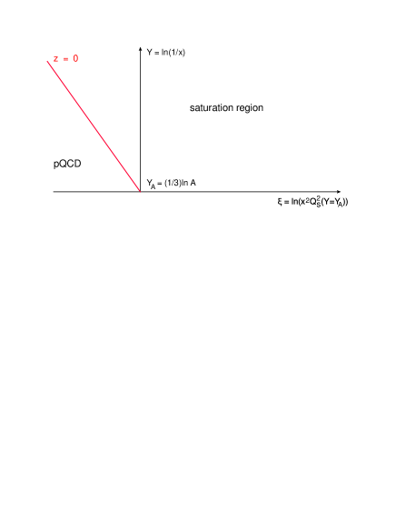
Figure 1: Saturation region of QCD. Red line shows the saturation boundary (z=0).

Indeed, at $Y=Y_{A}$ for DIS with nuclei we have McLerran-Venugopalan formula for the imaginary part of the dipole-nucleus amplitude, which takes the following form (see Fig. 1)

$$N\left(x^{2},Y=Y_{A}\right)\,\,\,=\,\,1\,\,\,-\,\,\,\exp\Big{(}-x^{2}\,Q^{2}_{s}\left(Y=Y_{A},b\right)/4\Big{)}\,\,=\,\,1\,\,\,-\,\,\exp\left(-e^{\xi}\right)$$ (1.8)

One can see that Eq. (1.8) does not reproduce the solution of Eq. (1.7) at $Y=Y_{A}$. Comparing Eq. (1.8) and Eq. (1.7) we see that the geometric scaling behaviour cannot be correct in the entire saturation region.

2 Equation and solution in the momentum space

2.1 Equation and geometric scaling solution

We re-write the Balitsky-Kovchegov equation of Eq. (1.1) in the momentum space introducing

$$N\left(x^{2},b;Y\right)\,\,=\,\,x^{2}\,\int\frac{d^{2}k_{\perp}}{2\pi}\,e^{i\vec{k}_{\perp}\cdot\vec{x}}\,\widetilde{N}\left(k_{\perp},b;Y\right)$$ (2.9)

It takes the form[1, 19]

$$\frac{\partial\widetilde{N}\left(k_{\perp},b;Y\right)}{\partial Y}\,\,=\,\,\bar{\alpha}_{S}\Bigg{\{}\chi\left(-\,\frac{\partial}{\partial\tilde{\xi}}\right)\widetilde{N}\left(k_{\perp},b;Y\right)\,\,\,-\,\,\widetilde{N}^{2}\left(k_{\perp},b;Y\right)\Bigg{\}}$$ (2.10)

where

$$\tilde{\xi}\,\,=\,\,\,\,\ln\left(k^{2}_{\perp}/Q^{2}_{s}\left(Y=Y_{A},b\right)\right)~{}~{}~{}\mbox{and}~{}~{}~{}\tilde{z}\,\,=\,\,\bar{\alpha}_{S}\kappa\left(Y-Y_{A}\right)\,\,-\,\,\tilde{\xi}\,\,=\,\,\ln\left(Q^{2}_{s}\left(Y,b\right)/k^{2}_{\perp}\right)$$ (2.11)

The advantage of the non-linear equation in Eq. (2.10) that the non-linear term depends only on external variable and does not contain the integration over momenta. The BFKL kernel: $\chi\left(-\,\frac{\partial}{\partial\tilde{\xi}}\right)$, can be written as the series over positive powers of $\partial/\partial\tilde{\xi}$ except of the first term

$$\frac{1}{\gamma}\,\widetilde{N}\left(k_{\perp},b;Y\right)\,\,\,\to\,\,\,\int^{k^{2}_{\perp}}\frac{dk^{\prime 2}_{\perp}}{k^{\prime 2}_{\perp}}\widetilde{N}\left(k^{\prime}_{\perp},b;Y\right)$$ (2.12)

Differentiating Eq. (2.10) over $\tilde{\xi}$ one can see that it can be re-written as

$$\frac{\partial\widetilde{N}^{\prime}_{\tilde{\xi}}\left(k_{\perp},b;Y\right)}{\partial Y}\,\,\,=$$ (2.13)

$$\,\,\,\bar{\alpha}_{S}\Bigg{\{}\Big{(}\chi\left(\gamma\right)\,\,-\frac{1}{\gamma}\Big{)}\widetilde{N}^{\prime}_{\tilde{\xi}}\left(k_{\perp},b;Y\right)\,\,+\,\,\widetilde{N}\left(k_{\perp},b;Y\right)\,\,-\,\,2\widetilde{N}^{\prime}_{\tilde{\xi}}\left(k_{\perp},b;Y\right)\widetilde{N}\left(k_{\perp},b;Y\right)\Bigg{\}}$$

where $\gamma\,=\,-\,\frac{\partial}{\partial\tilde{\xi}}$.

Introducing the variable $\tilde{z}$ instead of $\tilde{\xi}$ and the new function $M$ as

$$\widetilde{N}^{\prime}_{\tilde{z}}\left(\tilde{z},b;Y\right)\,\,=\,\,\frac{1}{2}+M\left(\tilde{z},b;Y\right)~{}~{}~{}~{}\mbox{or}~{}~{}~{}~{}\widetilde{N}\left(\tilde{z},b;Y\right)\,\,=\,\,\frac{1}{2}\tilde{z}\,\,+\,\,\int^{\tilde{z}}_{0}d\tilde{z}^{\prime}M\left(\tilde{z}^{\prime},b;Y\right)$$ (2.14)

we can re-write Eq. (2.13) in the form

$$\kappa\,\frac{\partial M\left(\tilde{z},b;Y\right)}{\partial\tilde{z}}\,\,+\,\,\frac{\partial M\left(\tilde{z},b;Y\right)}{\partial Y}\,\,\,=$$ (2.15)

$$\bar{\alpha}_{S}\Bigg{\{}\Big{(}\chi\left(\gamma\right)\,\,-\,\,\frac{1}{\gamma}\Big{)}M\left(\tilde{z},b;Y\right)\,\,-\,\,\,\tilde{z}\,M\left(\tilde{z},b;Y\right)\,\,-\,\,M\left(\tilde{z},b;Y\right)\int^{\tilde{z}}_{0}d\tilde{z}^{\prime}M\left(\tilde{z}^{\prime},b;Y\right)\Bigg{\}}$$

with $\gamma=\frac{\partial}{\partial\tilde{z}}$.

We are going to find solution inside the saturation region where function $M$ is small at large $\tilde{z}$. However, we need to re-write Eq. (2.15) replacing it by

$$\kappa\,\frac{\partial M\left(\tilde{z},b;Y\right)}{\partial\tilde{z}}\,\,+\,\,\frac{\partial M\left(\tilde{z},b;Y\right)}{\partial Y}\,\,\,=$$ (2.16)

$$\bar{\alpha}_{S}\Bigg{\{}\Big{(}\chi\left(\gamma\right)\,\,-\,\,\frac{1}{\gamma}\Big{)}M\left(\tilde{z},b;Y\right)\,\,-\,\,\,\left(\tilde{z}\,+\,\lambda\right)\,M\left(\tilde{z},b;Y\right)\,\,+\,\,M\left(\tilde{z},b;Y\right)\int^{\infty}_{\tilde{z}}d\tilde{z}^{\prime}M\left(\tilde{z}^{\prime},b;Y\right)\Bigg{\}}$$

where

$$\lambda\,\,=\,\,\int^{\infty}_{0}\,d\tilde{z}^{\prime}M\left(\tilde{z}^{\prime},b;Y\right)$$ (2.17)

and neglecting the last term in this equation one can see that we need to solve the following linear equation

$$\kappa\,\frac{\partial M\left(\tilde{z},b;Y\right)}{\partial\tilde{z}}\,\,+\,\,\frac{\partial M\left(\bar{z},b;Y\right)}{\partial Y}\,\,\,=\ \bar{\alpha}_{S}\Bigg{\{}\Big{(}\chi\left(\gamma\right)\,\,-\,\,\frac{1}{\gamma}\Big{)}M\left(\bar{z},b;Y\right)\,\,-\,\,\,\bar{z}\,M\left(\tilde{z},b;Y\right)\,\,\Bigg{\}}$$ (2.18)

with $\gamma\,\,=\,\,\frac{\partial}{\partial\bar{z}}\,\,\mbox{and}\,\,\,\bar{z}\,\,=\,\,\tilde{z}\,+\,\lambda$

First we find the geometrical scaling solution which depends only on $\tilde{z}$. In this case Eq. (2.18) takes the form

$$\kappa\frac{dM\left(\bar{z},b\right)}{d\bar{z}}\,\,\,=\,\,\,\Big{(}\chi\left(\,\gamma\right)\,\,-\,\,\frac{1}{\gamma}\Big{)}M\left(\bar{z},b\right)\,\,-\,\,\,\bar{z}\,M\left(\bar{z},b\right)$$ (2.19)

The boundary condition for this equation we take

$$N^{\prime}_{\tilde{z}}\left(\tilde{z}\,=\,0,b\right)\,\,=\,\,\frac{1}{2}+M\left(\tilde{z}\,=\,0,b\right)\,\,=\,\,\phi_{0}(b)\,\,\ll\,\,1$$ (2.20)

where $\phi_{0}(b)$ is the solution to the linear BFKL equation at $\tilde{z}=0$. $\phi_{0}(b)\,\leq\,1$ due to unitarity constraint and should be small to neglect that non-liner term at $\tilde{z}=0$.

Eq. (2.19) can be solved using the Mellin transform

$$M\left(\tilde{z},b\right)=\int^{\epsilon+i\infty}_{\epsilon-i\infty}\frac{d\gamma}{2\pi i}e^{\gamma\,\bar{z}}m\left(\gamma,b\right)$$ (2.21)

where $m\left(\gamma,b\right)$ satisfies the equation:

$$\left(\kappa\gamma-\chi\left(\gamma\right)+1/\gamma\right)\,m\left(\gamma,b\right)=\frac{dm\left(\gamma,b\right)}{d\gamma}.$$ (2.22)

The solution for $m\left(\gamma,b\right)$ takes the following form

$$m\left(\gamma\right)\,\,=\,\,\exp\Bigg{(}\int^{\gamma}_{0}d\gamma^{\prime}\Big{(}\kappa\gamma^{\prime}-\chi\left(\gamma^{\prime}\right)+1/\gamma^{\prime}\Big{)}\Bigg{)}$$ (2.23)

and taking into account the explicit form of the BFKL kernel given by Eq. (1.4) one can re-write Eq. (2.23) in the form

$$m\left(\gamma\right)\,\,=\,\,\exp\Bigg{(}\kappa\gamma^{2}/2-2\psi(1)\gamma\Bigg{)}\,\Bigg{(}\frac{\gamma\Gamma(\gamma)}{\Gamma(1-\gamma)}\Bigg{)}\,\,=\,\,\exp\Bigg{(}\kappa\gamma^{2}/2-2\psi(1)\gamma\Bigg{)}\,\frac{\Gamma(1+\gamma)}{\Gamma(1-\gamma)}$$ (2.24)

Substituting Eq. (2.24) into Eq. (2.21) we obtain

$$M\left(\bar{z},b\right)=\int^{\epsilon+i\infty}_{\epsilon-i\infty}\frac{d\gamma}{2\pi i}e^{\gamma\bar{z}\,+\,\kappa\gamma^{2}/2}\,\frac{\Gamma(1+\gamma)}{\Gamma(1-\gamma)}$$ (2.25)

where for $\bar{z}$ we use a new definition: $\bar{z}\,\,=\,\,\tilde{z}\,+\,\lambda\,\,-2\,\,\psi\left(1\right)$.

One can see that in Eq. (2.25) we cannot close the contour of integration in $\gamma$ neither on the left semi-plane nor on the right one. Introducing $\gamma\,=\,i\,\bar{\gamma}$ we reduce Eq. (2.25) to the form

$$M\left(\bar{z},b\right)=\int^{+\infty}_{-\infty}\frac{d\bar{\gamma}}{2\pi}e^{i\,\bar{\gamma}\bar{z}\,-\,\kappa\bar{\gamma}^{2}/2}\,\frac{\Gamma(1+i\bar{\gamma})}{\Gamma(1-i\bar{\gamma})}$$ (2.26)

For large $\tilde{z}$ and $\bar{\gamma}$ is large about $\tilde{z}$, we can use the approximation

$$\Gamma\left(1+i\bar{\gamma}\right)\,\,\xrightarrow{\bar{\gamma}\,\gg\,1}\,\,\sqrt{2\pi}|\bar{\gamma}|^{\frac{1}{2}}\,e^{-\frac{1}{2}\pi|\bar{\gamma}|}$$ (2.27)

(see formula 8.328 of Ref.[20]). Using Eq. (2.27), Eq. (2.26) takes the form

$$M\left(\bar{z},b\right)\,\,=\,\,\int^{+\infty}_{-\infty}\frac{d\bar{\gamma}}{2\pi}e^{i\,\bar{\gamma}\bar{z}\,-\,\kappa\bar{\gamma}^{2}/2\,}$$ (2.28)

which is equal (see formulae 3.462(3), 9.246 of Ref. [20])

$$M\left(\bar{z},b\right)\,\,=\,\,\frac{1}{\sqrt{2\pi\kappa}}\,e^{-\frac{\bar{z}^{2}}{4\kappa}}\,D_{0}\left(-\frac{\bar{z}}{\sqrt{\kappa}}\right)\,\,\,=\,\,\frac{1}{\sqrt{2\pi\kappa}}\,e^{-\frac{\bar{z}^{2}}{2\kappa}}$$ (2.29)

where $D_{n}(z)=2^{-\frac{1}{2}n}e^{-\frac{\bar{z}^{2}}{4}}H_{n}(z/\sqrt{2})$ is the parabolic cylinder function (see formulae 9.24 - 9.25 of Ref.[20]).

Therefore we reproduce the solution of Eq. (1.7). Choosing the coefficient in front of Eq. (2.29) we can easily satisfy the initial condition of Eq. (2.20) which leads to the solution

$$M\left(\bar{z},b\right)\,\,=\,\,\left(\phi_{0}\left(b\right)-\frac{1}{2}\right)\,e^{-\frac{\bar{z}^{2}}{2\kappa}}$$ (2.30)

2.2 General solution and initial condition at $Y=Y_{A}$

As has been mentioned we are not able to find the geometric scaling solution that satisfy both initial and boundary conditions given by Eq. (1.8) and Eq. (2.20). We need to solve a general Eq. (2.18) to find such a solution. We start with re-writing boundary condition of Eq. (1.8) for function $M\left(\tilde{z},b;Y\right)$ in momentum representation.

$$\frac{1}{2}\,\,+\,M\left(\tilde{z},b;Y=Y_{A}\right)\,\, = \,\,\frac{d}{d\tilde{z}}\int\frac{d^{2}r}{r^{2}}\,e^{i\vec{k}\cdot\vec{r}}\,\Big{(}1\,-\,\exp\left(-r^{2}\,Q^{2}_{s}\left(b;Y=Y_{A}\right)/4\right)\Big{)}\,\,$$

$$= \,\,\frac{d}{d\tilde{z}}\left(\frac{1}{2}\Gamma_{0}\left(\frac{k^{2}_{\perp}}{Q^{2}_{s}\left(b;Y=Y_{A}\right)}\right)\right)\,\,=\frac{d}{d\tilde{z}}\left(\frac{1}{2}\Gamma_{0}\left(e^{-\,\tilde{z}}\right)\right)\,\,=\,\,\frac{1}{2}\exp\Big{(}-\,e^{-\,\tilde{z}}\Big{)}$$

$$M\left(z,b;Y=Y_{A}\right) = -\frac{1}{2}\left(1\,\,-\,\,\exp\Big{(}-e^{-\,\tilde{z}}\Big{)}\right)$$ (2.31)

We solve Eq. (2.18) using the double Mellin transform: viz.

$$M\left(\tilde{z},b;Y\right)\,\,=\,\,\int^{\epsilon+i\infty}_{\epsilon-i\infty}\frac{d\omega}{2\pi i}\int^{\epsilon+i\infty}_{\epsilon-i\infty}\frac{d\gamma}{2\pi i}e^{\omega\left(Y-Y_{A}\right)+\gamma\tilde{z}}\,m\left(\omega,\gamma;b\right)$$ (2.32)

For $m\left(\omega,\gamma;b\right)$ the equation takes the form

$$\left(\omega\,+\,\kappa\gamma\,-\,\chi\left(\gamma\right)\,+\,\frac{1}{\gamma}\right)m\left(\omega,\gamma\right)\,=\,\frac{\partial m\left(\omega,\gamma\right)}{\partial\gamma}$$ (2.33)

Solution to Eq. (2.33) can be written in the form

$$M\left(\bar{z},Y\right) = \int^{\epsilon+i\infty}_{\epsilon-i\infty}\!\!\frac{d\omega}{2\pi i}e^{\omega\left(Y-Y_{A}\right)}\int^{\epsilon+i\infty}_{\epsilon-i\infty}\!\!\frac{d\gamma}{2\pi i}I\left(\omega\right)\exp\Bigg{(}\omega\,\gamma\,\,+\,\,\gamma\bar{z}+\kappa\gamma^{2}/2\Bigg{)}\frac{\Gamma(1+\gamma)}{\Gamma(1-\gamma)}$$ (2.34)

where function $I\left(\omega\right)$ has to be found from Eq. (2.2). At $Y=Y_{A}$ Eq. (2.2) can be written as

$$M\left(Y=Y_{A},\bar{z}\right)\,=$$

$$\,\int^{\epsilon+i\infty}_{\epsilon-i\infty}\!\!\frac{d\omega}{2\pi i}\int^{\epsilon+i\infty}_{\epsilon-i\infty}\!\!\frac{d\gamma}{2\pi i}I\left(\omega\right)\exp\Bigg{(}\omega\,\gamma\,\,+\,\,\gamma\bar{z}+\kappa\gamma^{2}/2\Bigg{)}\frac{\Gamma(1+\gamma)}{\Gamma(1-\gamma)}$$

$$=\,\int^{\epsilon+i\infty}_{\epsilon-i\infty}\!\!\frac{d\gamma}{2\pi i}J\left(\gamma\right)\exp\Bigg{(}\gamma z+\kappa\gamma^{2}/2\,+\,2\psi(1)\gamma\Bigg{)}\frac{\Gamma(1+\gamma)}{\Gamma(1-\gamma)}$$ (2.35)

One can see that

$$J\left(\gamma\right)\,\,=\int^{\epsilon+i\infty}_{\epsilon-i\infty}\!\!\frac{d\omega}{2\pi i}\,e^{\omega\,\gamma}\,I\left(\omega\right)\,=\,\frac{1}{2}\,\frac{\Gamma\left(1-\gamma\right)}{\Gamma\left(1+\gamma\right)}\,\left(\Gamma\left(\gamma\right)\,\,-\,\,\frac{1}{\gamma}\right)\,\exp\left(-\frac{\kappa\gamma^{2}}{2}\right)$$ (2.36)

leads to Eq. (2.2). Indeed, substituting Eq. (2.36) into Eq. (2.2) one obtains Eq. (2.2) closing contour in $\gamma$ over negative $\gamma$-s

For $Y>Y_{A}$ the solution takes the form

$$M\left(Y,\bar{z}\right)\,\,=\,\,\int^{\epsilon+i\infty}_{\epsilon-i\infty}\!\!\frac{d\gamma}{2\pi i}J\left(Y\,\,+\,\gamma\right)\exp\Bigg{(}\gamma\bar{z}+\kappa\gamma^{2}/2\Bigg{)}\frac{\Gamma(1+\gamma)}{\Gamma(1-\gamma)}$$ (2.37)

$$=\,\,\,\frac{1}{2}\int^{\epsilon+i\infty}_{\epsilon-i\infty}\!\!\frac{d\gamma}{2\pi i}\exp\Big{(}\gamma\bar{z}-\frac{1}{2}\kappa Y^{2}-\kappa Y\gamma\Big{)}\,\frac{\Gamma\left(1+\gamma\right)}{\Gamma\left(1-\gamma\right)}\,\frac{\Gamma\left(1-\gamma-Y\right)}{\Gamma\left(1+\gamma+Y\right)}\,\left(\Gamma\left(\gamma+Y\right)\,\,-\,\,\frac{1}{\gamma+Y}\right)$$

$$=\,\,\,\frac{1}{2}e^{-\frac{1}{2}\kappa Y^{2}}\int^{\epsilon+i\infty}_{\epsilon-i\infty}\!\!\frac{d\gamma}{2\pi i}\exp\Big{(}-\gamma\tilde{\xi}\,+\,2\,\psi(1)\,Y\Big{)}\,\frac{\Gamma\left(1+\gamma\right)}{\Gamma\left(1-\gamma\right)}\frac{\Gamma\left(1-\gamma-Y\right)}{\Gamma\left(1+\gamma+Y\right)}\,\left(\Gamma\left(\gamma+Y\right)\,\,-\,\,\frac{1}{\gamma+Y}\right)$$

$$=\,\,\,-\frac{1}{2}e^{-\frac{1}{2}\kappa Y^{2}}\int^{\epsilon+i\infty}_{\epsilon-i\infty}\!\!\frac{d\gamma}{2\pi i}\exp\Big{(}-\gamma\tilde{\xi}\,+\,2\,\psi(1)\,Y\Big{)}\,\frac{\Gamma\left(1+\gamma\right)}{\Gamma\left(1-\gamma\right)}\frac{\Gamma\left(-\gamma-Y\right)}{\Gamma\left(\gamma+Y\right)}\,\left(\Gamma\left(\gamma+Y\right)\,\,-\,\,\frac{1}{\gamma+Y}\right)$$

$$=\,\,\,-\frac{1}{2}\,e^{-\frac{1}{2}\kappa Y^{2}\,\,\,+\,2\,\psi(1)\,Y}\,\Bigg{\{}\,I_{1}\left(Y,\tilde{\xi}\right)\,\,-\,\,I_{2}\left(Y,\tilde{\xi}\right)\,\Bigg{\}}$$

Since $\tilde{\xi}\,\,<\,\,0$ we can take the integrals over $\gamma$ in $I_{1}\left(Y,\tilde{\xi}\right)$ and in $I_{2}\left(Y,\tilde{\xi}\right)$ closing contours of integrations on the left semi-plane. In $I_{1}\left(\tilde{\xi}\right)$ and $I_{2}\left(\tilde{\xi}\right)$ we have two sets of poles: $\gamma\,=\,-n-1$ from $\Gamma\left(1+\gamma\right)$ and $\gamma\,\,=\,\,n-[Y]$ where $[Y]$ is the integer part or floor function of $Y$, from $\Gamma\left(-\gamma-Y\right)$. These sets lead to the following contributions to $I_{1}\left(Y,\tilde{\xi}\right)$ and to $I_{2}\left(Y,\tilde{\xi}\right)$:

$$I_{1}\left(Y,\tilde{\xi}\right)\,\,\, = \,\,\,I^{1}_{1}\left(Y,\tilde{\xi}\right)\,\,+\,\,I^{2}_{1}\left(Y,\tilde{\xi}\right)\,;$$

$$I^{1}_{1}\left(Y,\tilde{\xi}\right)\,\,\, = \,\,\,\sum^{\infty}_{n=0}\frac{(-1)^{n}}{n!}\frac{\Gamma\left(n+1-Y\right)}{\Gamma\left(n+2\right)}\,e^{(n+1)\tilde{\xi}}\,\,=\,\,e^{\tilde{\xi}}\,\Gamma\left(1-Y\right)\,{}_{1}F_{1}\left(1-Y,2,-e^{\tilde{\xi}}\right)\,;$$ (2.38)

$$I^{2}_{1}\left(Y,\tilde{\xi}\right)\,\,\, = \,\,e^{\tilde{\xi}\,Y}\,\sum^{[Y]}_{n=0}\frac{(-1)^{n}}{n!}\frac{\Gamma\left(n+1-Y\right)}{\Gamma\left(1-n+Y\right)}\,e^{-n\,\tilde{\xi}}\,;$$ (2.39)

$$I_{2}\left(Y,\tilde{\xi}\right)\,\,\, = \,\,\,I^{1}_{2}\left(Y,\tilde{\xi}\right)\,\,+\,\,I^{2}_{2}\left(Y,\tilde{\xi}\right)\,;$$

$$I^{1}_{2}\left(Y,\tilde{\xi}\right)\,\,\, = \,\,\,\sum^{\infty}_{n=0}\frac{(-1)^{n}}{n!}\frac{\Gamma\left(n+1-Y\right)}{\Gamma\left(n+2\right)\,\Gamma\left(Y-n\right)}\,e^{(n+1)\tilde{\xi}}\,\,=\,\,e^{\tilde{\xi}}\,\frac{\Gamma\left(1-Y\right)}{\Gamma\left(Y\right)}\,{}_{2}F_{1}\left(1-Y,-Y,2,-e^{\tilde{\xi}}\right)\,;$$ (2.40)

$$I^{2}_{2}\left(Y,\tilde{\xi}\right)\,\,\, = \,\,e^{\tilde{\xi}\,Y}\,\sum^{[Y]}_{n=0}\frac{(-1)^{n}}{n!}\frac{\Gamma\left(n+1-Y\right)}{\Gamma\left(1-n+Y\right)\,\Gamma\left(n+1\right)}\,e^{-\,n\,\tilde{\xi}}\,;$$ (2.41)

In Eq. (2.38) - Eq. (2.41) ${}_{1}F_{1}\left(\alpha,\beta,t\right)$ is the confluent hypergeometric function (another notation is $\Phi\left(\alpha,\beta,t\right)$, see formulae 9.2 of Ref. [20]) and ${}_{2}F_{1}\left(\alpha,\beta,\gamma,t\right)$ is the hypergeometric function (see formulae 9.1 of Ref. [20]).

For matching of this solution with the solution given by Eq. (2.30) we need to know the asymptotic behaviour of Eq. (2.38)-Eq. (2.41) at large values of $Y$. Using Kummer’s transformation: ${}_{1}F_{1}\left(\alpha,\beta,t\right)\,\,=\,\,e^{t}\,{}_{1}F_{1}\left(\beta-\alpha,\beta,-t\right)$ we can re-write Eq. (2.38) in the form

$$I^{1}_{1}\left(Y,\tilde{\xi}\right)\,\,\, = \,\,e^{\tilde{\xi}}\,\Gamma\left(1-Y\right)\exp\left(-e^{\tilde{\xi}}\right)\,{}_{1}F_{1}\left(1+Y,2,e^{\tilde{\xi}}\right)\,\,$$

$$\xrightarrow{Y\,\gg\,1} \,\,e^{\tilde{\xi}}\exp\left(-e^{\tilde{\xi}}\right)\,\Gamma\left(1-Y\right)\sum^{\infty}_{n=0}\frac{Y^{n}}{n!(n+1)!}e^{n\tilde{\xi}}\,=\,e^{\tilde{\xi}}\exp\left(-e^{\tilde{\xi}}\right)\frac{\Gamma\left(1-Y\right)}{2\sqrt{Y\,e^{\tilde{\xi}}}}I_{1}\left(2\sqrt{Y\,e^{\tilde{\xi}}}\right)$$

where $I_{1}\left(t\right)$ is the modified Bessel function of the first kind (see formulae 8.445 - 8.451 of Ref.[20]). Using their asymptotic behaviour at large values of the argument we obtain

$$I^{1}_{1}\left(Y,\tilde{\xi}\right)\,\,\xrightarrow{Y\gg 1}\,\,e^{\tilde{\xi}}\exp\left(-e^{\tilde{\xi}}\right)\,e^{-\,Y\left(\ln Y-1\right)}\frac{1}{\sqrt{2\pi\left(4Y\exp\left(\tilde{\xi}\right)\right)^{3}}}\,\exp\left(2\sqrt{Y\exp\left(\tilde{\xi}\right)}\right)$$ (2.43)

We replace Eq. (2.39) by the integral, i.e.

$$I^{2}_{1}\left(Y,\tilde{\xi}\right)\,\,\to\,\,e^{\tilde{\xi}\,Y}\int^{Y}_{0}dt\frac{\Gamma\left(1+t-Y\right)}{\Gamma\left(1-t+Y\right)\,\Gamma\left(1+t\right)}\,\,e^{-\tilde{\xi}\,t\,+\,i\,\pi\,t}$$ (2.44)

The steepest decent method leads to the following contribution

$$I^{2}_{1}\left(Y,\tilde{\xi}\right)\,\,\to\,\,\,\sqrt{\pi\left(Y\,e^{\tilde{\xi}}\right)^{\frac{1}{2}}}e^{-Y\ln Y}$$ (2.45)

at the saddle point $t_{SP}$ which can be found from the equation

$$-\ln t_{SP}+2\ln\left(Y-t_{SP}-1\right)\,-\,\tilde{\xi}\,=\,0\,;\,\,\,\,\,\,\,\,\,\,\,\,\,t_{SP}\,=\,Y-\sqrt{Y}e^{\frac{1}{2}\,\tilde{\xi}}\,\,\,\,\,\mbox{at}\,\,\,\,Y\,\gg\,1$$ (2.46)

The large $Y$ behaviour of Eq. (2.40) can be obtained using the transformation ${}_{2}F_{1}(\alpha,\beta,\gamma,t)=(1-t)^{\gamma-\alpha-\beta}{}_{2}F_{1}(\gamma-\alpha,\gamma-\beta,\gamma,t)$ (see formulae 9.131 of Ref. [20])

$$\begin{array}[]{rcl}I^{1}_{2}(Y,\tilde{\xi})&=&e^{\tilde{\xi}}\frac{\Gamma(1-Y)}{\Gamma(Y)}{}_{2}F_{1}(1-Y,-Y,2,-e^{\tilde{\xi}})=(1+e^{\tilde{\xi}})^{1+2y}{}_{2}F_{1}(1+y,2+y,2,-e^{\tilde{\xi}})\\ \\ &\xrightarrow{Y\,\gg\,1}&\sum^{\infty}_{n=0}\frac{(\Gamma(Y+n))^{2}}{(\Gamma(Y))^{2}}\frac{(-e^{\tilde{\xi}})^{n}}{n!(n+1)!}=e^{\tilde{\xi}}e^{-2Y(\ln Y-1)}\frac{1}{2Ye^{\frac{1}{2}\tilde{\xi}}}J_{1}(2Ye^{\frac{1}{2}\tilde{\xi}})\end{array}$$

and knowing the asymptotic representation of Bessel function we get

$$\begin{array}[]{rcr}I^{1}_{2}(Y,\tilde{\xi})&\xrightarrow{Y\,\gg\,1}&\frac{1}{2}e^{\tilde{\xi}}e^{-2Y(\ln Y-1)}\frac{1}{(Ye^{\frac{1}{2}\tilde{\xi}})^{\frac{3}{2}}}\left\{\cos(\{8Ye^{\frac{\tilde{\xi}}{2}}-3\pi\}/4)\left[\frac{\Gamma(7/2)}{\Gamma(-1/2)}+O((y^{2}e^{\tilde{\xi}})^{-1})\right]\right.\\ \\ &&\left.-\sin(\{8Ye^{\frac{\tilde{\xi}}{2}}-3\pi\}/4)\left[\frac{\Gamma(9/2)}{\Gamma(-3/2)}+O((y^{2}e^{\tilde{\xi}})^{-1})\right]\right\}\end{array}$$ (2.47)

Finally, we replace Eq. (2.41) by the integral to estimate the large $Y$ dependence of this term, i.e.

$$I^{2}_{2}\left(Y,\tilde{\xi}\right)\,\,\to\,\,e^{\tilde{\xi}\,Y}\int^{Y}_{0}dt\,\frac{\Gamma\left(1+t-Y\right)}{\Gamma\left(1-t+Y\right)\,\Gamma^{2}\left(1+t\right)}\,\,e^{-\tilde{\xi}\,t\,+\,i\,\pi\,t}$$ (2.48)

Taking the integral by the steepest decent method in the same way as in Eq. (2.47) we obtain the equation for the saddle point $t_{SP}$:

$$-2\ln t_{SP}+2\ln\left(Y-t_{SP}-1\right)\,-\,\tilde{\xi}\,=\,0\,;\,\,\,\,\,\,\,\,\,\,\,\,\,t_{SP}\,=\,\frac{Y-1}{1+e^{\frac{1}{2}\tilde{\xi}}}$$ (2.49)

and

$$I^{2}_{2}\left(Y,\tilde{\xi}\right)\,\,\to\,\,\,\sqrt{\frac{\pi(Y-1)e^{\frac{1}{2}\tilde{\xi}}}{4\left(1-e^{\tilde{\xi}}\right)}}\,e^{-2Y\ln Y+Y\tilde{\xi}\frac{e^{\frac{1}{2}\tilde{\xi}}}{1+e^{\frac{1}{2}\tilde{\xi}}}}$$ (2.50)

Comparing Eq. (2.43), Eq. (2.45), Eq. (2.47) and Eq. (2.50) we see that at large values of $Y$ solutions of Eq. (2.30) and of Eq. (2.37) match each other on the line $\tilde{\xi}\,=\,-\,\ln Y$ which can be translate as the line in $(Y,\tilde{z})$ plane (see Fig. 2):

$$\tilde{z}\,\,=\,\,\bar{\alpha}_{S}\kappa Y\,\,+\,\,\ln Y$$ (2.51)

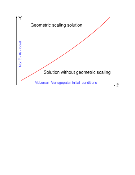
Figure 2: Saturation region: two domains in which there is the geometric scaling behaviour of the solution and there is no such behaviour. The border red line is Eq. (2.51).

3 Matching two solutions: at small $\tilde{z}$ and at large $\tilde{z}$

3.1 Corrections at large $\tilde{z}$

In this section we are going to find the first correction to the non-linear equation (see Eq. (2.16)) deeply in the saturation region where we expect that solution has a geometric scaling behaviour, or in other words, it is a function of $\tilde{z}$. One can see that the equation for first correction takes the following form after substituting $M\,\,=\,\,M^{(0)}+M^{(1)}$ into Eq. (2.16):

$$\kappa\frac{dM^{(1)}\left(\bar{z}\right)}{d\tilde{z}}=\Big{\{}\chi\left(\gamma\right)\,-\,\frac{1}{\gamma}\Big{\}}M^{(1)}\left(\tilde{z}\right)\,\,-\,\,\bar{z}M^{(1)}\left(\bar{z}\right)\,\,+\,\,M^{(0)}\left(\bar{z}\right)\int^{\infty}_{\bar{z}}dz^{\prime}M^{(0)}\left(z^{\prime},Y\right)$$ (3.52)

where $\lambda=\int^{\infty}_{0}M^{(0)}\left(z^{\prime}\right)dz^{\prime}\,\,=\,\,A\sqrt{\frac{\pi\kappa}{2}}$.

In Eq. (3.52) $M^{(0)}$ is the solutions to Eq. (2.19) that takes the form

$$M^{(0)}\left(\bar{z}\right)\,\,=\,\,A\,\exp\left(-\bar{z}^{2}/\left(2\kappa\right)\right)$$ (3.53)

which we will use below. It should be noted that $A\,<\,0$ due to unitarity constraints; and Eq. (2.30) for $A$ was derived from the matching of this solution at $\tilde{z}=0$. Here, we wish to suggest a better procedure for matching.

Using Eq. (3.53) we can re-write the equation for the first correction as follows

$$\kappa\frac{dM^{(1)}\left(\bar{z}\right)}{d\bar{z}}\,\,=\,\,\Big{\{}\chi\left(\gamma\right)\,-\,\frac{1}{\gamma}\Big{\}}M^{(1)}\left(\bar{z}\right)\,\,-\,\,\bar{z}M^{(1)}\left(\bar{z}\right)\,\,+\,\,M^{(0)}\left(\bar{z}\right)\int^{\infty}_{\bar{z}}dz^{\prime}M^{(0)}\left(z^{\prime},Y\right)$$ (3.54)

After taking the integral the last term of this equation can be reduced to the form

$$M^{(0)}\left(\bar{z}\right)\int^{\infty}_{\bar{z}}dz^{\prime}M^{(0)}\left(z^{\prime},Y\right)\,\,=\,\,M^{(0)}\left(\bar{z}\right)\,A\,\sqrt{\frac{\pi\kappa}{2}}\,\mbox{Erfc}\left(\frac{\bar{z}}{\sqrt{2\kappa}}\right)\,\,\xrightarrow{z\gg 1}\,\,A^{2}\,\frac{\kappa}{\bar{z}}\,e^{-\frac{\bar{z}^{2}}{\kappa}}$$ (3.55)

Using the Mellin transform of Eq. (2.21) we obtain Eq. (3.54) in the form:

$$\left(\kappa\,\gamma\,-\chi\left(\gamma\right)+\frac{1}{\gamma}\,+\,\lambda\right)m^{(1)}\left(\gamma\right)\,\,=\,\,\frac{dm^{(1)}\left(\gamma\right)}{d\gamma}\,\,+\,\,2\,A^{2}\frac{\sqrt{\pi\kappa}}{\gamma}\,e^{\kappa\gamma^{2}/4}.$$ (3.56)

The solution to Eq. (3.56) takes the form (see Ref.[21])

$$m^{(1)}\left(\gamma\right)\,\,=\,\,m^{(0)}\left(\gamma\right)\,A^{2}\,\int^{\infty}_{\gamma}\frac{d\gamma^{\prime}}{m^{(0)}\left(\gamma^{\prime}\right)}\frac{\sqrt{\pi\kappa}}{\gamma^{\prime}}\,e^{\kappa\gamma^{\prime 2}/4}\,\,=\,\,m^{(0)}\left(\gamma\right)\,A^{2}\,\sqrt{\pi\kappa}\,\int^{\infty}_{\gamma}\frac{d\gamma^{\prime}}{\gamma^{\prime}}\frac{\Gamma\left(1-\gamma^{\prime}\right)}{\Gamma\left(1+\gamma^{\prime}\right)}\,e^{-\kappa\gamma^{\prime 2}/4}$$ (3.57)

where $m^{(0)}$ is given by Eq. (2.24). As has been discussed in the integral of Eq. (2.21) we expect that large $\gamma$’s will be essential. In Eq. (3.57) the typical $d\gamma^{\prime}\sim 1/\sqrt{\kappa}\,\ll\,\gamma$ and we can replace this integral by

$$m^{(1)}\left(\gamma\right)=2m^{(0)}\left(\gamma\right)\,A^{2}\,\sqrt{\pi\kappa}\,\frac{\Gamma\left(1-\gamma\right)}{\Gamma\left(1+\gamma\right)}\int^{\infty}_{\gamma}\frac{d\gamma^{\prime}}{\gamma^{\prime}}\,e^{-\kappa\gamma^{\prime 2}/4}=-\,2\,m^{(0)}\left(\gamma\right)\,A^{2}\,\sqrt{\pi\kappa}\,\frac{\Gamma\left(1-\gamma\right)}{\Gamma\left(1+\gamma\right)}\,Ei\left(-\kappa\gamma^{2}/4\right)$$ (3.58)

See Ref.[20]: formula 3.352(2) for the last integration and formula 8.21 for the exponential integral $E\left(x\right)$. For large $\gamma$ Eq. (3.58) takes the form

$$m^{(1)}\left(\gamma\right)\,\,=\,\,\,m^{(0)}\left(\gamma\right)\,A^{2}\,\sqrt{\pi\kappa}\,\,\frac{\Gamma\left(1-\gamma\right)}{\Gamma\left(1+\gamma\right)}\,\,\frac{4}{\kappa\gamma^{2}}\exp\Big{(}-\kappa\gamma^{2}/4\Big{)}$$ (3.59)

Plugging Eq. (3.59) in Eq. (2.21) we obtain $M^{(1)}\left(\bar{z}\right)$ in the form

$$M^{(1)}\left(\bar{z}\right)\,\,\,=\,\,A^{2}\frac{4\,\sqrt{\pi\kappa}}{\kappa}\,\,\int^{\epsilon+i\infty}_{\epsilon-i\infty}\frac{d\gamma}{2\pi i}\,\frac{1}{\gamma^{2}}\,e^{\gamma\bar{z}\,\,+\,\,\frac{\kappa\gamma^{2}}{4}}\,\,=\,\,-A^{2}e^{-\bar{z}^{2}/2\kappa}\,D_{-2}\left(\bar{z}\sqrt{\frac{2}{\kappa}}\right)\,\,\xrightarrow{\bar{z}\gg 1}\,\,-A^{2}\frac{\kappa}{\bar{z}^{2}}e^{-\bar{z}^{2}/\kappa}$$ (3.60)

where $D_{p}\left(z\right)$ is the parabolic cylinder function (see formulae 9.24 - 9.25 of Ref. [20]).

3.2 Corrections at small $\tilde{z}$

In the region of small $\tilde{z}$ we can solve Eq. (2.10) for the amplitude $N\left(\tilde{z}\right)$ noting that the geometric scaling solution to the BFKL equation occurs at $\gamma=\gamma_{cr}$. In the vicinity of the saturation scale the linear BFKL equation can be simplified and replaced by

$$\frac{d\widetilde{N}\left(\tilde{z}\right)}{d\tilde{z}}\,\,=\,\,\left(1-\gamma_{cr}\right)\,\widetilde{N}\left(\tilde{z}\right)$$ (3.61)

One can see that this equation leads to $\widetilde{N}\left(\tilde{z}\right)\,\,\propto\,\,\exp\left((1-\gamma_{cr})\tilde{z}\right)$. The solution to the BFKL equation with full kernel in the vicinity of the saturation scale takes the form [11, 10, 12]

$$\widetilde{N}\left(\tilde{z};Q_{s}\left(Y\right)\right)\,\,=\,\,\phi_{0}\,e^{\left(1-\gamma_{cr}\right)\tilde{z}}\exp\Bigg{(}-\frac{\tilde{z}^{2}}{2\frac{\chi^{\prime\prime}_{\gamma\gamma}\left(\gamma_{cr}\right)}{\kappa}\,\ln\left(Q^{2}_{s}\left(Y\right)/Q^{2}_{s}\left(0\right)\right)}\Bigg{)}$$ (3.62)

Therefore, we can trust Eq. (3.61) only for

$$\tilde{z}\,~{}~{}\ll\,~{}~{}\sqrt{2\frac{\chi^{\prime\prime}_{\gamma\gamma}\left(\gamma_{cr}\right)}{\kappa}\ln\left(Q^{2}_{s}\left(Y\right)/Q^{2}_{s}\left(0\right)\right)}\,\,\,\,=\,\,\,\,9.9\,\sqrt{Y}$$ (3.63)

For such $\tilde{z}$ the non-linear equation (see Eq. (2.10)) can be re-written in the form

$$\kappa\,\frac{d\widetilde{N}\left(\tilde{z}\right)}{d\tilde{z}}\,\,=\,\,\kappa\left(1-\gamma_{cr}\right)\,\widetilde{N}\left(\tilde{z}\right)\,\,-\,\,\widetilde{N}^{2}\left(\tilde{z}\right)$$ (3.64)

The solution to this equation that satisfies the initial condition $\widetilde{N}\left(\tilde{z}=0\right)=N_{0}$ takes the following form

$$\widetilde{N}\left(\tilde{z}\right)\,\,=\,\,\frac{\kappa\left(1-\gamma_{cr}\right)\,N_{0}}{N_{0}\,\,-\,\,\left(N_{0}\,-\,\kappa\left(1-\gamma_{cr}\right)\right)e^{-\left(1-\gamma_{cr}\right)\,\tilde{z}}}$$ (3.65)

As we will discuss in the next subsection the scattering amplitude in the coordinate space is equal to

$$N\left(z\right)\,\,=\,\,2\frac{d\widetilde{N}\left(z\right)}{dz}\,\,=\,\,-2\,\frac{\kappa\left(1-\gamma_{cr}\right)^{2}\left(N_{0}-\kappa\left(1-\gamma_{cr}\right)\right)\,N_{0}\,e^{-\left(1-\gamma_{cr}\right)\,z}}{\left(N_{0}\,\,-\,\,\left(N_{0}\,-\,\kappa\left(1-\gamma_{cr}\right)\right)e^{-\left(1-\gamma_{cr}\right)\,z}\right)^{2}}$$ (3.66)

We will use this equation in the matching procedure described below in the next section.

3.3 Matching procedure

In this subsection we would like to discuss matching of two solutions at small and large $\tilde{z}$. First, we calculate the scattering amplitude of two dipoles in the coordinate representation where we know that at large $z$ this amplitude $N\left(z\right)\to 1$.

From Eq. (2.9) we see that

$$2\pi\widetilde{N}\left(k_{\bot},b;Y\right)\,\,=\,\,2\,\pi\int xdx\frac{J_{0}\left(k_{\bot}\,x\right)}{x^{2}}N\left(x,b;Y\right)$$ (3.67)

The main contribution to the integral over $x$ stems from $k_{\bot}\,x\leq 2.4$, where 2.4 is the zero of $J_{0}\left(k_{\bot}x\right)$ ($J_{0}\left(k_{\bot}x=2.4\right)=0$), and therefore, we can replace the integral by

$$\widetilde{N}\left(k_{\bot},b;Y\right)\,\,=\,\frac{1}{2}\,\int^{\frac{2.4^{2}}{k^{2}_{\bot}}}_{0}\frac{dx^{2}}{x^{2}}N\left(x,b;Y\right)\,\,=\,\,\frac{1}{2}\int^{\ln\left(2.4^{2}/k^{2}_{\bot}\right)}_{-\infty}d\ln x^{2}N\left(x^{2},b,Y\right)$$ (3.68)

or

$$N\left(x,b,Y\right)\,\,=\,2\,\frac{d\widetilde{N}\left(k_{\bot},b;Y\right)}{d\ln(2.4^{2}/k^{2}_{\bot})}$$ (3.69)

For the solution with the geometric scaling behaviour Eq. (3.69) takes the form

$$N\left(z\right)\,\,=\,\,2\,\frac{d\widetilde{N}\left(\tilde{z}\right)}{d\tilde{z}}$$ (3.70)

Bearing Eq. (3.70) in mind we can formulate the matching procedure in the following way

$$N_{z\,<\,1}\left(z_{m},N_{0}\right)\,\,=\,\,N^{(0)}_{z\,>\,1}\left(z_{m},A\right)\,\,=\,\,1\,+\,2\,M^{(0)}\left(z_{m},A\right)$$

$$\frac{dN^{(0)}_{z\,<\,1}\left(z_{m},A\right)}{dz}\,\,=\,\,+\,2\,\frac{dM^{(0)}\left(z_{m},A\right)}{dz}$$ (3.71)

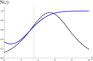
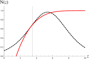
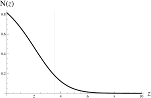
Fig. 3-a	Fig. 3-b	Fig. 3-c
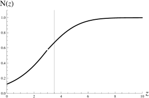
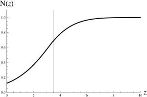
Fig. 3-d	Fig. 3-e	Fig. 3-f

Figure 3: The scattering amplitude $N\left(z\right)$ in the coordinate representation: (Fig. 3-a) matching of two solutions: $N\left(z\right)$ at $z<1$ ( dashed black b line) and $N^{(0)}\left(z\right)z\gg 1$( solid blue line) and (Fig. 3-b) matching of two solutions: $N\left(z\right)$ at $z<1$ ( dashed black line) and $N^{(1)}\left(z\right)z\gg 1$( solid red line). The ratio $M^{(1)}\left(z\right)/M^{(0)}\left(z\right)$ is shown in Fig. 3-c. The value of $A$ is chosen to be equal to 0.87 for Fig. 3-a and $A$=0.65 for Fig. 3-b. The vertical line marks $z_{m}=3.5$ , for $z>z_{m}$ the corrections due to $M^{(1)}$ are small (less $30\%$), while for $z<z_{m}$ the non-linear contributions to the amplitude is less than $30\%$ (see Fig. 3-f where the ratio of the contribution proportional to $N^{2}\left(z\right)$ to the contribution proportional to $N\left(z\right)$ is shown). Fig. 3-d and Fig. 3-e show the resulting amplitude due to the matching procedure presented in Fig. 3-a and Fig. 3-b . The value of $N_{0}$ is chosen to be equal 0.1 in the picture.

One can see from Fig. 3-a that we cannot find the solution to both Eq. (3.3), but the second equation in Eq. (3.3) is almost satisfied. Actually, this matching supports the approach developed in Ref.[12]. From Fig. 3-b one can see that the next to leading corrections at large $z$ drastically change the situation leading to the fact that both equations of Eq. (3.3) are satisfied.

$$N_{z\,<\,1}\left(z_{m},N_{0}\right)\,\, = \,\,N^{(1)}_{z\,\gg\,1}\left(z_{m},A\right)\,\,=\,\,1\,+\,2\,M^{(0)}\left(z_{m},A\right)\,+\,2\,M^{(1)}\left(z_{m},A\right);$$

$$\frac{dN_{z\,<\,1}\left(z_{m},N_{0}\right)}{dz}\,\, = \,\frac{dN^{(0)}_{z\,\gg\,1}\left(z_{m},A\right)}{dz}\,\,=\,\,\,\,2\,\frac{d\left(M^{(0)}\left(z_{m},A\right)\,+\,M^{(1)}\left(z_{m},A\right)\right)}{dz}$$ (3.72)

It is interesting to note that the solution to Eq. (3.3): $z_{m}=3.5$ and $A=0.65$, gives such values of these parameters that matching occurs in the region where the next-to-leading corrections to asymptotical contribution ($M^{(1)}$) is less or about of 30% ($M^{(1)}\left(z_{m}\right)/M^{(0)}\left(z_{m}\right)\leq 0.3$). On the other hand the non-linear corrections are not large ($<$30%) and we can trust the simplified Eq. (3.64), since $z_{m}$ satisfies Eq. (3.62) even at $Y=1$.

In general we consider this matching as a strong argument for the procedure suggested in Rev.[12] for finding the approximate solution of the non-linear equation which is suited for phenomenology.

4 Conclusions

In this paper we show that at large $z$ the solution to Balitsky-Kovchegov equation takes the following form

$$N\left(z\right)\,\,=\,\,1-A\exp\Bigg{(}-\frac{\left(z-A\sqrt{\kappa\pi/2}+2\psi(1)\right)^{2}}{2\kappa}\Bigg{)}$$ (4.73)

which is the same as solution given in Ref.[9] at $z\,\gg\,1$. However, the asymptotic behaviour of the solution depends on different variable $\bar{z}\,=\,z-A\sqrt{\kappa\pi/2}+2\psi(1)$ while the solution at small $z$ in the vicinity of the saturation scale is determined by $z$. This observation, we believe, is essential for understanding the matching of the solutions at small and large $z$ and for searching the solution for intermediate $z$.

We found the solution in the entire kinematic region at large $z$ which satisfies the McLerran-Venugopalan initial condition. This problem has been discussed in Refs.[15, 16] in the case of simplified kernels but here we give the solution for the full BFKL kernel.

The next-to-leading in the region of large $z$ has been calculated and it is demonstrated that this correction change crucially the matching with the solution in the vicinity of the saturation scale.

We hope that this paper will be useful for finding general features of the behaviour of the dipole scattering amplitude in the saturation region.

5 Acknowledgements

We thank our colleagues at UTFSM and Tel Aviv university for encouraging discussions. This research was supported by the BSF grant 2012124 and by the Fondecyt (Chile) grants 1140842 and 1120920 and DGIP USM grant 11.13.12 .

References

• [1] L. V. Gribov, E. M. Levin and M. G. Ryskin, Phys. Rep. 100 (1983) 1.
• [2] A. H. Mueller and J. Qiu, Nucl. Phys. B268 (1986) 427.
• [3] L. McLerran and R. Venugopalan, Phys. Rev. D49 (1994) 2233, 3352; D50 (1994) 2225; D53 (1996) 458;
D59 (1999) 09400.
• [4] A. H. Mueller, Nucl. Phys.  B 415, 373 (1994); Nucl. Phys.  B 437 (1995) 107 [arXiv:hep-ph/9408245].
• [5] Y. V. Kovchegov and E. Levin, “Quantum chromodynamics at high energy,” Cambridge Monographs on Particle Physics, Nuclear Physics and Cosmology, Cambridge University Press, 2012 and references therein.
• [6] I. Balitsky, [arXiv:hep-ph/9509348];   Phys. Rev. D60, 014020 (1999) [arXiv:hep-ph/9812311];     Y. V. Kovchegov, Phys. Rev. D60, 034008 (1999), [arXiv:hep-ph/9901281].
• [7] J. Jalilian-Marian, A. Kovner, A. Leonidov and H. Weigert, Nucl. Phys. B 504, 415 (1997) [hep-ph/9701284];    J. Jalilian-Marian, A. Kovner, A. Leonidov and H. Weigert, Phys. Rev. D 59, 014014 (1998) [hep-ph/9706377    J. Jalilian-Marian, A. Kovner and H. Weigert, Phys. Rev. D 59, 014015 (1998) [hep-ph/9709432]    A. Kovner, J. G. Milhano and H. Weigert, Phys. Rev. D62, 114005 (2000), [arXiv:hep-ph/0004014] ;     E. Iancu, A. Leonidov and L. D. McLerran, Phys. Lett.B510, 133 (2001); [arXiv:hep-ph/0102009];   Nucl. Phys.A692, 583 (2001), [arXiv:hep-ph/0011241];    E. Ferreiro, E. Iancu, A. Leonidov and L. McLerran, Nucl. Phys.  A703, 489 (2002), [arXiv:hep-ph/0109115];    H. Weigert, Nucl. Phys. A703, 823 (2002), [arXiv:hep-ph/0004044].
• [8] J. L. Albacete and C. Marquet, Prog. Part. Nucl. Phys.  76 (2014) 1 [arXiv:1401.4866 [hep-ph]].
• [9] E. Levin and K. Tuchin, Nucl. Phys.  B 573 (2000) 833 [arXiv:hep-ph/9908317].
• [10] A. H. Mueller and D. N. Triantafyllopoulos, Nucl. Phys.B640 (2002) 331 [arXiv:hep-ph/0205167];  D. N. Triantafyllopoulos, Nucl. Phys.B648 (2003) 293 [arXiv:hep-ph/0209121].
• [11] E. Iancu, K. Itakura, L. McLerran, Nucl. Phys.  A708 (2002) 327-352. [hep-ph/0203137]
• [12] E. Iancu, K. Itakura and S. Munier, Phys. Lett. B 590, 199 (2004) [hep-ph/0310338].
• [13] S. Bondarenko, M. Kozlov, E. Levin, Nucl. Phys.  A727 (2003) 139-178, [hep-ph/0305150] .
• [14] J. Bartels, E. Levin, Nucl. Phys.  B387 (1992) 617-637;   A. M. Stasto, K. J. Golec-Biernat, J. Kwiecinski, Phys. Rev. Lett.  86 (2001) 596-599, [hep-ph/0007192];   L. McLerran, M. Praszalowicz, Acta Phys. Polon.  B42 (2011) 99, [arXiv:1011.3403 [hep-ph]] B41 (2010) 1917-1926, [arXiv:1006.4293 [hep-ph]].    M. Praszalowicz, [arXiv:1104.1777 [hep-ph]], [arXiv:1101.0585 [hep-ph]].
• [15] E. Levin and K. Tuchin, Nucl. Phys. A 693, 787 (2001) [hep-ph/0101275].
• [16] A. Kormilitzin, E. Levin and S. Tapia Nucl. Phys. A 872 (2011) 245 [arXiv:1106.3268 [hep-ph]].
• [17] S. Munier and R. B. Peschanski, Phys. Rev. D 69, 034008 (2004) [hep-ph/0310357];   Phys. Rev. Lett.  91, 232001 (2003) [hep-ph/0309177].
• [18] E. A. Kuraev, L. N. Lipatov, and F. S. Fadin, Sov. Phys. JETP 45, 199 (1977);     Ya. Ya. Balitsky and L. N. Lipatov, Sov. J. Nucl. Phys.28, 22 (1978).
• [19] Kovchegov,Y. V. , Phys.  Rev.  D 61 (2000) 074018.
• [20] I. Gradstein and I. Ryzhik, ”Tables of Series, Products, and Integrals”, Fifth Edition, Academic Press, London, 1994.
• [21] P.Hartman, “ Ordinary differential equations”, second ed., Birkh$\ddot{a}$user, Boston-Basel-Stuttgart, 1982;   I. N. Sneddon, “ Elements of partial differential equations”, Mc-Graw-Hill, New York,1957