Measuring galaxy morphology at $z>1$. I - calibration of automated proxies

Abstract

New near-infrared surveys, using the HST, offer an unprecedented opportunity to study rest-frame optical galaxy morphologies at $z>1$ – a critical epoch when most of today’s massive galaxies formed – and to calibrate automated morphological parameters that will play a key role in classifying future massive datasets like EUCLID or LSST. We study automated parameters (e.g. CAS, Gini, $M_{20}$) of massive ($\log[M_{*}]>10.5$) galaxies at $1<z<3$, measure their dependence on wavelength and evolution with redshift and quantify the reliability of these parameters in discriminating between visually-determined morphologies, using a Support Vector Machine based method. We find that the relative trends between morphological types observed in the low-redshift literature are preserved at $z>1$: bulge-dominated systems have systematically higher concentration and Gini coefficients and are less asymmetric and rounder than disk-dominated galaxies. However, at $z>1$, galaxies are, on average, $\sim 50\%$ more asymmetric and have Gini and $M_{20}$ values that are $\sim 10\%$ higher and $\sim 20\%$ lower respectively (the differences being more pronounced for bulge-dominated systems). In bulge-dominated galaxies, morphological parameters derived from the rest-frame UV and optical wavelengths are well correlated; however late-type galaxies exhibit ($40-60\%$) higher asymmetry and clumpiness when measured in the rest-frame UV. We find that broad morphological classes (e.g. bulge vs. disk dominated) can be distinguished using parameters with high (80%) purity and completeness of $\sim 80\%$. In a similar vein, irregular disks and mergers can also be distinguished from bulges and regular disks with a contamination lower than $\sim 20\%$. However, mergers cannot be differentiated from the irregular morphological class using these parameters, due to increasingly asymmetry of non-interacting late-type galaxies at $z>1$. Our automated procedure is applied to the CANDELS GOODS-S field and compared with the visual classification recently released on the same field getting similar results. The effects of performing the classification in different filters simultaneously are also discussed.

1 Introduction

Our currently-accepted $\Lambda$CDM paradigm of structure formation postulates a hierarchical growth of mass, with smaller systems merging, under the influence of gravity, to form progressively larger ones (e.g. White, 1978; Cole et al., 2000; Kauffmann et al., 2003; Hatton et al., 2003; Somerville et al., 2012). As ‘endpoints’ of this hierarchical process, massive galaxies dominate the stellar mass density at the present day (e.g. Kaviraj, 2014), making them key laboratories for studying the evolving Universe over cosmic time. The literature indicates that the bulk of the stars in today’s massive galaxies are old and formed at $z>1$ (e.g. Ellis et al., 1997; Stanford, Eisenhardt & Dickinson, 1998; Trager et al., 2000; Bernardi et al., 2003; Bell et al., 2004; Kaviraj et al., 2005; Faber et al., 2007; Kaviraj et al., 2008; Rutkowski et al., 2012). Understanding the processes that drove the buildup of this old stellar mass is therefore a central topic in observational cosmology.

Morphology carries a unique imprint of the processes that are currently driving star-formation in a galaxy. For example, the presence of multiple nuclei and extended tidal features indicates that some fraction of the star-formation is likely to be driven by an ongoing merger. Equally, the absence of such features implies that the evolution of the galaxy is likely to be dominated by internal (‘secular’) processes. Thus, reliable determinations of galaxy morphologies at high redshift are critical for understanding the processes that drove early star formation and created the stars that dominate the Universe today.

Measurement of galaxy morphology, especially at high redshift where systems appear less extended, demands high-resolution imaging, such as that offered by the Hubble Space Telescope (HST). In addition, morphology is best determined in the rest-frame optical wavelengths, which trace the bulk, underlying stellar population of the galaxy (e.g Postman et al., 2005; Rutkowski et al., 2012). Measurement of morphology at $z>1$ has traditionally been challenging, as most HST surveys at high redshift have exploited optical filters that trace rest-frame ultraviolet (UV) wavelengths at these epochs. However, since the UV is heavily dominated by young stars (Martin et al., 2005; Kaviraj et al., 2007), the UV morphology largely traces the star-forming regions, which may not be representative of the underlying older stellar population of the galaxy (unless the system is formed exclusively of young stars).

Following the GOODS-NICMOS survey (Conselice et al., 2011), a new generation of surveys, using near-infrared (NIR) filters on HST’s Wide Field Camera 3 (WFC3), are providing unprecedented access to the rest-frame optical morphologies of galaxies at $z>1$. The first such observing campaign was a 45 arcmin² survey of the GOODS-South field using the WFC3’s $Y$, $J$ and $H$-band filters, as part of the WFC3 Early-Release Science (ERS) programme (Windhost et al. 2011). This has been followed by CANDELS - the largest HST Treasury programme to date (Grogin et al., 2011; Koekemoer et al., 2011) - which has imaged 800 arcmin² of the sky. Morphological studies using these new datasets will be an important feature of galaxy evolution work in the forthcoming literature.

A variety of methods have traditionally been used to perform morphological classification. Quantitative parameters, such as Concentration (C), Asymmetry (A), Clumpiness (S), M₂₀ and the Gini coefficient, have often been employed as morphological proxies, particularly for studying large survey datasets (see e.g. Abraham et al., 1996; Abraham, van den Bergh & Nair, 2003; Conselice et al., 2003; Lotz, Primack & Madau, 2004; Lotz et al., 2008; Huertas-Company et al., 2008, 2009, 2011). Methods like galSVM (Huertas-Company et al., 2008, 2011), that makes use of learning machines and improved data mining techniques specially adapted to large surveys, are able to leverage the power of these morphological parameters to quantify the probability of a galaxy belonging to a certain morphological class. Studies using morphological parameters are typically tested and calibrated on visual classifications (e.g. Odewahn et al., 1996; Ball et al., 2004; Huertas-Company et al., 2011), which is arguably the most accurate method of quantifying galaxy morphology.

However, visual inspection can be prohibitively time-consuming for individuals (or small groups of researchers) when large volumes of data are involved, making it somewhat impractical for morphological work using modern surveys, although small subsamples of modern survey datasets have been classified via this technique (e.g. Bundy, Ellis & Conselice, 2005; Fukugita et al., 2007; Jogee et al., 2009; Nair & Abraham, 2010; Kaviraj et al., 2012). A potential solution is to dramatically increase the number of people involved in performing visual classifications, using projects like Galaxy Zoo (Lintott et al., 2008, 2011, GZ;). GZ has used more than 800,000 members of the general public to morphologically classify, via visual inspection, the entire SDSS spectroscopic sample ($\sim$1 million galaxies). Subsequent incarnations of the project have classified, or are currently classifying, HST surveys including programmes like CANDELS. While GZ’s crowd sourcing capability has enabled visual classifications of large survey datasets, even projects such as this do not have the capacity to process the prodigious amounts of data that are expected from the next generation of surveys. For example, GZ would require more than a hundred years to classify all data from the forthcoming LSST and EUCLID missions with its current user capacity. Thus, for future datasets, efficient and well-tested algorithms, trained on visual classifications is likely to be the only approach for effectively studying galaxy morphology. Given the focus of future datasets on the early Universe, it is desirable and timely to explore how well different morphological classes at $z>1$ can be identified using morphological parameters and if visual classifications can be used to train intelligent algorithms. This is the main goal of this paper.

In this study, we use a sample of bright ($H<24$) galaxies at $1<z<3$, drawn from the WFC3 ERS and CANDELS programmes, to explore the performance of parameters in separating galaxies in different morphological classes. While some recent work has started addressing this problem (e.g. Lee et al., 2013; Mortlock et al., 2013), no concise quantification of the accuracy of automated classifications exists to date. This paper is organized as follows. In Section 2, we outline the properties of the ERS sample that underpins this study and describe the morphological parameters computed in this work. In Section 3, we quantify the properties of the parameters, their evolution with redshift and their wavelength dependence. Finally, in Section 4 we explore the ability of sets of morphological parameters to determine galaxy morphologies at $z>1$ with the SVM based code galSVM. We quantify the completeness and purity of the samples obtained, analyze the effect of the specific visual training used, and the impact of the number of parameters employed. Section 5, explores how the automatic classification compares to the CANDELS visual classification (Kartaltepe et al., 2014). Finally, in section 6, we investigate the possibility of performing morphological classifications in different filters simultaneously. We summarize our findings in Section 7. Throughout, we use the WMAP7 cosmological parameters (Komatsu et al., 2011) and present photometry in the AB magnitude system (Oke & Gunn, 1983).

2 Data

2.1 High-redshift galaxy sample

2.1.1 WFC3-ERS data

The WFC3 ERS programme has imaged around one-third of the GOODS-South field with both the UVIS and IR channels of the WFC3. The observations, data reduction, and instrument performance are described in detail in Windhorst et al. (2011) and summarised here. The goal of this part of the ERS programme was to demonstrate WFC3’s capabilities for studying high-redshift galaxies in the UV and NIR, by observing a portion of GOODS-South (Giavalisco, & et al., 2004). The total WFC3 exposure time was 104 orbits, with 40 orbits in the UVIS channel and 60 orbits of NIR imaging. The UVIS data covered $\sim$55 arcmin², in each of the F225W, F275W and F336W filters, with relative exposure times of 2:2:1. The IR data covered $\sim$45 arcmin² using the F098M ($Y_{s}$), F125W ($J$), and F160W ($H$) filters with equal exposure times of 2 orbits per filter. The data were astrometrically aligned with version 2.0 of the GOODS-S HST/ACS data Giavalisco et al. 2004), that was rebinned to have a pixel scale of $0\aas@@fstack{\prime\prime}090$ per pixel. Together, the WFC3 ERS data provide 10-band HST panchromatic coverage over 0.2 - 1.7 $\mu$m, with 5$\sigma$ point-source depths of $AB\sim 26.4$ mag, and $AB\sim 27.5$ mag in the UV and IR, respectively.

2.1.2 Sample selection

In the bulk this paper we study 628 ERS galaxies that are brighter than $H=24$ mag and have either spectroscopic or photometric redshifts in the range $1<z<3$. For section 5, we will consider an enlarged CANDELS sample of $\sim 1800$ galaxies from the morphology catalog by Kartaltepe et al. (2014). Photometric redshifts were calculated by applying the EAZY code (Brammer, van Dokkum & Coppi, 2008) within the ERS collaboration from the 10-band WFC3/ACS photometric catalogue. Spectroscopic redshifts are drawn from the literature, from spectra taken using the Very Large Telescope (Le Fèvre et al., 2004; Szokoly et al., 2004; Mignoli et al., 2005; Ravikumar et al., 2007; Vanzella et al., 2008; Popesso et al., 2009), the Keck telescopes (Strolger et al., 2004) and the HST ACS grism (Daddi et al., 2005; Pasquali et al., 2006; Ferreras et al., 2009). For the analysis that follows, spectroscopic redshifts are always used where available.

2.1.3 Morphological parameters

In addition to the photometry, stellar masses, photometric redshifts provided in the ERS catalog (Seth et al., in prep.), we measure widely used morphological parameters for all galaxies in our sample.

• Concentration: Concentration (C) measures the ratio of light within a circular or elliptical inner aperture to that in an outer aperture. Here, we adopt the definition of $C$ in Bershady, Jangren & Conselice (2000) i.e. the ratio of the circular radii containing 20% and 80% of the total flux. In other words: $C=5\log{(r_{80}/r_{20})}$. Following Conselice et al. (2003), the total flux is defined as the flux contained within 1.5 $r_{P}$, where $r_{P}$ is the Petrosian radius. The galaxy centre is determined by minimising the asymmetry of the image (as described below).

• Asymmetry: Asymmetry ($A$), a measure of the degree to which the galaxy light is rotationally symmetric, is calculated by subtracting the galaxy image rotated by 180 degrees from the original image (Conselice et al., 2003). Thus:

  $$A=\frac{1}{2}\left(\normalsize\frac{\sum|I(i,j)-I_{180}(i,j)|}{\sum I(i,j)}-\frac{\sum|B(i,j)-B_{180}(i,j)|}{\sum I(i,j)}\right),$$ (1)

  where $I$ is the galaxy image, $I_{180}$ is the galaxy image rotated by 180 degrees about the galaxy’s central pixel and $B$ is the average asymmetry of the background. The central pixel is determined by minimizing $A$ over (x,y).

• Smoothness/Clumpiness: Smoothness ($S$) or Clumpiness, a measure of the degree of small-scale structure in a galaxy (Conselice, Bershady & Jangren, 2000), is calculated by smoothing the galaxy image by a boxcar of a given width and then subtracting this from the original image. Thus:

  $$S=\frac{1}{2}\left(\normalsize\frac{\sum|I(i,j)-I_{S}(i,j)|}{\sum I(i,j)}-\frac{\sum|B(i,j)-B_{S}(i,j)|}{\sum I(i,j)}\right),$$ (2)

  where $I_{S}$ is the galaxy image and $B_{S}$ is the background, both smoothed by a boxcar of width 0.25 $r_{P}$.

• M₂₀: The total second-order moment M_tot is the flux in each pixel ($f_{i}$) multiplied by the square of the distance to the galaxy centre, summed over all galaxy pixels. In other words, M_tot = $\sum f_{i}[(x_{i}-x_{c})^{2}+(y_{i}-y_{c})^{2}]$, where ($x_{c}$,$y_{c}$) is the galaxy centre. The second-order moment of the brightest regions of the galaxy traces the spatial distribution of bright nuclei, bars, spiral arms and off-centre star clusters. Following Lotz, Primack & Madau (2004), we define M₂₀ as the normalized second-order moment of the 20% brightest pixels of the galaxy. The logarithm of that value is used throughout the paper.

• Gini coefficient: The Gini coefficient ($G$) is a rank-ordered cumulative distribution function of a population’s ”wealth”, or in this case a galaxy’s pixel values (Abraham, van den Bergh & Nair, 2003). In most local galaxies, $G$ correlates with $C$ and increases with the fraction of light in the central regions. However, unlike $C$, $G$ is independent of the large-scale spatial distribution of the galaxy’s light. Thus, $G$ differs from $C$ in that it can distinguish between galaxies with shallow light profiles (which have both low $C$ and $G$) and galaxies where most of the flux is located in a few pixels but not at the centre (having low $C$ but high $G$).

• Sersic index: Finally, we use an estimate of the Sersic index ($n$) measured using the WFC3 F160W images. These are calculated using GALAPAGOS (Barden et al. 2012), an IDL based pipeline to run SEXTRACTOR (Bertin & Arnouts 1996) and GALFIT (Peng et al. 2002) together. Individual galaxies are fitted with a 2D Sersic profile, using the default GALAPAGOS parameters (see Haussler et al. 2007).

• Ellipticity: We will also use as input parameter to discriminate between different morphologies the ellipticity ($e=1-b/a$) as measured by Sextractor (i.e. without deconvolution) which measures the ratio between the major and minor axis of the galaxy.

2.1.4 Visual morphologies

Finally, we perform a visual classification of all galaxies using the H band filter (F160W). Galaxies are classified into 6 morphological classes: (1) bulges, (2) bulges with faint disks, (3) regular disks, (4) irregular disks (which includes clumpy disks), (5) mergers and (6) unclassifiable systems. Bulges are systems that appear symmetric and concentrated with no apparent sign of disk structure. Bulges with faint disks include all galaxies which are clearly bulge dominated but exhibit a faint disk around the bulge. Regular disks are the equivalent of normal spiral galaxies in the local universe, i.e systems that have a significant disk, with a small or insignificant bulge in the centre. In the irregular disk class, we include all galaxies which are clearly disk dominated but present significant asymmetries (e.g. clumps) or disturbances which make them unlike a conventional spiral galaxy. The merger class contains all galaxies with signs of morphological perturbations and interactions. Finally, galaxies that cannot be securely placed in these morphological classes are labelled as unclassifiable.

In the text below, whenever we consider only two broad morphological classes we collectively refer to classes 1 and 2 (i.e. bulges or bulges + faint disk) as ‘early-type galaxies’ (ETGs) and classes 3 and 4 (i.e. regular and irregular disks) as ‘late-type galaxies’ (LTGs). Whenever an irregular class is considered, mergers and irregular disks are put together. Some examples of galaxies in these morphological classes are shown in figure 1.

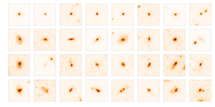
Figure 1: H band cutouts of visually classified galaxies as bulges (top row), disks (second row), irregular disks (third row) and mergers (bottom row). The stamp size is $4.5^{"}\times 4.5^{"}$.

2.2 Low-redshift comparison sample

One of the purposes of this study is to explore the structural evolution of galaxies across cosmic time. To study this evolution, we will compare the ERS population to a sample of $\sim 14000$ nearby ($z<0.1$) galaxies, drawn from the SDSS, which have been visually inspected by Nair & Abraham (2010, NA10 hereafter). To the NA10 sample, we add a subsample of visually classified mergers from the Galaxy Zoo project. To create a set of comparable images, we place the $g$-band images of the NA10 galaxies at high redshift (following the same redshift and magnitude distribution of the ERS sample in Windhorst et al., 2011) and convolve them with a gaussian to match the ERS FWHM before adding an average ERS background (see Huertas-Company et al. 2008, 2009 for more details). Morphological parameters are then estimated from these simulated images in an identical fashion to the real ERS galaxies (see section 2.1.3). The stamps from the NA10 sample used for this work are available at gepicom04.obspm.fr/. We refer readers to Pović et al. (2013) for a detailed description of how the stamps were created. We note that no physical evolution is included when redshifting these galaxies, but the observing conditions are preserved, making this sample well-suited to study the evolution of morphological parameters from $z\simeq 0$ to $z\simeq 3$.

3 Non-parametric morphologies of galaxies at $1<z<3$

3.1 Distribution of morphological classes in classical 2-D planes at $1<z<3$

We begin by exploring the general behaviour of the morphological parameters for different visually-identified morphological classes at $z>1$. Figures 2 and 3 present the distribution of visual morphological classes in the $(C-A)$, $(G-M_{20})$, $(C-S)$, $(C-e)$, $(n-e)$ and $(n-C)$ parameter planes in two redshift bins ($1<z<2$ and $2<z<3$) respectively.

As is the case at low redshift (e.g Huertas-Company et al. 2011), the $(C-A)$ plane indicates that spheroids are more concentrated than the other morphological classes , but with large scatter ($\tilde{C}_{bulge}\sim 2.7\pm 0.3$, $\tilde{C}_{disk}\sim 2.3\pm 0.3$). A simple selection based on concentration (i.e. $C>2.5$) for bulges will hence result in a poor classification since only $70\%$ of the bulges have concentration larger than 2.5 and almost $30\%$ fall also in this region. While the median asymmetry in the merger class (66% of mergers have $A>0.2$) is also higher than that in regular galaxies ($\tilde{A}_{disks+bulges}\sim 0.11\pm 0.05$), it is apparent that many ($>30\%$) late-type galaxies (especially irregular disks) also exhibit high asymmetry values (see $C-A$ plane). This makes extremely difficult to cleanly separate these morphological types using parameters alone (see section 4).

In the $G-M_{20}$ plane, spheroids are again reasonably well separated in $G$ ($\tilde{G}_{bulge}\sim 0.56\pm 0.05$ vs. $\tilde{G}_{disk}\sim 0.46\pm 0.05$). However, M₂₀ does not appear to provide an efficient route for identifying irregular/merger objects at $z>1$ at least when only the median values are considered ($\tilde{M}_{20-regular}\simeq\tilde{M}_{20-irregular}\sim-1.49$ ). A more detailed analysis is presented in section 4. The clumpiness parameter $S$ appears to be slightly more sensitive to irregularities in the galaxy structure as shown in the $C-S$ plane ($\tilde{S}_{regular}\sim 0.02\pm 0.02$ and $\tilde{S}_{regular}\sim 0.04\pm 0.02$) but not discriminant enough by itself. There are in fact a significant fraction of regular galaxies with relatively high clumpiness values and also an important number of galaxies for which the clumpiness is close to $0$ (fig. 2) of both morphological types. Recall that the clumpiness is close to $0$ when the galaxy has no high frequency structure which means that the light profile is smooth or unresolved.

The ellipticity parameter (see $C-e$ and $n-e$ planes) at $z>1$ behaves similarly to the situation at low redshift, with disk-dominated galaxies being more elongated than bulges ($\tilde{e}_{bulge}\sim 0.18$, $\tilde{e}_{disk}\sim 0.36$). Finally, the Sersic index correlates well with the concentration as expected and most disk galaxies show Sersic indices lower than 2.5 (similar to their counterparts in the local Universe). However, it is worth noting that $>30\%$ of spheroids also show such low Sersic values, implying that a morphological selection based exclusively on this parameter, will have significant contamination as extensively showed in previous works (e.g Mei et al., 2012).

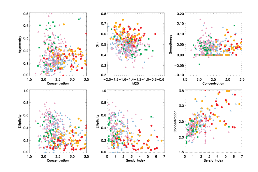
Figure 2: 2D morphological planes for visually classified galaxies with $1<z<2$. Red circles are bulges without disk, orange circles are bulge dominated galaxies with a faint disk, blue triangles are regular disks, magenta triangles indicate disturbed disks and green squares show mergers.

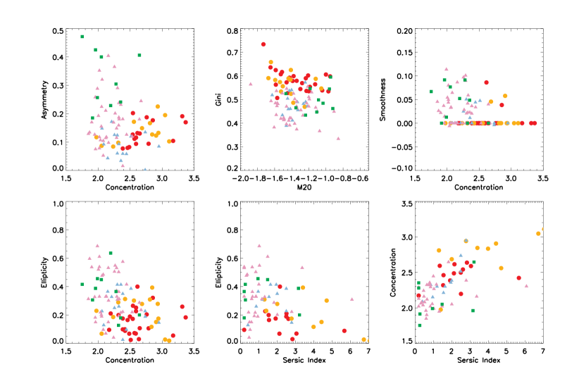
Figure 3: 2D morphological planes for visually classified galaxies with $2<z<3$. Red circles are bulges without disk, orange circles are bulge dominated galaxies with a faint disk, blue triangles are regular disks, magenta triangles indicate disturbed disks and green squares show mergers.

3.2 Dependence of morphological parameters on wavelength

The high-resolution HST images now available span both optical and near-infrared filter sets, which trace the rest-frame UV and optical at $z>1$ respectively at a very similar depth (Windhorst et al., 2011) It is desirable to quantify the statistical variation in the derived values of morphological parameters with wavelength. In Figure 4, we compare values of our morphological parameters for the same objects, measured in the $F775W$ (i band) filter (rest-frame UV at $z\simeq 2$) and the $F160W$ filter (rest-frame optical at $z\simeq 2$). Since both images do not have the same FWHM ($0.077^{"}$ vs. $0.150^{"}$), we first convolve the $F775W$ with a gaussian filter with a quadrature difference $FWHM\sim 0.125$ to match the resolution of the $F160W$ and get rid of any resolution effect on the derived parameters. We also used the segmentation maps obtained in the H band to compute the morphological parameters in the i band to make sure that we consider the same physical area in each galaxy. Recall that we only show the galaxies for which parameters were properly computed in both photometric bands so the number of objects in each panel might differ.

Overall, morphological parameters exhibit a correlation in the two filters. The parameters that measure concentration ($C$, $G$, $M_{20}$), exhibit a good correlation with small scatter in the two filters, with typical variations in the median values of less than $10\%$ and a Pearson correlation coefficient of $\rho\simeq 0.8$. We notice that Lee et al. (2013) reported a significant systematic offset in the Gini coefficient between rest-frame UV and optical which we do not find here. Parameters that are specially sensitive to the internal structure of the galaxy, such as asymmetry ($A$) and clumpiness ($S$), appear to be more wavelength dependent. Indeed, the correlation between these parameters measured in the rest-frame optical and UV appears very weak ($\rho\simeq 0.4$), as indicated in Figure 4.

In terms of our broad morphological classes (ETGs and LTGs), we find that later types are more affected by the morphological k-correction, with LTGs being $\sim 50\%$ more asymmetric and $\sim 40\%$ more clumpy in the rest-frame UV than in the rest-frame optical. We notice however that the median clumpiness also changes very significantly ($>100\%$) between the i and H band for ETGs. This is explained because the median value in te H band is almost $0$ for these objects while there are a few objects in the i band which present larger values which make the relative increase very large. Finally, we also find a trend for irregular and disk galaxies to have lower $M_{20}$ coefficients in the i band as reported by Lee et al. (2013), which is also a consequence of their more patchy morphology. These results confirm similar results already obtained in the local universe (e.g. Taylor-Mager et al., 2007; Windhorst et al., 2002) and also highlight the importance of recalibrating morphological proxies each time a different set of filters is used. Indeed, it is also worth considering whether a classification that combines the same parameters measured in different wavelength may yield a more robust automated classification. We explore this issue in Section 6.

It is important to notice an important caveat when interpreting the differences in the morphological parameters from one filter to the other in terms of physical differences, since the parameters are in fact very sensitive to the image quality (S/N, FWHM…, e.g. Brinchmann et al., 1998; Bershady, Jangren & Conselice, 2000; Lisker, 2008; Robaina et al., 2009; Kartaltepe et al., 2010). Even though we have tried to make a fair comparison by matching the resolutions, the pixel scales and by using images of similar depth, galaxies in the i band will appear systematically fainter given the shape of the SED ($i-H$ is always positive for our H band selection) and therefore are observed with a lower S/N.

$\begin{array}[]{c c}\includegraphics[width=173.44534pt]{i_vs_H_C.ps}&\includegraphics[width=173.44534pt]{i_vs_H_A.ps}\\ \includegraphics[width=173.44534pt]{i_vs_H_gini.ps}&\includegraphics[width=173.44534pt]{i_vs_H_M20.ps}\\ \includegraphics[width=173.44534pt]{i_vs_H_S.ps}&\includegraphics[width=173.44534pt]{i_vs_H_E.ps}\\ \end{array}$

Figure 4: Comparison of morphological parameters measured in the i band and in the H band for different visually identified classes. Red circles show early-type galaxies, blue triangles regular late-type galaxies, violet triangles are irregular disks and green squares indicate mergers. The dashed lines show the one-to-one relation. The values for the ellipticities are identical since we use the same SExtractor ellipse parameters (see text for details). A small offset has been added to the clumpiness (bottom left panel) measured in the i band when it was too close to zero for visibility reasons. We also indicate in each panel the relative difference in the median values between the two filters.

3.3 Structural evolution from $z\sim 0$ to $z\sim 3$

In this section, we explore how galaxies in different morphological classes evolve structurally with look-back time. In Figure 5, we present the same morphological planes that were explored for the high redshift sample in the previous section, but this time for the local sample redshifted to high redshift (as described in Section 2.2). In this figure, for the high redshift galaxies, early-types are defined as those classified as bulges or bulges + faint disks, late-types are all regular disks and the irregular class contains both irregular disks and mergers as defined in section 2.1.4. For the local sample, early-type and late-type galaxies are galaxies with $T_{type}<0$ and $T_{type}>0$ according to the Nair & Abraham (2010) catalog. The irregular class contains the Galaxy Zoo mergers.

We find that, at first level, the behaviour of the local redshifted sample is similar to their counterparts at high redshift. Early-types are typically more concentrated than disk-dominated galaxies and mergers exhibit higher asymmetry values as would be expected at any epoch. However, they do not span exactly the same ranges. Since the measurement of parameters in the local and high redshift samples are done under the same conditions (i.e. pixel size, noise, etc.) any differences in the parameter values are a reflection of the structural changes in galaxies over time.

We quantify this structural evolution in Figures 6 and 7. We present the distributions of values for our morphological parameters, for both the high-redshift ERS sample and the local redshifted sample split into early-types and late-types respectively. The relative differences on the median values are summarized in Table 1. Generally, early-type systems show more evolution in their morphological parameters than their late-type counterparts. However, parameters measuring the internal structure (A and S) show the largest evolution in the redshift range probed here ($0<z<3$) regardless of morphological type. Galaxies are significantly more asymmetric at $z>1$, the increase in asymmetry being 100% (a factor of 2) for some early-type systems and LTGs are also significantly more clumpy at $z>1$. The relative variation of the median values of the clumpiness for ETGs shows a puzzling trend at first order. ETGs at $z>1$ are in fact $\simeq 100\%$ less clumpy than their local counterparts. This is again explained because a significant fraction of ETGs in the ERS fields have clumpiness values close to 0 (see fig. 6), which indicate that they have no structures or that they are too compact to resolve them. The evolution is less pronounced in the remaining parameters, with variations of $\sim 10\%$ for ETGs, and even lower for LTGs. Early-type galaxies at high redshift appear more concentrated, have lower $M_{20}$ values and higher Gini coefficients than their local counterparts. This is simply a reflection of the fact that early-types are more compact at high redshift (e.g. Daddi et al., 2005, Trujillo et al. 2006, Buitrago et al. 2008, Huertas-Company et al. 2013). Since our morphological measurements on the high redshift galaxies are performed under the same conditions as the local redshifted sample, the evolution in these parameters is a consequence of real evolution in the early-type population over cosmic time.

An important implication of our analysis is that a local sample of galaxies, simply redshifted to $z>1$ might not be a good template for measuring the morphological properties of galaxies at these epochs. In Section 4 below, we explore this further, by studying the accuracy of the classifications when such a local redshifted sample is used to calibrate automated classifiers (compared to using a real galaxy sample at high redshift).

$\begin{array}[]{c }\includegraphics[width=390.25534pt]{plots_morphology_local_redshifted_highz_C_A.ps}\\ \includegraphics[width=390.25534pt]{plots_morphology_local_redshifted_highz_G_M20.ps}\\ \includegraphics[width=390.25534pt]{plots_morphology_local_redshifted_highz_C_S.ps}\\ \includegraphics[width=390.25534pt]{plots_morphology_local_redshifted_highz_C_E.ps}\\ \end{array}$

Figure 5: Comparison of the distribution in four morphological planes for galaxies at $1<z<3$ (big dots) and local galaxies artificially redshifted (small dots) for three morphological classes as labelled.

Param	ETGs	LTGs
$\Delta C$	$0.15\pm 0.04$	$-0.04\pm 0.02$
$\Delta A$	$0.95\pm 0.14$	$0.69\pm 0.08$
$\Delta G$	$0.16\pm 0.02$	$0.04\pm 0.01$
$\Delta M_{20}$	$-0.12\pm 0.02$	$-0.08\pm 0.01$
$\Delta S$	$-1.00\pm 0.13$	$1.01\pm 0.18$
$\Delta e$	$-0.10\pm 0.07$	$0.01\pm 0.06$

Table 1: Relative variation of different morphological parameters between $z\sim 0$ and $z\sim 3$ early-type (left column) and late-type (right column) galaxies. $(\Delta X=(\tilde{X_{z>1}}-\tilde{X_{z=0}})/\tilde{X_{z=0}})$.

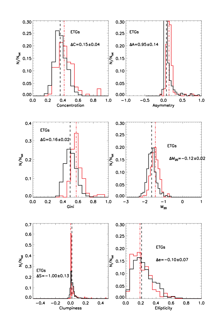
Figure 6: Distribution of morphological parameters for high redshift ETGs (red line) and local galaxies (black line) redshifted at the same redshift as explained in the text. For each parameter we provide the relative variation of the median value between $z\sim 3$ and $z\sim 0$, i.e. $\Delta=\frac{median_{z>1}-median_{z=0}}{median_{z=0}}$

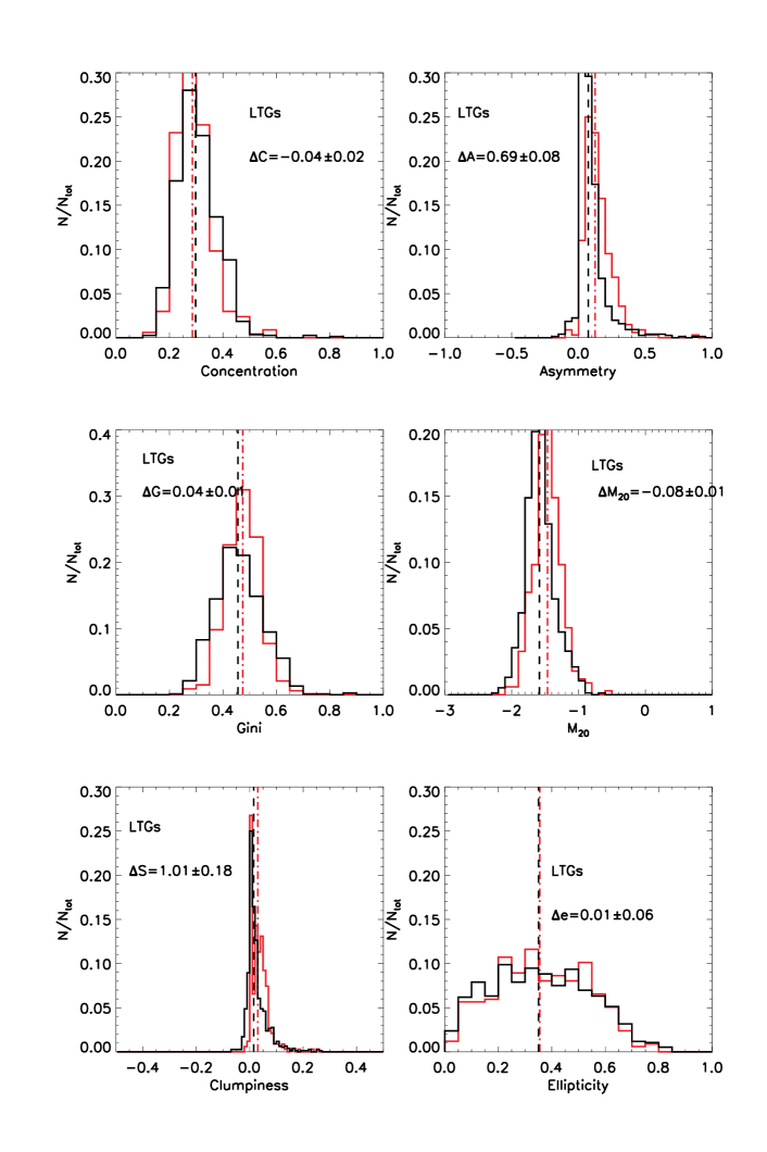
Figure 7: Distribution of morphological parameters for high redshift LTGs (red line) and local galaxies (black line) redshifted at the same redshift as explained in the text. For each parameter we provide the relative variation of the median value between $z\sim 3$ and $z\sim 0$, i.e. $\Delta=\frac{median_{z>1}-median_{z=0}}{median_{z=0}}$

4 Automated bayesian morphology at $z>1$ with galSVM

In this section we quantify the reliability of automated morphological classifications at $z>1$. Traditionally, combinations of morphological parameters have been shown to be sensitive to different morphological classes. For example, the $G$-M₂₀ plane has been used to identify merger candidates at low and intermediate redshift (see e.g. Lotz, Primack & Madau, 2004), while the $C$-$A$ plane has been used to discriminate between early-type and late-type galaxies (e.g. Conselice et al., 2003; Huertas-Company et al., 2008). Since the reliability of individual parameters can depend somewhat on factors such as signal-to-noise ratio, brightness and galaxy size (e.g. Brinchmann et al., 1998; Bershady, Jangren & Conselice, 2000; Lisker, 2008; Robaina et al., 2009; Kartaltepe et al., 2010), a multi-dimensional analysis that combines several parameters maximizes the accuracy of the parameter-based classification (Huertas-Company et al., 2008, 2011).

The galSVM code uses the information contained in several morphological parameters simultaneously, to associate a morphological class to an individual galaxy, by means of a Support Vector Machine (SVM). For this particular work, the galSVM classification simultaneously uses 7 parameters ($C$, $G$, $M_{20}$, $A$, $S$, $n$ and $e$). All parameters are measured in the $F160W$ filter (but in section 6 we explore the effects of adding parameters measured in shorter-wavelength bands).

Since the technique is optimized to classify only 2 morphological classes at a time, we perform two separate classifications. The first is aimed at distinguishing between broad morphological classes (LTG vs. ETG). The second attempts to differentiate irregular and merging galaxies from the regular classes. In essence, each galaxy in the sample is allocated two probabilities: $P_{ETG}$ (probability of being an early-type galaxy) and $P_{irr}$ (probability of being an irregular disk). galSVM is calibrated using a training sample of visually-classified morphologies, with the assumption that the morphologies in the training set are robust. For an individual galaxy, the code then measures an a posteriori probability for that object to belong to a given morphological class.

We note that a key requirement for accurate classification is that the training sample should be as close as possible to the real sample one wishes to classify. An approach used in previous works (e.g Huertas-Company et al. 2008, 2009) has been to use a local sample with high quality morphologies which are redshifted to the epoch of interest. However, our results in Section 5.2 indicate that, due to the evolution of morphological parameters between $z>1$ and the local Universe, redshifted local samples do not provide a good training set for studying galaxy morphologies in the early Universe.

For that reason, in this work we use 2 different training sets to train galSVM in order to calibrate the effects of the training on the final classification at $z>1$:

SDSS sample: Our first training set is the local SDSS comparison sample described in Section 2.2. Recall that, to create this comparison sample, SDSS galaxies from NA10 are redshifted, scaled in luminosity to account for cosmological dimming and placed in a real ERS background with the proper pixel scale. As noted before, the drawback of using this training set is that no morphological evolution is assumed i.e. the morphological structure of the redshifted dataset are identical to the local galaxy population. This approach has been used at $z<1$ without significant biases (e.g. Pović et al., 2013; Huertas-Company et al., 2013). However, as shown in section 3.3, there is significant evolution of the morphological parameters between $z\sim 0$ and $z\sim 3$, which might induce important effects in the final classification at $z>1$. By employing this training set, we wish to explicitly calibrate the effects of using redshifted local samples as training sets for morphological work in the early Universe.

High redshift sample: As described in section 2.1.4, the main sample used for this work has been visually classified directly on the H-band ERS images. This training set should be considered the best case, since we are using data at the same epoch for both the training and classification. Note, however that there is a certain amount of redundancy in this exercise, since there is a significant overlap between the datasets used for both the training and the automated classification. To explore the impact of this redundancy, we check our classification results against the visual classification recently performed by the CANDELS team (Kartaltepe et al., 2014 - see section 5).

4.1 Classification of broad morphological types

We begin by investigating how broad morphological classes, i.e. bulge-dominated and disk-dominated galaxies, are recovered using galSVM. For galaxies visually classified as LTGs and ETGs, Figure 8 shows the probability of these galaxies to be classified as early-type by galSVM. The left-hand panel shows results obtained using a high-redshift galaxy sample as the training set, while the right-hand panel shows the corresponding distributions with the local redshifted sample used as a training set.

For the results obtained using the high-redshift training set, we find good agreement between visual and automated classifications at $z>1$. The probability distribution for visually-classified ETGs clearly peaks at high values of p_ETG from galSVM, while visually-classified LTGs show a peak at low values of p_ETG. When the SDSS sample is used for training (right panel), we still see the two peaks but the distributions exhibit more extended wings. This is especially true for the early-type population, which contains a considerable fraction of galaxies with low p_ETG probabilities.

As noted before, the advantage of an SVM-based classification is that it provides a probability rather than a binary classification. It is therefore possible to tune the selection of a particular morphological class using different probability thresholds, depending on the actual science goals. The most natural selection would be to include in a given class, all objects that have a probability greater than 0.5, but it is possible to change the threshold depending on the properties (e.g. purity/completeness) required of the sample.

We proceed by quantifying the ‘purity’ and ‘completeness’ of the galSVM classifications,taking the visual classifications as reference. For a given probability threshold ($p_{th}$), we define the following quantities:

• True positives (tp): # galaxies with $p_{ETG}>p_{th}$ ($p_{LTG}>p_{th}$) which are visually classified as early-type (late-type).

• True negatives (tn): # galaxies with $p_{ETG}<p_{th}$ ($p_{LTG}<p_{th}$) which are visually classified as late-type (early-type).

• False positives (fp): # galaxies with $p_{ETG}>p_{th}$ ($p_{LTG}>p_{th}$) which are visually classified as late-type (early-type).

• False negatives (fn): # galaxies with $p_{ETG}<p_{th}$ ($p_{LTG}<p_{th}$) which are visually classified early-type (late-type).

The purity P, also known as reliability (the fraction of well-classified objects among all objects classified in a given class) and the completeness C (the fraction of well-classified objects among all objects really belonging to a given class) are then defined as follows:

$$P=1-\frac{fp}{fp+tp}$$ (3)

$$C=\frac{tp}{fn+tp}$$ (4)

P (Purity) effectively measures the level of contamination in the automated classification. For example, if $30\%$ of the galaxies classified by galSVM as ETGs are, in fact, classified as LTG via visual inspection, then the purity of the galSVM-classified sample will be $70\%$. C (Completeness), on the other hand, measures how well galSVM recovers objects in a visually-classified class. For example, if $C=100\%$ for a sample of galaxies classified as ETGs by galSVM, then this indicates that all galaxies visually classified as ETGs are recovered as such by the automatic classification. A perfect classification is, therefore, $100\%$ pure and $100\%$ complete. In practice, there is a tradeoff between the two quantities, since requiring better completeness typically involves increasing the level of contamination in the automated results.

In Table 2 we present the completeness and purity of samples selected with different probability thresholds, using the local and the high-redshift training sets. Not unexpectedly, an increase in the probability threshold results in a purer sample while the completeness decreases. This is particularly true for the ETG population. To achieve a purity greater than $80\%$, we need to select galaxies with $p_{ETG}>0.7$, for which the completeness then drops to $\sim 60\%$. Generally speaking, late-type galaxies are more easily recovered with automated proxies. For example, selecting galaxies with $p_{LTG}>0.4$ leads to a sample that is 90% complete and $90\%$ pure. This is largely a consequence of spatial resolution. Galaxies that are clearly extended are easily identified as disk dominated galaxies. However, the most compact disk galaxies tend to contaminate the early-type population. This effect might be reduced if higher resolution images are used. The ERS images have been resampled to a pixel size of $0.09^{"}$ but images resampled at a resolution of $0.06^{"}$ are now available which might help in resolving compact LTGs. This will be explored in a future work. It is worth noting though that, given that the number of late-type systems at $z>1$ is significantly higher than the number of early-type galaxies, the misclassification of a small proportion of LTGs has a relatively insignificant impact on the recovery of the general population of LTGs. Some examples of the galaxies classified automatically are shown in figure 9.

In Table 2, we quantify the effect of the training set used for the galSVM classifications. The accuracy of the automated classification decreases when a redshifted sample from the SDSS is used for training, as opposed to a sample of real high-redshift galaxies. This is expected since, as described in Section 3.3, the morphological parameters used for the classification show some evolution from low to high redshift. Thus, local galaxies are not the optimal template for classifying a high-redshift ($z>1$) sample. This discrepancy between a local and (real) high-redshift sample is particularly critical for the SVM, which is a machine learning technique that is particularly sensitive to the training set. Interestingly, the effect of the training set is reflected more in the completeness - for example, a threshold value of $p>0.6$ in the ETG probability yields a completeness of $57\%$ when measured using a low-redshift SDSS training set, while $\sim 70-80\%$ is achieved using a training set of actual high-redshift galaxies.

Recall that an increase in the probability threshold results in a purer sample which is typically less complete. A low completeness might have critical consequences for the scientific conclusions derived, if the selected sample is biased towards a specific population. For instance, one might wonder if galaxies with higher probability values are the brightest and/or the largest and/or the ones with higher surface brightnesses, as a result skewing the science results. In Figure 10 we address this issue by plotting the size (from galfit), magnitude and surface-brightness distributions of early and late-type samples selected with increasing probability thresholds (0.3, 0.5 and 0.7). The main conclusion is that there is no apparent bias in the main properties of the selected samples i.e the distributions are similar ($P_{K-S}>0.8$ - see fig. 10), independent of the probability threshold applied. This result reflects the fact that the morphological parameters used for the automated classification are reliable enough in the ranges of magnitudes, surface brightnesses and sizes explored in this study (note that we are limited to $H<24$, where visual classifications are reliable), that the probability is not correlated with any of this physical parameters.

$\begin{array}[]{c c}\includegraphics[width=216.81pt]{histograms_visual_broad_petg.ps}&\includegraphics[width=216.81pt]{histograms_visual_broad_petg_SDSS.ps}\\ \end{array}$

Figure 8: ETG Probability distribution for visually classified early-type (red) and late-type (blue) galaxies. The left panel shows the distributions obtained with a high-z training set and the left panel those obtained with a local sample (see text for details).

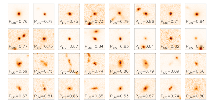
Figure 9: H band cutouts of automatically classified early-type galaxies (2 top rows) and late-type (2 bottom rows). ETGs (LTGs) are selected with a probability threshold of $p>0.7$ ($p>0.5$) which results in a contamination of $\sim 15\%$ ($<10\%$). See text for details. The associated probability is indicated in each individual stamp.

$P_{thresh}$	$P^{ERS}(ERS)$	$C^{ERS}(ERS)$	$P^{SDSS}(ERS)$	$C^{SDSS}(ERS)$
ETGs
0.3	53.68	99.03	48.80	89.71
0.4	62.50	92.23	56.61	78.68
0.5	70.45	90.29	66.42	66.91
0.6	78.70	82.52	71.56	57.35
0.7	80.00	66.02	77.11	47.06
0.8	83.02	42.72	85.96	36.03
LTGs
0.3	88.41	94.01	83.18	95.77
0.4	93.55	91.90	85.67	92.61
0.5	96.08	86.27	88.07	88.38
0.6	96.60	79.93	91.46	79.23
0.7	99.49	69.01	95.52	67.61
0.8	100.00	45.77	97.58	42.61
Irr/mergers
0.3	67.89	97.66	54.37	87.67
0.4	73.06	93.57	63.60	73.13
0.5	76.92	87.72	75.69	60.35
0.6	81.18	80.70	79.85	47.14
0.7	85.11	70.18	85.06	32.60
0.8	87.25	52.05	85.42	18.06

Table 2: Completeness (C) and purity (P) for ETGs, LTGs and irregulars at $1<z<3$ in the ERS obtained with a high redshift (ERS, first 2 columns) and low redshift (SDSS, last 2 columns) training sets (see text for details).

$\begin{array}[]{c c}\includegraphics[width=202.35622pt]{histograms_pthresh_sb_ETGs.ps}&\includegraphics[width=202.35622pt]{histograms_pthresh_sb_LTGs.ps}\\ \includegraphics[width=202.35622pt]{histograms_pthresh_mag_ETGs.ps}&\includegraphics[width=202.35622pt]{histograms_pthresh_mag_LTGs.ps}\\ \includegraphics[width=202.35622pt]{histograms_pthresh_re_ETGs.ps}&\includegraphics[width=202.35622pt]{histograms_pthresh_re_LTGs.ps}\\ \end{array}$

Figure 10: Surface brightness (top row), magnitude (middle row) and size (bottom row) distributions for early-type (left column) and late-type galaxies, selected with different probability thresholds. An increase in the probability threshold does not introduce significant biases in the selected galaxy population. The probability of the K-S test between the $p_{th}>0.3$ and $p_{th}>0.7$ sample is indicated in each panel.

4.2 Recovering finer morphological types: irregular disks/mergers

We proceed by investigating how the automated classifications perform in recovering finer morphological classes, in particular mergers and irregular disks. Figure 11 shows the galSVM-derived probability for galaxies to be irregular or merger using both the local and high redshift training sets. For this exercise, the local training set consists of visually-identified mergers from Galaxy Zoo, while the high-redshift training set was constructed by combining the irregular disks and merger classes, both due to a lack of statistics and also because, as shown in Section 2.1.4, the distinction between these two classes is challenging to produce even visually.

The left-hand panel of Figure 11 shows that ETGs have very low galSVM probabilities of being irregular, while visually-classified mergers and irregular disks have larger probabilities. galSVM is, therefore, able to distinguish irregular objects from ETGs with good accuracy. The regular LTG population, however, does have a broader probability distribution, which is a reflection of the fact that the general population of late-type galaxies at $z>1$ tends to be more asymmetric than in the local Universe, as shown in section 3.3. The accuracy of the classification for different probability thresholds is quantified in Table 2, which shows that irregular objects can be recovered by galSVM with a (low) contamination of $\sim 20\%$ and a (fairly high) completeness of $\sim 80\%$. Some example images of galaxies automatically classified as irregular are shown in figure 12

We also explore the effect of the training set used on the recovery of mergers and irregular disks at $z>1$. The right-hand panel of Figure 11 shows the galSVM-derived probability for a galaxy to be irregular, obtained using the low-redshift (SDSS) training set. While the general trends are preserved, the probability distribution for the merger class is broader than the one obtained with the high redshift training set. This is driven by the fact that the population of mergers and irregular disks observed at high redshift do not have direct analogues in the local Universe. Hence, the training set lack good ‘templates’ for these objects which are required to train the SVM accurately. This has an obvious impact on the final classification, especially in terms of the completeness, as can be seen in Table 2. In other words, for the same probability threshold, the completeness is $\sim 20\%$ less with a local training sample than with the high redshift training set.

$\begin{array}[]{c c}\includegraphics[width=216.81pt]{histograms_visual_irr.ps}&\includegraphics[width=216.81pt]{histograms_visual_irr_SDSS.ps}\\ \end{array}$

Figure 11: Irregular/merger probability distribution for visually identified morphological types as labelled. The left panel shows the result when a high z training sample is used and the right panel the result with the SDSS dataset.

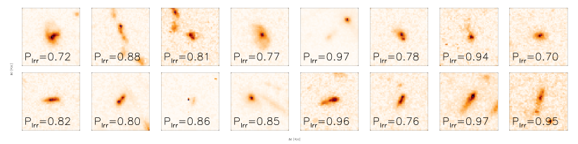
Figure 12: H band cutouts of automatically classified irregular/merger galaxies selected with a probability threshold $p>0.7$ (i.e. $\sim 15\%$ contaminations). The associated probability is indicated in each individual stamp.

5 Comparison with CANDELS visual classifications

Recently, the CANDELS team (PIs Faber & Ferguson; see Grogin et al. 2011, Koekemoer et al. 2011) has performed a detailed visual classification of galaxies in the GOODS-S field (Kartaltepe et al., 2014) using the H-band WFC3 observations down to $H<24.5$. In this significant effort, 65 individual classifiers contributed to the morphological classification (being 3-5 the average number of classifiers per galaxy) who are asked to provide a number of flags related to the galaxy’s structure, morphological k-correction, interaction status and clumpiness. As a result, each galaxy in the catalog has an associated fraction of classifiers who have selected a given flag which can be used to define morphological classes. This dataset is therefore an excellent independent test to assess the accuracy of the automated classification scheme presented in this work.

Following Kartaltepe et al. (2014), we first define 4 morphological classes - mostly disks, mostly spheroids, disk + spheroid and irregulars - based on the fractions:

• Mostly disks are those galaxies for which less than 2/3 of the classifiers selected them as spheroids and more than 2/3 selected them as disks.

• Mostly spheroids are those for which more than 2/3 voted for a spheroid and less than 2/3 for a disk.

• The disk + spheroid class contains galaxies that were labelled as spheroids and disk by more than 2/3 of the classifiers.

• Finally, the irregular class is made of galaxies identified as irregular by more than 2/3 of the classifiers and for which less than 2/3 selected them as disks or spheroids.

These classes should roughly correspond with the visual classes selected in this work (see section 2.1.4). Recall, however, that our visual classification above defined an ‘irregular disk’ class which might not be in these 4 CANDELS classes just described. In order to cope with this, we split the mostly disks class into asymmetric and regular objects using the $f_{asym}$ fraction (lower and larger than $2/3$) which provides the fraction of classifiers that label the galaxy as irregular.

We then perform 2 different tests. First, we simply calibrate the effect of using different visual classifications to estimate the accuracy of the classifier, by plotting the distribution of the probabilities (‘trained’ on the ERS bases classes described in section 2.1.4) of being labelled as ETG (left panel) and irregular (right panel) for the ERS galaxies but for the 5 visually defined classes in CANDELS as explained above (Figure 13). The purpose of this test is to estimate the robustness of the automated and visual classifications but we still keep a redundancy in the training and testing sets. We recover the expected trends confirming the results of previous sections. All disk dominated galaxies (disks, irregulars and disk irregulars) present low probabilities to be ETG while the spheroid class has high values. Broad morphological types are therefore well recovered at $z>1$. Interestingly, the bulge+disk class from CANDELS has large probabilities to be ETG according to galSVM, which means that the bulge component is dominating the computation of the morphological parameters. Concerning the irregular galaxies, the right panel of figure 13 confirms the trends observed in the previous sections. Galaxies visually classified as irregular by the CANDELS team exhibit a peak at large galSVM probabilities to be irregular. However, early-type galaxies peak at low probabilities, which confirms the fact that irregulars can indeed be easily separated from ETGs. As was the case for the our visual classifications based on the ERS, the regular disk class presents a flat distribution and will therefore pollute the automatically selected class of irregulars. These trends are quantified in the first 2 columns of table 3 in terms of purity and completeness, as in previous sections. We note that the values for the three morphological classes are comparable to the values reported using our ERS visual classification above. The main conclusion of this test is that visual classifications are robust enough so that the accuracy of the automated classification is not significantly affected.

$\begin{array}[]{c c}\includegraphics[width=216.81pt]{histograms_candels_PETG.ps}&\includegraphics[width=216.81pt]{histograms_candels_PIRR.ps}\\ \end{array}$

Figure 13: Comparison of the automated classification on the ERS sample with the CANDELS visual classification. Left panel: probability distribution to be ETG for different visually identified morphological types in CANDELS as labelled (see text for details). Galaxies visually classified as spheroids have large probabilities to be ETG. The Spheroid+Bulge class tends to have also high probabilities. Right panel: probability distribution to be irregular for different visually identified morphological types in CANDELS as labelled (see text for details). Galaxies visually classified as irregulars have large probabilities to be irregular according to the automated scheme presented in this work. The contamination comes mostly form the disk class (blue dashed line).

The CANDELS sample allows however a more crucial test regarding the independence of the training set. So far, we have used overlapping samples for training and classifying as explained in section 4, which necessarily leads to a best case solution. The main purpose of automated classification schemes however is to be used massively in a large dataset for which visual classification are available only for a small fraction of the sample. We now split the full CANDELS morphological catalog in two independent subsets and use one for training and the other for testing (with the CANDELS visual classes as training labels). We select galaxies with $H<24$ and $1<z<3$ in the GOODS-S area with visual morphologies from the catalogs of Kartaltepe et al. (2014) (i.e. 1717 objects). The photometric redshifts for this sample are taken from the 3D-HST public release v4.1(Skelton et al., 2014; Brammer et al., 2012) This test should therefore calibrate the effect of the redundancy on the training set. Results are shown in figure 14 and quantified in table 3. We again recover very similar trends, (especially for the early-type class) to the ones already discussed, which proves that the classification is robust even when independent datasests are used for training and testing. Interestingly, the behavior of the irregular class slightly changes and the peak at large probabilities becomes less pronounced resulting in a smaller completeness (see table 3). This certainly needs to be investigated more carefully in future work but it might be a reflection of the fact that the irregular class is less well definded than other classes (in visual classifications) and hence the learning machine tends to be very training set dependent. It could also be an effect of S/N since the CANDELS are shallower on average than the ERS.

$\begin{array}[]{c c}\includegraphics[width=216.81pt]{histograms_candels_PETG_ALL_CTRAIN.ps}&\includegraphics[width=216.81pt]{histograms_candels_PIRR_ALL_CTRAIN.ps}\\ \end{array}$

Figure 14: Comparison of CANDELS automated classification trained on the CANDELS visual classification using an independent subsample. Left panel: probability distribution to be ETG for different visually identified morphological types in CANDELS as labelled (see text for details). Galaxies visually classified as spheroids have large probabilities to be ETG. The Spheroid+Bulge class tends to have also high probabilities. Right panel: probability distribution to be irregular for different visually identified morphological types in CANDELS as labelled (see text for details). Galaxies visually classified as irregulars have large probabilities to be irregular according to the automated scheme presented in this work. The contamination comes mostly form the disk class (blue dashed line).

$P_{thresh}$	$P^{ERS}(CANDELS)$	$C^{ERS}(CANDELS)$	$P^{CANDELS}(CANDELS)$	$C^{CANDELS}(CANDELS)$
ETGs
0.3	50.93	92.44	58.45	92.83
0.4	57.61	89.08	64.54	89.14
0.5	66.67	85.71	69.41	84.63
0.6	73.64	79.83	73.50	80.12
0.7	78.43	67.23	79.55	72.54
0.8	91.53	45.38	86.39	59.84
LTGs
0.3	88.39	93.10	86.75	90.60
0.4	92.23	89.34	89.50	85.43
0.5	94.04	84.01	91.29	81.20
0.6	94.88	75.55	93.22	75.31
0.7	95.95	66.77	94.86	66.74
0.8	96.89	48.90	95.88	55.27
Irr/mergers
0.3	55.63	90.80	47.05	94.21
0.4	58.57	84.48	52.97	85.30
0.5	62.96	78.16	60.73	73.72
0.6	67.21	70.69	67.25	59.47
0.7	72.00	62.07	77.47	43.65
0.8	73.15	45.40	83.85	24.28

Table 3: Purity (P) and Completeness (C) for ETGs, LTGs and irregulars computed with the CANDELS visual classifications (Kaltartepe et al. 2014) with an ERS training set (first 2 columns) and a CANDELS independent dataset (last 2 columns) (see text for details). The superscript indicates the training set used and the name in the brackets the classified sample

6 Multi-wavelength classification

In this section we explore how the performance of the automated classifications changes when we use information in different wavelengths.

6.1 UV vs. optical

At $z>1$, the NIR filters on the HST trace the rest-frame optical wavelengths, while the optical filters probe the rest-frame UV. In Section 3.2 we showed that there are moderate variations in the values of our morphological parameters depending on the wavelength being employed to measure their values. We now quantify how the galSVM classifications respond to a change in wavelength. Figure 15 presents the galSVM-derived probabilities of galaxies to be classified as ETG and irregular, obtained for the same objects with parameters measured in the $H$ and $i$ bands (which traces the rest-frame optical and UV respectively). The training set is the same for both classifications, i.e. visual classifications performed in the $H$ band using the ERS.

We find a good correlation between the galSVM-derived probabilities based on different wavelengths. Galaxies with high probabilities to be ETG in the $H$ band generally have high probabilities to be ETG in the $i$ band. In fact, the best fit line between the two probabilities gives almost a one to one relation, i.e. $p_{ETG}^{i}=(1.1\pm 0.04)\times p_{ETG}^{H}-(0.05\pm 0.01)$ and the scatter of $\sim 0.2$. A similar behaviour is observed for irregular galaxies but the best fine line has a slope $<1$, i.e. $p_{irr}^{i}=(0.73\pm 0.02)\times p_{irr}^{H}+0.13\pm 0.01)$. There are however a few ($<2\%$) outliers which present high (low) probabilities to be ETG in the $H$ band and high (low) in the $i$ band. The differences in the classifications appear not to be a consequence of the difference in the shape of the two filters. As a matter of fact, the values of the morphological parameters used for the classification are very similar in both filters most of the times. The discrepancy in the final classification would be better explained by a failure in the algorithm, i.e outliers, that will be carefully explored in future work.

6.2 H+i classification

We now explore the effect of simultaneously using morphological parameters measured in the $H$ and $i$ bands on the galSVM classifications. Table 4 summarizes the purity and completeness of early and late-type galaxy samples obtained. Interestingly, we do not detect a significant change in the accuracy of the final classification when these additional parameters are included. Since, as shown in Section 3.2, there is a strong correlation between parameters measured in the two filters, using parameters measured in both bands does not add enough information to increase the quality of the classification. We obtain similar results when more than two filters are used. This, however, indicates the robustness of SVM to a redundancy in the data since, despite the inclusion of highly redundant parameters, the accuracy of the classification remains unaltered.

6.3 Adding additional no-morphological information: stellar mass

We conclude this section by exploring if the accuracy of the final classification can be improved by adding additional information derived from the spectral energy distribution of the galaxies, in this case the stellar mass. We re-classify the full sample using the main morphological parameters measured in the $H$ band adding stellar mass as an extra parameter keeping the same training set based exclusively on the visual aspect of the galaxy. In other words, the information brought by the stellar mass is used a posteriori, to check if better accuracy can be reached. The results in terms of purity and completeness are summarized in Table 5, for early and late-type galaxies. The inclusion of the stellar mass in the classification process tends to increase the completeness of the final classification, especially for the early-type population. For an equivalent probability threshold, e.g. P$\sim$0.6, a classification which uses the stellar mass is $\sim$10% more complete.

$\begin{array}[]{c c}\includegraphics[width=216.81pt]{pietg_pHetg.ps}&\includegraphics[width=216.81pt]{pietg_pHirr.ps}\\ \end{array}$

Figure 15: Probability to be ETG derived in the H band vs. the same probability derived in the i band (left panel). The right panel shows the probabilities to be irregular derived in the H and i band. The red dashed-dotted line shows the best fit line.

$P_{thresh}$	P	C
ETGs
0.3	49.07	96.34
0.4	57.14	92.68
0.5	63.79	90.24
0.6	70.71	85.37
0.7	78.48	75.61
0.8	80.30	64.63
LTGs
0.3	92.00	93.12
0.4	94.78	88.26
0.5	96.24	83.00
0.6	96.94	76.92
0.7	98.21	66.80
0.8	99.25	53.85

Table 4: Purity (P) and Completeness (C) for ETGs classified using parameters measured in the H and i band simultaneously (see text for details)

$P_{thresh}$	P	C
ETGs
0.3	70.69	98.80
0.4	76.70	95.18
0.5	81.25	93.98
0.6	84.88	87.95
0.7	86.25	83.13
0.8	86.49	77.11
LTGs
0.3	91.62	93.29
0.4	93.79	92.07
0.5	96.69	89.02
0.6	97.22	85.37
0.7	99.24	79.27

Table 5: Completeness and purity for ETGs classified using parameters measured in the H and the stellar mass simultaneously (see text for details)

7 Summary

We have studied the morphologies of 628 bright ($H<24$ mag) galaxies in the redshift range ($1<z<3$), using both visual inspection of images and commonly-used morphological parameters - Concentration ($C$), Asymmetry ($A$), the Gini coefficient ($G$) and $M_{2}0$.

The overall aim of this paper has been to quantify how different morphological classes evolve structurally over 90% of cosmic time and how well morphological parameters recover these classes at $z>1$, compared to visual inspection.

1. In the first part of this paper, we have studied the general behaviour of usual morphological proxies (i.e. C, A, S, G, $M_{20}$) at $z>1$, as well as their wavelength dependence and redshift evolution:

   • Generally speaking, the behaviour of morphological parameters at $z>1$ is similar to that at low redshift, in the sense that bulge-dominated galaxies are more concentrated and less asymmetric than disk dominated galaxies, with mergers and irregular disks being highly asymmetric.

   • By artificially redshifting local galaxies, we have measured the evolution of the morphological parameters with redshift. All parameters except asymmetry show moderate redshift evolution. At $z>1$, galaxies are $>50\%$ more asymmetric, have $\sim 10\%$ larger Gini coefficients and 10% lower M20 values than at $z=0$. The evolution is more pronounced for the early-type population.

   • There is a good correlation between parameters measured in the rest-frame optical and UV wavelengths, especially for ETGs. Late-type galaxies tend to be more asymmetric and more clumpy when observed in the UV rest-frame by $40-50\%$.

2. In the second part of this paper, we have explored the ability of automated parameters to recover morphological classes. We have applied the support vector machine based code galSVM to the full sample, using all the morphological parameters simultaneously and two different training sets (one local and one at high redshift) and have derived probabilities of being ETG, LTG and Irregular/merger for individual galaxies.

   • Early-type galaxies can be recovered automatically with a contamination of $<20\%$ and a completeness of $\sim 80\%$. For LTGs, less than $5\%$ contamination is measured with a completeness of $90\%$ depending on the probability threshold applied.

   • Irregular classes and mergers can be recovered with a purity of $\sim 70\%$. The contamination mainly derives from disk galaxies which are typically more irregular at $z>1$ than in the local Universe.

   • The accuracy of the classification decreases when a local training set based on the SDSS is used. This is a consequence of the evolution of the morphological parameters. This is especially critical for the irregular classes.

   • The automatic classification presented in this work correlates well with the CANDELS visual classificiation. Similar values of completeness and purity as the ones shown above are obtained when the classification is either compared to the CANDELS morphologies keeping the same training set or when the classifier is trained using the CANDELS classifications.

   • There is a good correlation between the automated classification performed in the rest-frame optical and UV wavelengths with less than 2% galaxies presenting very different probabilities in the two filters.

   • Adding the stellar mass derived from the SED to the classifier such as the stellar mass and/or morphological parameters measured in different filters, tends to increase the slightly increase the completeness of the classification. A more detailed analysis will be performed in future work.

   Given the prodigious amount of data expected from future surveys such as EUCLID and LSST, a unified approach that combines both visual inspection and morphological parameters is desirable. Accurate visual inspections are necessary to properly train the algorithms and maximize the efficiency of the automatic procedures. However, we have shown that automated techniques, based on machine learning do a reasonable job in recovering morphological classes at $z>1$, including fine morphological classes (e.g. irregular/mergers). In forthcoming papers, we will provide a classification of all CANDELS fields with the procedure presented here. We will also explore new methodologies based on novel machine learning algorithms.

References

- Abraham et al. (1996) Abraham R. G., Tanvir N. R., Santiago B. X., Ellis R. S., Glazebrook K., van den Bergh S., 1996, MNRAS, 279, L47
- Abraham, van den Bergh & Nair (2003) Abraham R. G., van den Bergh S., Nair P., 2003, ApJ, 588, 218
- Ball et al. (2004) Ball N. M., Loveday J., Fukugita M., Nakamura O., Okamura S., Brinkmann J., Brunner R. J., 2004, MNRAS, 348, 1038
- Bell et al. (2004) Bell E. F., Wolf C., Meisenheimer K., et al., 2004, ApJ, 608, 752
- Bernardi et al. (2003) Bernardi M., Sheth R. K., Annis J., et al., 2003, AJ, 125, 1882
- Bershady, Jangren & Conselice (2000) Bershady M. A., Jangren A., Conselice C. J., 2000, AJ, 119, 2645
- Brammer, van Dokkum & Coppi (2008) Brammer G. B., van Dokkum P. G., Coppi P., 2008, ApJ, 686, 1503
- Brammer et al. (2012) Brammer G. B. et al., 2012, ApJS, 200, 13
- Brinchmann et al. (1998) Brinchmann J. et al., 1998, ApJ, 499, 112
- Bundy, Ellis & Conselice (2005) Bundy K., Ellis R. S., Conselice C. J., 2005, ApJ, 625, 621
- Cole et al. (2000) Cole S., Lacey C. G., Baugh C. M., Frenk C. S., 2000, MNRAS, 319, 168
- Conselice et al. (2003) Conselice C. J., Bershady M. A., Dickinson M., Papovich C., 2003, AJ, 126, 1183
- Conselice, Bershady & Jangren (2000) Conselice C. J., Bershady M. A., Jangren A., 2000, ApJ, 529, 886
- Conselice et al. (2011) Conselice C. J. et al., 2011, MNRAS, 413, 80
- Daddi et al. (2005) Daddi E. et al., 2005, ApJ, 626, 680
- Dekel et al. (2009) Dekel A. et al., 2009, Nature, 457, 451
- Dekel, Sari & Ceverino (2009) Dekel A., Sari R., Ceverino D., 2009, ApJ, 703, 785
- Ellis et al. (1997) Ellis R. S., Smail I., Dressler A., Couche W. J., Oemler A. J., Butcher H., Sharples R. M., 1997, ApJ, 483, 582
- Faber et al. (2007) Faber S. M., Willmer C. N. A., Wolf C., et al., 2007, ApJ, 665, 265
- Ferreras et al. (2009) Ferreras I. et al., 2009, ApJ, 706, 158
- Fukugita et al. (2007) Fukugita M. et al., 2007, AJ, 134, 579
- Giavalisco, & et al. (2004) Giavalisco M., , et al., 2004, ApJ, 600, L93
- Grogin et al. (2011) Grogin N. A. et al., 2011, ApJS, 197, 35
- Hatton et al. (2003) Hatton S., Devriendt J. E. G., Ninin S., Bouchet F. R., Guiderdoni B., Vibert D., 2003, MNRAS, 343, 75
- Huertas-Company et al. (2011) Huertas-Company M., Aguerri J. A. L., Bernardi M., Mei S., Sánchez Almeida J., 2011, A&A, 525, A157
- Huertas-Company et al. (2013) Huertas-Company M. et al., 2013, MNRAS, 428, 1715
- Huertas-Company et al. (2008) Huertas-Company M., Rouan D., Tasca L., Soucail G., Le Fèvre O., 2008, A&A, 478, 971
- Huertas-Company et al. (2009) Huertas-Company M. et al., 2009, A&A, 497, 743
- Jogee et al. (2009) Jogee S., Miller S. H., Penner K., et al., 2009, ApJ, 697, 1971
- Kartaltepe et al. (2014) Kartaltepe J. S. et al., 2014, ArXiv e-prints
- Kartaltepe et al. (2010) Kartaltepe J. S. et al., 2010, ApJ, 721, 98
- Kauffmann et al. (2003) Kauffmann G. et al., 2003, MNRAS, 341, 54
- Kaviraj, & et al. (2012) Kaviraj S., , et al., 2012, arXiv:1206.2360
- Kaviraj (2014) Kaviraj S., 2014, MNRAS, 437, L41
- Kaviraj et al. (2005) Kaviraj S., Devriendt J. E. G., Ferreras I., Yi S. K., 2005, MNRAS, 360, 60
- Kaviraj et al. (2008) Kaviraj S., Khochfar S., Schawinski K., et al., 2008, MNRAS, 388, 67
- Kaviraj et al. (2007) Kaviraj S. et al., 2007, ApJS, 173, 619
- Kaviraj et al. (2012) Kaviraj S. et al., 2012, MNRAS, 423, 49
- Kereš et al. (2009) Kereš D., Katz N., Fardal M., Davé R., Weinberg D. H., 2009, MNRAS, 395, 160
- Kimm, & et al. (2012) Kimm T., , et al., 2012, MNRAS, 425, L96
- Koekemoer et al. (2011) Koekemoer A. M. et al., 2011, ApJS, 197, 36
- Komatsu et al. (2011) Komatsu E. et al., 2011, ApJS, 192, 18
- Le Fèvre et al. (2004) Le Fèvre O. et al., 2004, A&A, 428, 1043
- Lee et al. (2013) Lee B. et al., 2013, ApJ, 774, 47
- Lintott et al. (2011) Lintott C. et al., 2011, MNRAS, 410, 166
- Lintott et al. (2008) Lintott C. J. et al., 2008, MNRAS, 389, 1179
- Lisker (2008) Lisker T., 2008, ApJS, 179, 319
- Lotz et al. (2008) Lotz J. M. et al., 2008, ApJ, 672, 177
- Lotz, Primack & Madau (2004) Lotz J. M., Primack J., Madau P., 2004, AJ, 128, 163
- Martin et al. (2005) Martin D. C. et al., 2005, ApJL, 619, L1
- Mei et al. (2012) Mei S. et al., 2012, ApJ, 754, 141
- Mignoli et al. (2005) Mignoli M. et al., 2005, A&A, 437, 883
- Mortlock et al. (2013) Mortlock A. et al., 2013, MNRAS, 433, 1185
- Nair & Abraham (2010) Nair P. B., Abraham R. G., 2010, ApJS, 186, 427
- Odewahn et al. (1996) Odewahn S. C., Windhorst R. A., Driver S. P., Keel W. C., 1996, ApJL, 472, L13
- Oke & Gunn (1983) Oke J. B., Gunn J. E., 1983, ApJ, 266, 713
- Pasquali et al. (2006) Pasquali A. et al., 2006, ApJ, 636, 115
- Popesso et al. (2009) Popesso P. et al., 2009, A&A, 494, 443
- Postman et al. (2005) Postman M. et al., 2005, ApJ, 623, 721
- Pović et al. (2013) Pović M. et al., 2013, MNRAS, 435, 3444
- Ravikumar et al. (2007) Ravikumar C. D. et al., 2007, A&A, 465, 1099
- Robaina et al. (2009) Robaina A. R., Bell E. F., Skelton R. E., et al., 2009, ApJ, 704, 324
- Rutkowski et al. (2012) Rutkowski M. J. et al., 2012, ApJS, 199, 4
- Skelton et al. (2014) Skelton R. E. et al., 2014, ArXiv e-prints
- Somerville et al. (2012) Somerville R. S., Gilmore R. C., Primack J. R., Domínguez A., 2012, MNRAS, 423, 1992
- Stanford, Eisenhardt & Dickinson (1998) Stanford S. A., Eisenhardt P. R. M., Dickinson M., 1998, ApJ, 492, 461
- Strolger et al. (2004) Strolger L.-G. et al., 2004, ApJ, 613, 200
- Szokoly et al. (2004) Szokoly G. P. et al., 2004, ApJS, 155, 271
- Taylor-Mager et al. (2007) Taylor-Mager V. A., Conselice C. J., Windhorst R. A., Jansen R. A., 2007, ApJ, 659, 162
- Trager et al. (2000) Trager S. C., Faber S. M., Worthey G., González J. J., 2000, AJ, 119, 1645
- Vanzella et al. (2008) Vanzella E. et al., 2008, A&A, 478, 83
- White (1978) White S. D. M., 1978, MNRAS, 184, 185
- Windhorst et al. (2011) Windhorst R. A. et al., 2011, ApJS, 193, 27
- Windhorst et al. (2002) Windhorst R. A. et al., 2002, ApJS, 143, 113