Global Collective Flow in Heavy Ion Reactions
from the Beginnings to the Future

Abstract

Fluid dynamical models preceded the first heavy ion accelerator experiments, and led to the main trend of this research since then. In recent years fluid dynamical processes became a dominant direction of research in high energy heavy ion reactions. The Quark-gluon Plasma formed in these reactions has low viscosity, which leads to significant fluctuations and turbulent instabilities. One has to study and separate these two effects, but this is not done yet in a systematic way. Here we present a few selected points of the early developments, the most interesting collective flow instabilities, their origins, their possible ways of detection and separation form random fluctuations arising from different origins, among these the most studied is the randomness of the initial configuration in the transverse plane.

1 Introduction

The acceleration of heavy nuclei to relativistic energies started in the 1970s. At that time the expectation was that the nuclear matter may be compressed and heated up in such collisions to states known to exist in neutron stars, in back holes or in the early universe only. The majority of the nuclear physics community was rather skeptical about these expectations, many physicists claimed that heavy ion collisions will not provide new information and only a straightforward multiplication of the well known nucleon - nucleon collisions will occur. Only a few theorists and experimentalists advocated persistently the idea that collective effects, the consequences of the large collective pressure, shock waves and collective flow should be observable in heavy ion reactions.

The unique role of fluid dynamics (FD) approach was obvious from the beginning. This is the only model, which hast the advantage that it uses the Equation of State (EoS) as direct input characterizing the matter, and provides the direct consequences of these matter properties. This advantage is lost with some modifications: as anisotropic fluid dynamics or two- or more fluid dynamical models, which cannot make use of a unique EoS.

It took more than 10 years, the construction of several revolutionary new detectors, the development of many new evaluation techniques until in 1984 the existence of the collective flow was proven beyond any doubt. This news made it even to the New York Times, and later this discovery was honored by several national prizes.

By now these collective flow effects are widely used to extract the compressibility and viscosity of nuclear matter from collision measurements. This success served as basis of the present progress where we search for the phase transition into the Quark - Gluon Plasma at CERN and BNL. At both laboratories there are large scale experimental investments into relativistic heavy ion physics, and by now thousands of researchers are working intensively on this field worldwide. The pioneers of this field certainly deserve the highest recognition for their devoted and persistent work and success.

1.1 Early Developments

If one has to select the main figures of the field the first and most persistent theoretical predictions came from Walter Greiner’s institute. He was author of the very first publications himself. The most important of these early works is W. Scheid, H. Müller, and W. Greiner’s paper in 1974 in Phys. Rev. Lett. [1]. Here the compression of nuclear matter in shock waves was first suggested as a basic process in heavy ion collisions. There were of course many other publications related to this subject both before and especially after this work. The preceding works by Scheid, Ligensa and Greiner discussed nuclear compressibility in such collisions, while in another early subsequent work of H. Baumgardt, et al. [2] possible experimental consequences were already discussed.

At the same time the possibility of shock waves in an independent work by G.F. Chapline, M.H. Johnson, E. Teller, and M.S. Weiss, [3], was pointed out also. However, this group did not follow the further development so closely later and did not help the experimental effort to the same extent as Greiner’s group. Greiner and his coworkers worked out numerous details in a very large number of works.

In these early years the experimental developments are also very important. Several competing groups worked on the problem. The first real unambiguous result was achieved by Prof. Hans Gutbrod’s group: H. Å. Gustafsson, et al., [4]. This group constructed a large new detector in Berkeley “The Plastic Ball” and this helped them to achieve undebatable results. Other leading scientists in the group were A. Poskanzer and H.G. Ritter. By the way the group, as WA80, worked still together at CERN (including the Plastic Ball) and it had a large contribution of more than 20 physicists. Soon after other groups with other type of equipment confirmed the results, and as we mentioned in the beginning, by now this phenomenon is used for practical purposes to study the details of the equation of state of nuclear matter.

Although here we concentrate on the flow dynamics in this work we have to mention that in the early decades of heavy ion physics at the MSU and Bevelac energies important advances were reached in the nuclear matter EoS and its parameters, for example, the compressibility coefficient (K). Later on at high energy collisions we dealt with hadron resonance gas EoS and transition to QGP EoS etc. These were distinct physics developments over a couple of decades, a substantial part of these developments is discussed in ref. [5].

The authors were also among the firsts working in this field. They were among those who have focused on the collective flow in high energy collisions in the last 30 years. During these years the importance of the collective flow became increasingly dominant. The first evidence of the existence of the collective flow was the bounce off or side splash effect, where the projectile and target matter deflected each other, from the original beam ($z$- ) direction, into the transverse, ($x-$) direction in the reaction plane, due to the large collective pressure in the shock-compressed overlap domain. Initially this effect was measured by the average transverse momentum $<p_{x}(y)>$ of the nucleons as a function of rapidity, $y$.

Later this flow component was called the ”directed transverse flow”. As beam energies increased the overlap time and the overlap surface has decreased due to the Lorentz contraction of the nuclei in the center of mass (CM) frame, so the momentum transfer in the transverse direction decreased as $\gamma^{-2}$. At the same time the beam momentum increased, so the directed flow in the transverse direction became less dominant. Due to the same reason the other transverse flow effect, the ”squeeze-out” decreased as well. On the other hand, in the transverse plane, the almond shape of the overlap spectator region, in finite impact parameter collisions, became more significant. This shape led to a dominant expansion in the direction of the largest pressure gradient, i.e. orthogonally to the flat almond shape. At asymptotically large energies, and in the case of full transparency the direction of expansion would fall exactly in the $\pm x$ direction, where $[x,z]$ is the reaction plane. In fact such a dominant expansion was detected at CM rapidity and was called ”elliptic flow”.

At finite energies the almond shape overlap region is not necessarily symmetric in forward/backward direction, thus, the direction of the dominant expansion and largest pressure gradient may not point exactly to the $\pm x$ direction. If the flat, elongated disc, representing the initial state of the hot, compressed matter, is tilted, in the direction of the directed flow, i.e. in the flow angle $\Theta_{F}$ (with respect to the beam $(z)$ axis, then the direction of the dominant flow will not point to the CM $x$ direction but a little backward, tilted by $\Theta_{F}$ into the $-z$ direction. This effect was described first in 1999 [6], as the ”third flow component” and measured in several experiments at SPS. Later it was also called as ”antiflow” [7], see Fig. 1. With increasing energies, as the $\Theta_{F}$ flow angle decreases and becomes immeasurable in collider experiments, the deviation of dominant flow direction from the CM $\pm x$ direction, became more and more difficult to measure. Later a simplified kinetic explanation was also brought up, which did not explicitly assumed a phase transition, but implicitly assumed a collision mechanism of highly contracted projectile and target nuclei. The predicted mechanism was supported by RQMD calculations also [8].

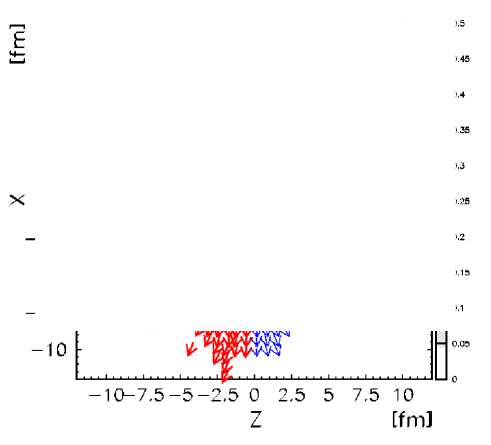
Figure 1: (color online) Net-baryon density for a $Au+Au$ reaction at 8 A GeV, and $b=3$ fm, with an EoS with phase transition at $t=$12 fm/c in the reaction plane with velocity arrows for mid-rapidity ($y<0.5$) fluid elements. Antiflow is indicated by thin, blue arrows, normal flow is indicated by bold red arrows. From ref. [7].

The detailed and quantitative analysis of flow patterns is of vital importance, as these provide the possibly most direct information about the pressure and about the space-time configuration of matter.

The equations of perfect FD are just the local energy and momentum conservation laws, where we assume that the energy-momentum tensor is given by the EoS, in a simple covariant form. The underlying assumption is that the system is in local thermodynamical equilibrium. Thus, the most important input is the EoS, while recent high energy collisions in the QGP domain point at the importance of transport properties, especially of low viscosity.

In the late 70s and early 80s the applicability and relevance of fluid dynamics were frequently questioned. The early suggestions of Mach cone and Mach shock waves, as well as the experiments in the early 70s mentioned above did not uniformly convince the researchers in the field. More detailed and more precise modeling work was needed with new measurable signatures of the collective flow. Apart of the EoS describing the properties of matter in local thermal equilibrium, the importance of transport properties, especially the viscosity and transport processes was recognized very early also.[9, 10, 11]

The other question was what are the most typical, measurable flow phenomena. As most collisions happen at finite impact parameters, in these reactions instead of symmetric Mach cones, a bounce off, side splash or directed flow develops in a well defined azimuthal and polar direction in the reaction plane according to the predictions of the Frankfurt group. [12, 13, 14, 15] This typical flow pattern was also obtained independently in Los Alamos model calculations [16, 17]. Still it had to be shown that the fluid dynamical predictions are significantly different from predictions of random nuclear cascade, without collective flow effects. This was also done in a concerted theoretical effort [18]. The resulting directed flow or bounce off effect could then be observed in different measurable quantities, including two particle and multi-particle correlations, among nucleons and nuclear fragments [12, 13, 14, 15].

As mentioned before, the first comprehensive experimental work that fully confirmed the existence of collective flow and the bounce effect was published in 1984. [4] Shortly after the streamer chamber measurements could also confirm the existence of collective flow, using a sensitive evaluation method developed by Danielewicz and Odyniecz [19]. This method was so sensitive that it could confirm the existence of collective flow even in emulsion experiments of a sample of about 100 events and only a few hundred particles! [20]

In the next decade we learned the basic features of the EoS of hot and compressed nuclear matter, its compressibility. Flow measurements have contributed to the discovery of nuclear liquid-gas phase transition: at the National Superconducting Cyclotron Laboratory at Michigan State University, at energies around 50 MeV/nucleon negative flow was observed as a consequence of the phase transition.

Even more interesting that already at this time transport properties viscosity and Reynolds number of the hot and compressed nuclear matter were studied [21], via energy and mass scaling of collective flow data.

In the 1990s flow measurements continued to develop. With increasing energy the dominance of directed flow decreased, due to the increasing longitudinal momentum component and decreasing collective transverse component of the flow. At the same time the azimuthal asymmetry of collective flow became more dominant and stronger elliptic flow was detected with increasing beam energies. Simultaneously new forms of collective flow parameterizations were introduced, $v_{1},v_{2},v_{3},...$ etc. This parametrization provided some advantages and was more systematic in describing the azimuthal symmetries and asymmetries of the reaction. Still, it led to some side-effects, which complicated the subsequent development.

First of all the longitudinal momentum distribution was not analysed with the same precision and systematic way. This is in part due to the experimental conditions, where at increasing energies the measurement of the particle emission at a larger rapidity range between the projectile rapidity, $y_{P}$, and the target rapidity, $y_{T}$, became increasingly difficult (although recently a similar harmonic expansion in terms of Chebyshev polynomials was also introduced [22]). Due to the experimental constrains this is unfortunately not yet used in experimental analyses.

The other side effect of this development that the symmetry axes of the collision, i.e. the event-by-event direction of the impact parameter vector ($x$-direction) was not performed in all experiments, neither the precise determination of the CM of the participant system, which can fluctuate both in the beam and transverse directions. E.g. in ref. [23] the participant CM. was not determined (which could be done by using the method proposed in ref. [24]) neither in the transverse nor in the longitudinal direction where the fluctuation of the CM. rapidity is much larger. This may have resulted in unexpected artifacts.

These developments and experimental difficulties led to the dominance of the elliptic flow (as well as other even $v_{n}$ studies where an ”Event plane” could be determined by ”cumulative” two particle correlations, without determining the Reaction Plane (i.e. the impact parameter vector’s direction) precisely. This also led to some confusion in analysing flow patterns arising from initial state collision symmetries and from different random fluctuations. We will discuss this problem later in more detail.

The collective flow in form of elliptic flow remained a sensitive signal of the changes in EoS and of all matter properties. It was predicted that the signature of QGP formation and the related softening of the EoS, modifies the $v_{1}$ and $v_{2}$ data and lead to an appearance of the ”third flow component” or ”anti-flow”, [6] which was observed a few years later together with several other signals of QGP formation. In many of these observations the collective flow played important direct or indirect role.

1.2 Causes of the Dominance of Fluid Dynamics

With increasing energies, especially at RHIC, the collective flow effects became increasingly dominant. This was to be expected as the hadron multiplicity grew above 5000 in these reactions, and the matter more and more behaved like a continuum. On the other hand questions of the fundamental stability and the role of dissipation, especially of viscosity gained increasing attention again.

Collective laminar flow is based on momentum correlations among numerous neighboring particles. This requires momentum exchange among neighboring fluid elements. This leads to the reduction of local flow velocity differences, and these differences are dissipated into heat. Such a process is described by the viscosity of the fluid. If viscosity is too small the flow becomes turbulent. If viscosity is too large, dissipation becomes too large and flow patterns characterized by different flow velocities at different locations are dissipated away.

The stability of the flow requires a certain minimum level of viscosity. This stability against turbulent instabilities is characterized by the dimensionless, Reynolds number:

$$Re=l_{1}u_{1}/\nu$$

where $l_{1}$ is the characteristic length scale of the flow pattern, $u_{1}$ is the characteristic flow velocity, $\nu=\eta/\rho$ is the kinetic viscosity, $\eta$ is the shear viscosity, and $\rho$ is the mass (or energy) density.

In an ideal (or perfect) fluid any small perturbation increases and leads to turbulent flow. For stability sufficiently large viscosity and/or heat conductivity are needed!

$$Re\leq 1000-2000$$

Calculations are also stabilized by numerical viscosity! (Even if the equations which are solved are formally describing a perfect fluid with zero viscosity.)

This stability condition is originally applied to mechanical stability, for processes around or above the sound speed. Highly energetic or high temperature phenomena present an additional challenge. Here it was realized recently the decisive role of radiative energy and momentum transfer, thus the application of relativistic fluid dynamics is vital. Thus apart of heavy ion reactions these stability considerations are vital in rocket propulsion, energetic implosions, fission- and fusion reactions, etc.

Numerous recent theoretical studies, especially by D. Molnar [25], U. Heinz [26], et al., estimated the value of viscosity in ultra-relativistic heavy ion reactions at RHIC energies as $\eta\ \approx\ 50-500{\rm MeV/fm}^{2}{\rm c}$ thus $Re\ \approx\ 10-100$. Based on experimental results in the energy range of 50 - 800 MeV/nucleon in the 1980”s using scaling analysis of flow parameters, the Reynolds number was obtained as $Re\approx 7-8$. [21] This was a result for more dilute, and so, more viscous matter.

In both cases $\eta/s\approx 1$ (0.5 - 5). This is a value large enough to keep the flow laminar in Heavy Ion Collisions!

On the other hand the surprising dominance and strength of the collective flow phenomena indicate that the flow is near to perfect in heavy ion reactions. About half of all available energy appears in form of collective flow at and below the transition to QGP (see e.g. [27] Fig. 6). Thus, only a small fraction of energy could be dissipated away, especially as the phase transition itself contributes to dissipation and entropy increase also. Thus, this is almost a paradox, the very strong flow also indicates that the viscosity is small, and so the viscosity must be sufficiently small and sufficiently large at the same time, to satisfy all requirements and observations.

Another comment is relevant here: The collective flow must develop mainly in the quark gluon phase. There are strong indications that hadronization and freeze out are happening simultaneously in heavy ion reactions [28, 29]. This is indicated by the large abundance of multi-strange baryons and by the small freeze out size extracted from two particle correlation data. Finally the scaling of flow with the quark number of observed hadrons also indicates that flow develops mostly in the quark-gluon phase. Thus, the physical features which considerably influence flow phenomena at RHIC energies (like viscosity and EoS), should be primarily the features of QGP!

Since usually the bulk viscosity is small compared to the shear viscosity, the dimensionless ratio of (shear) viscosity to entropy (disorder) $\eta/s$ is a good way to characterize the intrinsic ability of a substance to relax towards equilibrium.

The recent developments address both the EoS and the transport properties of the extreme matter formed in heavy ion reactions. These aspects were addressed recently [30], and a part of the issues discussed here were mentioned at this conference.

In a recent paper Kovtun, Son and Starinets have shown that certain field theories, that are dual to black branes in higher space-time dimensions, have the ratio $\eta/s=1/4\pi$ [31]. Interestingly, this bound is obeyed by ${\cal N}=4$ supersymmetric $SU(N_{c})$ Yang-Mills theory in the large $N_{c}$ limit [32]. They ”speculated” that all substances obeyed this bound, and argue that this is a lower limit especially for such strongly interacting systems where up to now there is no reliable estimate for viscosity, like the QGP. According to the authors: the viscosity of QGP must be lower than that of classical fluids.

Recent advances in the study of the collective flow properties, have a wide spread of directions. Due to the low viscosity of Quark-Gluon plasma near to the phase transition threshold [31, 33], both significant fluctuations may develop [34] and new Global Collective instabilities may occur, as turbulence in peripheral reactions. The precise analysis of these effects would require the experimental separation of these effects as well as the theoretical study of these effects separately, and then their possible interaction and interference in the observables. The necessity of this separation was pointed out recently [35], and we will elaborate this subject in more detail here.

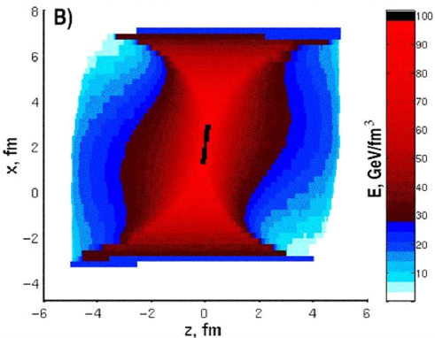
Figure 2: The initial state energy density distribution shown in the Reaction Plane, in the $[x,z]$, plane. This initial state is constructed based on a Glauber model, via fire-streaks, which extend longitudinally. This extension is slowed down by the attractive, chromo-electric, coherent Yang-Mils fields. The resulting string-rope tension is smaller when we have less color charges at the end of the streaks, and this results in a longer streaks and smaller energy density at the top (projectile) and bottom (target) sides. The top and bottom layers move into the opposite directions in the CM frame. The central streaks that stopped stronger, start a 1D Riemann scaling expansion. This initial state, in contrast to many oversimplified ones, conserves energy, momentum, angular momentum, and shows initial vorticity and longitudinal shear. From ref. [36, 37].

Another, recent problem is the formation and study of realistic 3+1D initial states in fully realistic description, without unrealistic simplifying assumptions. Here, Fluctuations and Global Collective flow should also be separated, and the Global Collective initial state model should reflect all symmetries of a heavy ion reaction. This is still not always the case.

In numerous fluid dynamical models, which use the $x,y,\eta,\tau$ coordinates, it is easy to assume uniform longitudinal Bjorken scaling flow, so that $v_{\eta}=0$, and it is done frequently even in 3+1D models, this eliminates immediately the longitudinal shear flow, and the arising vorticity. When the longitudinal momentum distribution is uniform in the transverse plane or if it is symmetric around the collision’s $z$-axis the initial angular momentum is lost, which disables the description of many fundamental phenomena, and also violates the conservation of angular momentum. For a realistic model the longitudinal ends of the initial state (in terms of $z,t$ or $\eta,\tau$), should not exceed the projectile and target rapidities, rather the recoil and the deceleration caused by the other colliding nucleus should be also taken into account. Only a few models satisfy fully, all conservation laws, and we will discuss the construction of realistic initial state configurations for the Global Collective flow component.

There are few realizations where the conservation laws are fully satisfied. The models generating the initial state from a realistic molecular dynamics or cascade model may reach states close to equilibrium, and the smooth average of such states can serve as an realistic 3+1D initial state. One can also construct a good analytic initial state by taking into account of all symmetries and all conserved quantities and their conservation laws. Such an initial state is described in [36, 37] and presented in Fig. 2.

2 Splitting of Global Collective Flow and Fluctuations

The high multiplicities at high energy heavy ion collisions have enabled us to study fluctuations and the distribution of the azimuthal harmonic components. Due to traditional reasons the azimuthal distributions are parametrized in terms of cosine functions and a separate event-by-event fitted Event Plane azimuth, which did not correlate with the Reaction Plane and had nontrivial correlation among the Event Planes of the different harmonic components.

The non-fluctuating Global Collective (background) flow, if the event-by-event center of mass and Reaction Plane are identified, can be written in the form

$$\frac{d^{3}N}{dydp_{t}d\phi}=\frac{1}{2\pi}\frac{d^{2}N}{dydp_{t}}\left[1+2v_{1}(y-y_{CM},p_{t})\cos(\phi-\Psi_{RP})+\right.$$

$$\hskip 128.0374pt\left.2v_{2}(y-y_{CM},p_{t})\cos(2(\phi-\Psi_{RP}))+\cdot\cdot\cdot\ \right]$$ (1)

where $\Psi_{RP}$    and    $y_{CM}$ can be determined experimentally event-by event, as described in [24].

The Fourier components are functions of $p_{t}$ and rapidity $y$. Most data are collected for $v_{2}(y,p_{t})$ at and near CM rapidities, and as function of $p_{t}$ . These data are quite well fitted already by early simple FD models, even by those, which did not calculate the fluid’s dynamics in the $z$ direction, rather these assumed that the longitudinal part of the expansion is described by the Bjorken’s scaling FD model.

Notice that due to fluctuations the event-by event CM fluctuates strongly, in the beam direction $y_{CM}$ fluctuates due to the large rapidity difference between the projectile and target, and due to the event-by event CM fluctuation, also the event-by-event azimuthal angle of the Reaction Plane, $\Psi_{RP}$, will be modified. This second effect was taken into account in ref. [23], without referring to [24], but the stronger longitudinal fluctuations were not studied, and were considered just as ”dipole like initial fluctuations”.

In contrast to the above formulation, fluctuating flow patterns are analysed by using the ansatz

$$\frac{d^{3}N}{dydp_{t}d\phi}=\frac{1}{2\pi}\frac{d^{2}N}{dydp_{t}}\left[1+2v_{1}(y,p_{t})\cos(\phi-\Psi_{1}^{EP})+\right.$$

$$\hskip 128.0374pt\left.2v_{2}(y,p_{t})\cos(2(\phi-\Psi_{2}^{EP}))+\cdot\cdot\cdot\ \right],$$ (2)

which is adequate for exactly central collisions where the Global Collective flow does not lead to azimuthal asymmetries. Here $\Psi_{n}^{EP}$ maximizes $v_{n}(y,p_{t})$ in a rapidity range, and both $\phi$ and $\Psi_{n}^{EP}$ are measured in the laboratory (collider) frame.

If this formulation is used for peripheral collisions the analysis is rather problematic, because patterns arising from Global Collective flow and from fluctuations are getting mixed up. This is actually also true in central collisions with spherical or cylindrical symmetry but there the separation is more subtle, and it does not show up directly in the azimuthal flow harmonics. Still in special model calculations fluctuations in the transverse plane were studied, and Global Collective flow (background flow) was separated from fluctuations [38].

Here we show that the ansatz of flow analysis can be reformulated in a way, which makes the splitting or separation of the Global Collective flow from Fluctuations easier. This can be done based on the final components of given types of symmetries arising from the symmetries of the initial states of peripheral heavy ion collisions. This formulation is also an ortho-normal series expansion for both $\phi$-even and $\phi$-odd functions.

Considering the relation $\cos(\alpha{-}\beta)=\cos\!\alpha\cos\!\beta+\sin\!\alpha\sin\!\beta$, we can write each of the terms of the harmonic expansion into the form

$$v_{n}\cos[n(\phi-\Psi_{n}^{EP})]=v_{n}\cos(n\Psi_{n}^{EP})\ \cos(n\phi)+v_{n}\sin(n\Psi_{n}^{EP})\ \sin(n\phi).$$

If we consider that the unique reaction plane, $\Psi_{RP}$ can be determined event-by-event experimentally also [24], we can introduce $\Phi_{n}^{EP}\equiv\Psi_{n}^{EP}-\Psi_{RP}$ and $\phi^{\prime}\equiv\phi-\Psi_{RP}$, so that from these data we get $\Psi_{n}^{EP}=\Phi_{n}^{EP}+\Psi_{RP}$. Here $\phi^{\prime}$ is the azimuth angle with respect to the Reaction Plane. Now we can also define the new flow harmonic coefficients by

$${}^{c}v^{\prime}_{n}\equiv v_{n}\cos(n(\Psi_{n}^{EP}))\ \ {\rm and}\ \ ^{s}v^{\prime}_{n}\equiv v_{n}\sin(n(\Psi_{n}^{EP}))\ ,$$

and we get for the terms of the harmonic expansion

$$v_{n}\cos[n(\phi-\Psi_{n}^{EP})]=\ v_{n}\cos[n(\phi^{\prime}-\Phi_{n}^{EP})]\ =\ ^{c}\!v^{\prime}_{n}\cos(n\phi^{\prime})+\ ^{s}\!v^{\prime}_{n}\sin(n\phi^{\prime}).\ \$$ (3)

Thus we have reformulated the azimuthal angle harmonic expansion, which was given originally in terms of cosines and Event Plane angles for each harmonic component, to both sines and cosines in the Reaction Plane as reference plane and the corresponding new coefficients ${}^{c}\!v^{\prime}_{n}=^{c}\!v^{\prime}_{n}(y-y_{CM},p_{t})$ and ${}^{s}\!v^{\prime}_{n}=^{s}\!v^{\prime}_{n}(y-y_{CM},p_{t})$. These can be obtained from the measured data, $v_{n}$, $\Psi_{n}^{EP}$, $\Psi_{RP}$ and $y_{CM}$ directly.

As the Global Collective flow in the configuration space has to be $\pm y$ symmetric, all the coefficients of the $\sin(n\phi^{\prime})$ terms should vanish: ${}^{s}\!v^{\prime}_{n}=0$. These symmetry properties provide a possibility to separate the fluctuating and the global flow (background flow) components.

This form has the advantage that in peripheral collisions the Global Collective (not fluctuating) flow component, ${}^{c}\!v^{\prime}_{n}$ for odd harmonics have to be odd functions of $(y-y_{CM})$, while for even harmonic components have to be even function of rapidity, $(y-y_{CM})$. Let us now introduce the rapidity variable ${\bf y}\equiv y-y_{CM}$.

When the new coefficients ${}^{c}\!v^{\prime}_{n}=\ ^{c}\!v^{\prime}_{n}({\bf y},p_{t})$ and ${}^{s}\!v^{\prime}_{n}=\ ^{s}\!v^{\prime}_{n}({\bf y},p_{t})$, are constructed, we can conclude that ${}^{s}\!v^{\prime}_{n}$ can be due to fluctuations only. Furthermore for the Global Collective flow, ${}^{c}\!v^{\prime}_{n}({\bf y},p_{t})$ must be an even (odd) function of ${\bf y}$ for even (odd) harmonic coefficients. Due to the fluctuations this is usually not satisfied and one has to construct the even (odd) combinations from the measured data. These represent then the Global Collective component, while the odd (even) combination will represent the Fluctuating component. We obtain the Fluctuating component by subtracting the Global Collective component from the Total (mixed) flow harmonic term:

$$v_{n\frac{even}{odd}}^{Coll.}\cos[n(\phi-\Psi_{n}^{EP})] = \frac{1}{2}\left[{}^{c}\!v^{\prime}_{n}({\bf y},p_{t})\pm\ ^{c}\!v^{\prime}_{n}(-{\bf y},p_{t})\right]\cos(n\phi^{\prime})$$ (4)

$$v_{n\frac{even}{odd}}^{Fluct.}\cos[n(\phi-\Psi_{n}^{EP})] = \frac{1}{2}\left[{}^{c}\!v^{\prime}_{n}({\bf y},p_{t})\mp\ ^{c}\!v^{\prime}_{n}(-{\bf y},p_{t})\right]\cos(n\phi^{\prime})$$ (5)

$$\phantom{\frac{1}{2}\left[\right.}+^{s}\!v^{\prime}_{n}({\bf y},p_{t})\ \sin(n\phi^{\prime})$$

This separation provides an upper limit for the magnitude of the Global Flow component, because the fluctuations may in some events show the same symmetries as the Global Collective flow. On the other hand, for the Fluctuating component, ${}^{s}\!v^{\prime}_{n}$, provides an upper limit, because this component cannot be caused by the Global Collective flow. A last essential guidance may be given by the conditions that the fluctuations must have the same magnitude for sine and cosine components as well as for odd and even rapidity components.

The evaluation of experimental results this way may provide a better insight into both types of flow patterns. Furthermore, these can also help judgements on theoretical model results, and the theoretical assumptions regarding the initial states.

Other experimental methods, like two particle correlations [39] or polarization measurements [40], may take advantage of this splitting of flow pattern components also.

2.1 Negative $v_{1}(p_{t})$

The Global Collective directed flow, $v_{1}$, becomes negative due to the softening of the EoS in Quark-gluon Plasma [6, 7]. This shows up at CERN SPS, RHIC and LHC energies, and was first predicted in fluid dynamical calculations in 1994, see [27] Fig. 8, and in 1995 [41]. The softening effected $v_{2}$ also as predicted e.g. in RQMD calculations [42]. This softening makes $v_{1}({\bf y})$ negative at small positive rapidities, and thus at the these rapidities $v_{1}({\bf y},p_{t})$ will also be negative. The rapidity integrated $v_{1}(p_{t})$ at the same time should vanish as the Collective directed flow, $v_{1}$, should be an odd function of rapidity. Furthermore in any case due to transverse momentum conservation $\langle v_{1}(p_{t})\rangle=0$ [43]. In Global Collective flow models, e.g. in fluid dynamical models without random fluctuations, the integrated $v_{1}(p_{t})$ should vanish, while the symmetrized $v^{S}_{1}(p_{t})$ [44] can be finite and usually still positive.

On the other hand, recent measurements yield negative $v^{S}_{1}(p_{t})$ values at low rapidities, $p_{t}<1.2-1.5$Gev/c [45, 46, 23]. The same is observed in model calculations both in fluid dynamics [47] and in molecular dynamics [43] with random fluctuating initial conditions. This is not unexpected.

Still there is a problem. When the Global Collective flow and Fluctuating flow are not separated and the CM is not identified the contributions of Events with different unidentified CM points can lead to negative $v^{S}_{1}(p_{t})$ also, as it can be clearly seen from eqs. (2) and (3) of ref. [44]. This is a consequence of not identifying the EbE CM of the participant system, which is also fluctuating, but this fluctuation has different physical grounds then e.g. critical fluctuations arising from the phase transition.

The main cause of the longitudinal CM fluctuations is that the target and projectile spectators must not be identical and so, their momenta are also different. At the same time this fluctuation does not influence the nonlinear dynamical evolution of the participant system, which arises from the random initial configuration, the critical dynamics, and the randomness in the freeze out process.

The interference of the global collective and the fluctuating dynamics is well represented by the detailed results in ref. [45].

In order to extract the physical features of the QGP based on the observed fluctuations it is of utmost importance to separate the Global Collective flow components from the Fluctuating flow components.

Gyulassy et al. [48] claim that recent low $p_{t}<2$ GeV azimuthal correlation data from the beam energy scan (BES) and D+Au at RHIC/BNL and the especially the surprising low $p_{t}$ azimuthal $v_{n}(p_{t})$ in p+Pb at LHC challenge long held assumptions about the necessity of perfect fluidity (minimal viscosity to entropy, $~{}1/4\pi$) to account for azimuthal asymmetric ”flow” patterns in A+A. The work discusses basic pQCD interference phenomena from beam jet color antenna arrays that may help unravel these puzzles without requiring perfect fluid hydrodynamic or CGC Glasma diagrams, but only LO Feynmann diagrams.

First we have to comment that comparing p+p and peripheral Pb+Pb data is not trivial, as most of the time equal multiplicity collision are compared, where the geometry of the two types of collisions is very different.

Furthermore the Global Flow and the Fluctuating Flow dynamics are not analyzed separately, thus it is unclear what these comparisons refer to.

Finally the $v_{1}$ measurements, which are separately mentioned in ref. [48], their methods, and the results are problematic and therefore avoided in most experimental and theoretical publications. As a matter of fact similar problems appear in case of all odd flow harmonics also, but here the fluctuating component is dominant so the effect of separating the background Global Collective flow component does not cause a large difference.

$v_{1}(y)$ observations show a central antiflow slope, $\partial v_{1}(y)/\partial y$, which is gradually decreasing with increasing beam energy [23]:

$$\frac{\partial v_{1}(y)_{odd}}{\partial y}=\left\{\begin{array}[]{llrl}-1.25\%&{\rm for}&62.4\ {\rm GeV}&{\rm(STAR)}\\ -0.41\%&{\rm for}&200.0\ {\rm GeV}&{\rm(STAR)}\\ -0.15\%&{\rm for}&2760.0\ {\rm GeV}&{\rm(ALICE)}\\ \end{array}\right.$$

This decrease is partly due to the smaller increase of the pressure and the caused transverse motion. In addition the forward rotation of the antiflow peak with increasing angular momentum [44] leads to a decrease also as the peak approaches the turnover point where the antiflow peak would turn over to directed flow. The non-identification of the participant system’s CM leads to a strong smoothing and decrease of the $v_{1}(y)$ peak [44], but the experimental result [23] indicates that the peak is still in the antiflow direction, and the predicted turn over to directed flow did not happen. This shows that the rotation at the present 2.76 TeV energy is not sufficient to reach the turnover point before freeze-out. However, at the double beam energy with double angular momentum the turnover may take place.

Returning the alternative suggestion of Gyulassy et al. [48] of creating azimuthal asymmetry in microscopic processes in LO Feynmann diagrams, these may have a role in p+p or eventually in p+A collisions, however, as discussed above the azimuthal and longitudinal dynamics is strongly connected in A+A collisions with substantial Global Collective flow processes. In Pb+Pb collisions there is to long a distance between the sources/minijets, which according to [48] shall produce the $v_{2}$ (and higher even) flow harmonics from their Gluon correlation/interference. The modifications are independent of pseudorapidity, thus will have minor or no contributions to odd flow harmonics. In Pb+Pb it is hardly feasible that these processes will be correlated with the Reaction Plane and the participant CM, thus only the Fluctuating component will be influenced by these azimuthal correlations of microscopic origin.

Reference [48] points out the negative $v_{1}(p_{t})$ at low transverse momenta. We discussed this effect in this subsection in general by comparing the Global Collective and Fluctuation contributions, and the effect of non-identification of the participant CM. The processes discussed in [48] can thus contribute to the Fluctuating component of the flow. This, however has many other origins: Initial configuration fluctuations, Langevin fluctuations in critical dynamics, fluctuations arising from the hadronization and freeze out, etc. The separate analysis of these numerous processes is particularly difficult experimentally. The reasonable first step of such an analysis is to extract the non-Fluctuating global collective flow, and in the next step one may distinguish the different origins of the fluctuating flow.

We conclude that ref. [48] will not contribute to the study of the negative $v_{1}(p_{t})$ at low transverse momenta, other than the suggested processes contribute to the fluctuation flow components just as the other causes of fluctuation. With increasing system size the role and observability of these microscopic processes must decrease.

3 The Initial State

As we have shown in the introduction the Initial State can be constructed in a way such that all conservations laws are satisfied, and no simplifying assumptions are used, which would violate the conservation laws. In addition there are other principles like causality which should also be satisfied by the initial state.

A frequent simplification in $x,y,\eta,\tau$ coordinates, is to assume uniform longitudinal Bjorken scaling flow (this leads to a simple separable initial state distribution function), and in order to satisfy the angular momentum conservation at different transverse points the energy density or mass distribution is made such that on the projectile side a substantial part of the mass is at rapidities exceeding the target and projectile rapidity [49, 50, 51]. In most cases this leads to acausal distributions where part of the matter is situated beyond the target and projectile rapidities. This acausality is corrected by Karpenko et al. [52] by cutting the distributions at the target and projectile rapidities. Still the attractive chromo field is not taken into account in this approach, which would limit the initial limiting rapidities by up to 2.5 units of smaller rapidities on each side [53, 54, 55].

Furthermore, the Bjorken scaling flow approach eliminates any possibility for initial shear flow and vorticity, which is a dominant source of simple flow patterns and of strong and visible instabilities in classical physics, like rotation and turbulent Kelvin Helmholtz Instability. Apart of the semi-analytic initial state model mentioned in the introduction other initial state models exist, which satisfy all conditions of a realistic initial state. First of all initial state molecular dynamics and multi-particle cascade models which satisfy all conservation laws, boundary conditions and causality, will provide realistic Global Collective initial state as the average of many such realistic events. Also, analytic models can be constructed based on these principles, which are different from the one mentioned in the introduction.

The initial uniform Bjorken scaling flow is maintained during the fluid dynamical development, so that the lack of shear-flow persists in these solutions. It follows that no viscous dissipation takes place in the longitudinal direction, which makes the model configurations anisotropic and not very reliable in this model configurations.

Initial State (IS) models are frequently based on molecular dynamics type or string models like, uRQMD, QGSM or PACIAE, where the interacting gluon fields play a secondary role. Since 2001, recent IS models take into consideration strong gluon fields arising from the Color-glass Condensate (CGC) [56], which lead to more compact and longitudinally less extended initial spatial configurations. A few models, [36, 37, 55] have taken such a collective, attractive classical Yang-Mills (CYM) flux tube picture into account even before [57]. More recent models, e.g. IP-Sat and IP-Glasma [58, 59] use the CGC Glasma flux tube picture. The resulting more compact initial state leads to stronger equilibration and enhances collective dynamics, including rotation. While the earlier models [36, 37, 55] did not take into account random fluctuations the more recent ones mostly do, using the MC-Glauber or similar schemes. This Scheme if adequately used leads to large conserved angular momentum and shear flow [60], although in some applications the shear flow and the angular momentum are neglected and then the collective flow in the odd harmonics is eliminated.

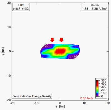
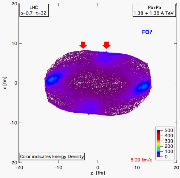
Figure 3: The rotation during the fluid dynamical evolution is indicated by the red arrows pointing to the initial central and corner points on the surface. The motion of these points shows the rotation of the system. The fluid dynamical initial state is preceded by an pre-equilibrium Yang-Mills longitudinal field theoretical model, which took 6.25 fm/c. Thus after 2.00 fm/c fluid dynamical evolution the length of the matter is 8.25 fm (l.h.s). The configuration on the r.h.s. is at 8 fm/c fluid dynamical evolution, which is 14.25 fm/c after the initial touch of the two nuclei. This is just after the estimated freeze out time of 10-12 fm/c. Based on ref. [44] and [30].

4 New Global Collective Flow Patterns

As mentioned in the introduction, in collisions of finite impact parameter at high energies we have a large angular momentum which can be as high as J = $10^{6}$ $\hbar$ at LHC. The angular momentum is conserved, but due to the explosive expansion of the system the angular velocity of the participant system is rapidly decreasing, thus the local rotation, the vorticity, decreases with time. It depends on the balance between the expansion and the angular momentum if the rotation will manifest itself in observable quantities at the Freeze out.

Due to the widespread use of the uniform longitudinal Bjorken scaling flow in the initial condition, the rotation did not occur in fluid dynamical model calculations, and it was studied only recently. First it was noticed in ref. [44], see Fig. 3.

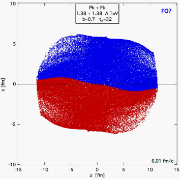
Figure 4: The fluid dynamical development of the shape of the dividing surface between the initial top and bottom halves of the dense matter. The developing non-linear, turbulent wave is the initial stage of a Kelvin Helmholtz Instability. The fluid dynamical initial state indicated by 0.00 fm/c is preceded by an pre-equilibrium Yang-Mills longitudinal field theoretical model, which took 6.25 fm/c indicated by the length of the dense matter. The configuration on the r.h.s. is at 6 fm/c fluid dynamical evolution, which is 12.25 fm/c after the initial touch of the two nuclei. This is just around the estimated freeze out time of 10-12 fm/c. Based on ref. [61] and [30].

This rotation acts against the 3rd flow component or antiflow, and may decrease the measured directed flow, or even reverses the direction from antiflow to directed flow. According the calculations [44] the $v_{1}$ was expected to peak at positive rapidities, but this prediction is strongly dependent on the competition between the rotation and the expansion. The small amplitude of $v_{1}$ is difficult to identify in the strongly fluctuating background, without identifying the event-by-event center of mass and Reaction Plane.

The fluid dynamical calculations with the same method showed for the first time the possibility of the turbulent Kelvin Helmholtz Instability [61]. See Fig. 4. Stability estimates confirmed the possibility of the occurrence if this instability, which could also be obtained in a simple analytic model [62].

Interestingly in a recent work the holographic method is used to study features similar to the KHI, which appear in gauge-gravity duality. Here the dual rotating black holes are more sensitive to the asymptotic geometry than shearing black holes, because topologically spherical AdS black holes differ from their planar counterparts [63].

5 Detecting the New Flow Patterns via Polarization

The rotation and the turbulence have a small effect on the directed flow, which is weak at RHIC and LHC energies anyway, so alternative ways of detection should be considered.

The angular momentum in case of distributed shear flow, shows up in local vorticity. The simplest classical expression of vorticity in the reaction plane, [x-z], is defined as:

$$\omega_{y}\ \equiv\ \omega_{xz}\ \equiv\ -\omega_{zx}\equiv\ \frac{1}{2}(\partial_{z}v_{x}-\partial_{x}v_{z})$$ (6)

where the $x,\ y,\ z$ components of the 3-velocity $v$ are denoted by $v_{x},\ v_{y},\ v_{z}$ respectively. In 3-dimensional space the vorticity can be defined as

$$\mbox{\boldmath$\omega$}\equiv\frac{1}{2}{\bf rot}\ \mbox{\boldmath$v$}=\frac{1}{2}\,\nabla\times\mbox{\boldmath$v$}\,$$ (7)

For the relativistic case, the vorticity tensor, $\omega^{\mu}_{\nu}$ is defined as

$$\omega^{\mu}_{\nu}\equiv\frac{1}{2}(\nabla_{\nu}u^{\mu}-\nabla^{\mu}u_{\nu}),$$ (8)

where for any four vector $q^{\mu}$ the quantity $\nabla_{\alpha}q^{\mu}\equiv\Delta^{\beta}_{\alpha}\,\partial_{\beta}q^{\mu}=\Delta^{\beta}_{\alpha}\,q^{\mu}_{,\beta}$ and $\Delta^{\mu\nu}\equiv g^{\mu\nu}-u^{\mu}u^{\nu}$. The relativistic generalization of vorticity leads to an increase of the magnitude of vorticity [64].

The local vorticity is decreasing with the expansion, but it is still significant at Freeze out in peripheral collisions due to the huge initial angular momentum. the local vorticity reaches 3 c/fm in the reaction plane [64], which is more than an order of magnitude larger than the vorticity in the transverse plane arising from random fluctuations [65]. Other similar collective chiral vortaic effects were predicted for lower energies in ref. [66].

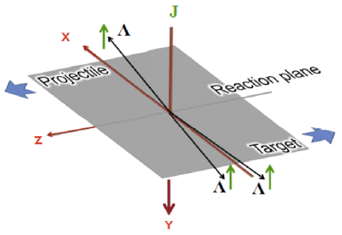
Figure 5: The $[x,z]$, Reaction Plane where the direction of the Projectile and Target matter is indicated. The arising angular momentum, $J$, points into the $-y$ direction. When the event-by-event center of mass and the reaction plane is identified this angular momentum is divided between orbital rotation and polarization or spin. The polarization is transverse to the motion of the $\Lambda$ and $\bar{\Lambda}$ particles and has the same direction as the angular momentum, $J$. Thus, this polarization may be detected in $\Lambda$ and $\bar{\Lambda}$ particles, which are emitted into the $\pm x$ directions. From [40].

This vorticity may lead to two other measurable consequences. According to the equipartition principle for different degrees of freedom carrying the same amount of energy the same applies for angular momentum. Here the local orbital rotation and the spin of the particles may equilibrate with each other. If equilibrium is reached by freeze out the final polarization should have the same direction and magnitude as the local vorticity. Interestingly, high temperature acts against polarization so the polarization is governed by the so called thermal vorticity, where instead of the four velocity, $u^{\mu}$, the inverse temperature four-vector,

$$\beta\,^{\mu}(x)=\frac{u\,^{\mu}(x)}{T(x)}\ ,$$

is used to determine the thermal vorticity [40]. If $\beta\,^{\mu}$ is measured in units of $\hbar$ the thermal vorticity becomes dimensionless. For the polarization studies it is of utmost importance to identify the proper global directions in a collision event-by event. See Fig. 5.

Without identifying the center of mass rapidity, the Reaction Plane, and the Projectile and target side of the reaction plane the detection of the angular momentum and polarization is not possible and earlier measurement at RHIC, where all azimuth angles were averaged over, gave results where the measured polarization was consistent with zero.

Figure 6: The thermal vorticity of the matter arising from a fluid dynamical calculation for two different beam energies. The thermal vorticity is inversely proportional with the temperature, which is increasing faster than the local vorticity with increasing beam energy. Thus the thermal vorticity at RHIC is larger. Also the side regions are cooler and this also increases the thermal vorticity, which enhances the polarization in due to equipartition. Based on ref. [40] and [30].

The $\Lambda$ particle is well suited for measuring its polarization because its dominant decay mode is $\Lambda\longrightarrow p\,\pi^{-}$ and the proton is emitted in the direction of polarization. Notice that due to the thermal and fluid mechanical equilibration process the polarization of $\Lambda$s and $\bar{\Lambda}$s are the same. This distinguishes the process from electro-magnetic polarization mechanisms.

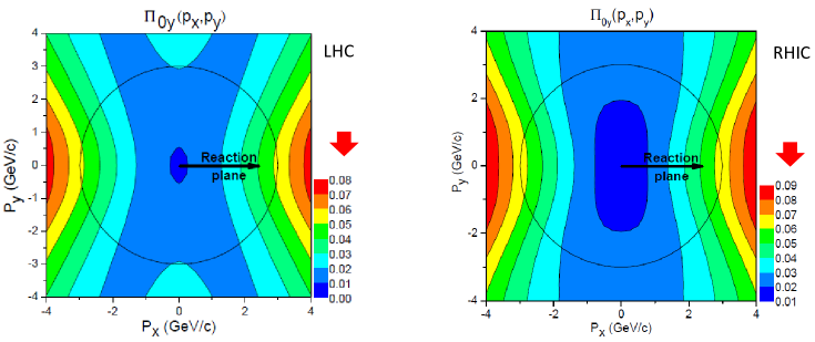
Figure 7: The polarization of the $\Lambda$ and $\bar{\Lambda}$ particles observed in different directions and at different transverse momenta in the transverse, $[x,y]$ plane at the event-by-event CM rapidity for RHIC and LHC energies. Significant polarization can be measured for particles at larger momenta, $p_{t}\geq 3$ GeV/c, in the $\pm p_{x}$ directions. Based on ref. [40] and [30].

The thermal vorticity projected to the Reaction Plane is shown in Fig. 6. The thermal vorticity is more pronounced than the standard vorticity, at the external edges of the matter. where the temperature is lower. The thermal vorticity is somewhat larger at RHIC, where the amount of data and the available detector acceptance are larger.

The resulting polarization is shown in Fig. 7. Thus for this measurement the determination of the proper directions of the collision axes is vital. The polarization should be measured for $\Lambda$s emitted into the $\pm x$ directions, which will then be polarized in the $-y$ direction.

This thermal and fluid mechanical polarization would not exist if the source, the participant system in heavy ion reactions would not have a significant vorticity. This is realized in peripheral heavy ion reactions, which have high initial angular momentum. Unfortunately, even some 3+1D fluid dynamical calculations assume oversimplified initial states where initial shear and vorticity vanishes and these are not able to show these effects.

6 Detecting the New Flow Patterns via Two Particle Correlations

The detection described in the previous section 5, was sensitive to the local vorticity. Two particle correlation measurements are sensitive to the integrated emission from the freeze out space-time zone, the so called ”homogeneity” region, where the dominant emission is directed toward the detection, i.e. in the (out)-direction.

Recently we proposed the Differential Hanbury Brown and Twiss method to study the rotation of the source via two particle correlations [39, 67]. The method is based on a simple observation, if we have a spherically symmetric or cylindrically symmetric source with an rotation axis, or any source which is left/right symmetric with respect to a given ”out-direction”, of momentum $k$, then we can construct from the usual two particle correlation function with momenta $p_{1}=k+q/2$ and $p_{2}=k-q/2$:

$$C(k,q)=\frac{P_{2}(k+q/2,k-q/2)}{P_{1}(k+q/2)P_{1}(k-q/2)}.$$ (9)

This correlation function does not depend on the direction of $k$ for static, spherically or cylindrically symmetric sources, and gives the same value for two, $k_{+}$ and $k_{-}$ momentum vectors which are tilted to left/right with the same tilt angle in case of a left/right symmetric source with respect to $k$. Even if the source is not static but has local motion with local velocities, the correlation functions have the same value if the velocity of motion is in the radial, i.e. points in the local out-direction.

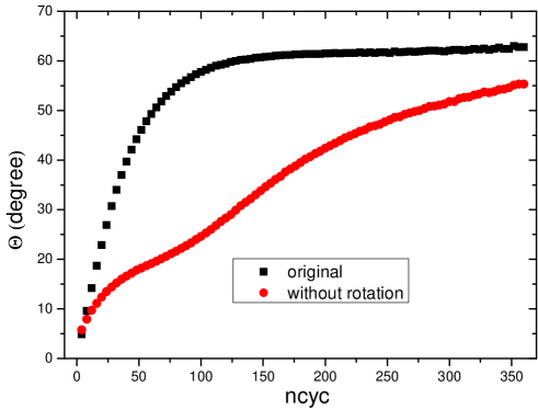
Figure 8: The change of the flow angle with time in a Pb+Pb reaction at $\sqrt{s_{NN}}=2.76$TeV and $b=0.7\,b_{max}$, for the flow tensor for the original flow evolution (black points), while the flow angle development of the flow tensor where the rotational component of the velocity was removed is also shown (red dots). The DCF was evaluated and presented at the time-step, $ncyc=84$ (corresponding to $t=3.56$fm/c), where the flow angle of the rotation-less flow tensor is 22.2 degrees. From [30].

On the other hand this is not true if the local velocities have a ”side” component, i.e. when the source is rotating. This can be tested by the introduction of the Differential Correlation function, $\Delta C(k,q)$, which is defined as

$$\Delta C(k,q)\equiv C(k_{+},q_{out})-C(k_{-},q_{out}).$$ (10)

Now let us assume that the rotation axis is the $y$-axis, the momentum vector $k$, points into the $x$ direction, and the tilted vectors are $k_{+x}=k_{-x}$ and $k_{+z}=-k_{-z}$. In a heavy ion reaction $z$ could be the beam direction and the $x,z$ plane is the reaction plane. E.g. for central collisions or spherical expansion, $\Delta C(k,q)$ would vanish! It would become finite if the rotation introduces an asymmetry.

We have studied the differential $\Delta C(k,q)$ -function, and for symmetric sources its amplitude is increasing with the speed of rotation [67], as expected.

For realistic heavy ion collision studies we used the same PICR fluid dynamical code as in the previous examples. The Global Collective flow shows the same symmetry features, as described above. At peripheral collisions the shape of the emitting source can be approximated with a three axis ellipsoid, and different methods exist to characterize the shape and the directions of the axes. A traditional method is the Global Flow Tensor analysis, which dates back to the 1980s. The main tilt axis of the emission is different with, and without rotation, See Fig. 8.

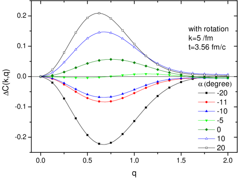
Figure 9: The Differential Correlation Function (DCF) at average pion wavenumber, $k=5/$fm and fluid dynamical evolution time, $t=3.56$fm/c, as a function of the functions of momentum difference in the ”out” direction $q$ (in units of 1/fm). The DCF is evaluated in a frame rotated in the reaction plane, in the CM system by angle $\alpha$. The figure shows the result where the rotation component of the velocity field is not removed with a minimum at $\alpha=-5$ degrees . In contrast the DCF shows a minimum in its integrated value over $q$, for $\alpha=-11$ degrees when the rotation component of the velocity is removed [30]. The shape of the DCF changes characteristically with the angle $\alpha$. The ”rotation-less” configuration is constructed in the fluid dynamical model, where the $\alpha=-11$ degree symmetry angle is found. Unfortunately this is not possible experimentally, so the direction of the symmetry axes should be found with other methods, like global flow analysis and/or azimuthal HBT analysis.

The correlation function for the original fluid dynamical DCF with the rotation included (Fig. 9) is different from the one obtained from the rotation-less configuration (see Fig. 4 of ref. [39]. At the reference frame angle corresponding to the symmetry angle of the rotation-less system, $\alpha=-11$ degrees, the correlation function is distinctly different from the rotation-less one and has a minimum of $-0.085$ at $q=0.63/$fm [39]. Unfortunately this is not possible experimentally, so the direction of the symmetry axes should be found with other methods, like global flow analysis and/or azimuthal HBT analysis.

To study the dependence on the angular momentum the same study was for lower angular momentum also, i.e. for a lower (RHIC) energy Au+Au collisions at the same impact parameter and time. We identified the angle where the rotation-less DCF was minimal, which was $\alpha=-8$ degrees, less than the deflection at higher angular momentum. The original, rotating configuration was then analyzed at this deflection angle, and a minimum of $-0.046$ appears at $q=0.76/$fm. Thus, the magnitude of the DCF at the angle of the symmetry axis increased by nearly a factor of two.

Thus, the method is straightforward for symmetric emission objects, while for a general Global Collective Flow pattern one has to extract the shape symmetry axis with other methods. There are several methods for this task, and it takes some experimental tests, which of these methods are the most adequate for the task.

7 Conclusions

Following the introduction of early flow studies the importance of splitting flow fluctuations from Global Collective Flow was discussed and this separation was presented. Such a separation will enable the separate study the Global Collective flow component, which includes novel new features not studied up to now, including rotation, turbulence, and Kelvin Helmholtz Instability. As the measurement of directed flow is difficult due to its decreasing amplitude at increasing beam energies, alternative detection methods are presented, which are more sensitive to these processes.

We are looking forward that these new phenomena with the help of the suggested methods will open new ways of studying the Quark-gluon Plasma. Especially the transport properties are the key features, as some of the new phenomena, like turbulence and the Kelvin Helmholtz Instability occur only in case of low viscosity.

References

References

-
[1]
Scheid W, Müller H and Greiner W 1974
Phys. Rev. Lett. 32 741
Scheid W, Ligensa R and Greiner W 1968 Phys. Rev. Lett. 21 1479
Scheid W and Greiner W 1969 Z. Phys. 226 364 - [2] Baumgardt H et al 1975 Z. Phys. A 273 359
- [3] Chapline G F, Johnson M H, Teller E and Weiss M S 1973 Phys. Rev. D 8 135
- [4] Gustafsson H Å , Gutbrod H H et al 1984 Phys. Rev. Lett. 52 1590
- [5] Csernai L P 1994 Introdiction to Relativistic Heavy Ion Collisions John Wiley & Sons, Chichester
- [6] Csernai L P and Röhrich D 1999 Phys. Lett. B 458 454
- [7] Brachmann J, Soff S, Dumitru A, Söcker H, Maruhn J A, Greiner W, Bravina L V and Rischke D H 2000 Phys. Rev. C 61, 024909
- [8] Snellings R J M, Sorge H, Voloshin A A, Wang F Q and Xu N 2000 Phys. Rev. Lett. 84 2803; arXiv: nucl-ex/9908001
- [9] Csernai L P and Barz H W 1980 Z. Phys. A 296 173
- [10] Buchwald G, Csernai L P, Maruhn J, Greiner W and Stöcker H 1981 Phys. Rev. C 24 135
- [11] Csernai L P, Lovas I, Maruhn J, Rosenhauer A, Zimányi J, Greiner W 1982 Phys. Rev. C 26 149
- [12] Csernai L P and Greiner W 1981 Phys. Lett. B 99 85
- [13] Stöcker H, Csernai L P, Graebner G, Buchwald G, Kruse H, Cusson R Y, Maruhn J and Greiner W 1982 Phys. Rev. C 25 1873
- [14] Csernai L P, Greiner W, Stöcker H, Tanihata I, Nagamiya S, Knoll J 1982 Phys. Rev. C 25 2482
- [15] Barz H W, Csernai L P and Greiner W 1982 Phys. Rev. C 26 740
- [16] Amsden A A et al 1977 Phys. Rev. C 15 2059
- [17] Amsden A A et al 1975 Phys. Rev. Lett. 35 905
- [18] Stöcker H, Riedel C, Yariv Y, Csernai L P, Buchwald G, Graebner G, Maruhn J, Greiner W, Frankel K, Gyulassy M, Schürmann B, Westfall G, Stevenson J D, Nix J R and Strottmann D 1981 Phys. Rev. Lett. 47 1807
- [19] Danielewicz P and Odyniecz G 1985 Phys. Lett. B 157 146
- [20] Csernai L P, Freier P, Mevissen J, Nguyen H and Waters L 1986 Phys. Rev. C 34 1270.
- [21] Bonasera A and Csernai L P 1987 Phys. Rev. Lett. 59 630; Bonasera A, Csernai L P and Schürmann B 1988 Nucl. Phys. A 476 159
- [22] Bzdak A and Teaney D 2013 Phys. Rev. C 87, 024906
- [23] Abeleev B et al, (ALICE Collaboration) 2013 Phys. Rev. Lett. 111, 232302
- [24] Csernai L P, Eyyubova G and Magas V K 2012 Phys. Rev. C 86 024912
- [25] Molnar D and Huovinen P 2008 J. Phys. G 35 104125
- [26] Song H C and Heinz U 2008 Phys. Lett. B 658 279; Phys. Rev. C 77 064901
- [27] Bravina L, Csernai L P, Lévai P and Strottman D 1994 Phys. Rev. C 50 2161
- [28] Csörgő T and Csernai LP 1994 Phys. Lett. B 333 494; arXiv: hep-ph/9406365
- [29] Csernai LP and Mishustin IN 1995 Phys. Rev. Lett. 74 5005
- [30] Csernai L P and Wang D J 2014 - invited plenary talk at the - Int. Conf. on New Frontiers in Physics, ICNFP2013, (Kolymbari, Greece, 28 Aug. - 5 Sept., 2013) EPJ Web of Conferences, 71 00029
- [31] Kovtun P K, Son D T, Starinets A O 2005 Phys. Rev. Lett. 94, 111601
- [32] Buchel A, Liu J T and Starinets A O 2005 Nucl. Phys. B 707 56
- [33] Csernai L P, Kapusta J I and McLerran L D 2006 Phys. Rev. Lett 97 152303
-
[34]
Kapusta J I, Mueller B and Stephanov M 2013
Nucl. Phys. A 904-905 499c
Kapusta J I, Mueller B and Stephanov M 2012 Phys. Rev. C 85 054906 - [35] Csernai L P 2014 - invited talk at the - (Int. Nuclear Physics Conference, Firenze, Italy, June 2-7, 2013) EPJ Web of Conferences, 66 04007
- [36] Magas V K, Csernai L P and Strottman D D 2001 Phys. Rev. C 64 014901
- [37] Magas V K, Csernai L P and Strottman D D 2002 Nucl. Phys. A 712 167
- [38] Floerchinger S and Wiedemann U A 2013 Phys. Rev. C 89 034914
- [39] Csernai L P, Velle S and Wang DJ 2014 Phys. Rev. C 89 034916
- [40] Becattini F, Csernai L P and Wang D J 2013 Phys. Rev. C 88 034905
- [41] Rischke DH, Pürsün Y, Maruhn JA, Stöcker H and Greiner W 1995 Heavy Ion Physics 1 309
- [42] Sorge H 1999 Phys. Rev. Lett 82 2048
- [43] Zabrodin E E, Fuchs C, Bravina LV and Faessler A 2001 Phys. Rev. C 63 034902, arXiv: nucl-th/0006056
- [44] Csernai L P, Magas V K, Stöcker H and D.D. Strottman 2011 Phys. Rev. C 84 024914
-
[45]
Jia J et al (ATLAS Collaboration) 2012
J Phys. Conf. Ser. 389 012013
Jia J, Radhakrishnan S and Mohapatra S 2013 J. Phys. G: Nucl. Part. Phys. 40 105108 - [46] Aamodt K et al (ALICE Collaboration) 2012 Phys. Lett. B 708 249
- [47] Gale C, Jeon S, Schenke B, Tribedy P and Venugopalan R 2013 Phys. Rev. Lett. 110 012302; arXiv:1209.6330 [nucl-th]
- [48] Gyulassy M, Levai P, Vitev I and Biro T 2014 Int. Conf. QM14, Darmstadt, Germany, May 21-25, 2014; arXiv: 1405.7825 [hep-ph]
- [49] Schenke B, Jeon S Y and Gale C 2010 Phys. Rev. C 82 014903
- [50] Bozek P and Wyskiel I 2010 Phys. Rev. C 81 054902
- [51] Adil A and Gyulassy M 2005 Phys. Rev. C 72 034907
- [52] Karpenko Iu, Huovinen P and Bleicher M 2013 arXiv: 1312.4160v1[nucl-th]
- [53] Csernai L P and Kapusta J I 1984 Phys. Rev. D 29 2664
- [54] Csernai L P and Kapusta J I 1985 Phys. Rev. D 31 2795
- [55] Mishustin I N and Kapusta J I 2002 Phys. Rev. Lett. 88 112501; Mishustin I N and Lyakhov KA 2012 Phys. Atom. Nucl. 75 371
- [56] Bjoraker J, Venugopalan R 2001 Phys. Rev. C 63, 024609; Iancu E, Leonidov A, McLerran L 2001 Phys. Lett. B 510, 133; Iancu E, Leonidov A, McLerran L 2001 Nucl. Phys. A 692, 583.
- [57] Gyulassy M and Csernai L P 1986 Nucl. Phys. A 460 723
- [58] Bartels J, Golec-Biernat K J and Kowalski H 2002 Phys. Rev. D 66 014001; Kowalski H and Teaney D 2003 Phys. Rev. D 68 114005
- [59] Schenke B, Tribedy P and Venugopalan R 2012 Phys. Rev. Lett. 108 252301; Phys. Rev. C 86 034908
- [60] Vovchenko V, Anchishkin D and Csernai L P 2013 Phys. Rev. C 88 014901
- [61] Csernai L P, Strottman D D and Anderlik C 2012 Phys. Rev. C 85 054901
- [62] Wang D J, Néda Z and Csernai L P 2013 Phys. Rev. C 87 024908
- [63] McInnes B 2014 arXiv: 1403.3258 [hep-th]
- [64] Csernai L P, Magas V K and Wang D J 2013 Phys. Rev. C 87 034906
-
[65]
Floerchinger S and Wiedemann U A 2011 J. High Energy Phys. 11 100
Floerchinger S and Wiedemann U A 2011 J. Phys. G 38 124171 - [66] Baznat M, Gudima K, Sorin A and Teryaev O 2013 Phys. Rev. C 88 061901
- [67] Csernai L P and Velle S 2014 (arXiv: 1305.0385 [nucl-th] and arXiv: 1405.7283 [nucl-th]) Int. J. Mod. Phys. E in press