A numerical approach to Blow-up issues for Davey-Stewartson II type systems

Abstract.

We provide a numerical study of various issues pertaining to the dynamics of the Davey-Stewartson systems of the DS II type. In particular we investigate whether or not the properties (blow-up, radiation,…) displayed by the focusing and defocusing DS II integrable systems persist in the non integrable case.

To Gustavo Ponce with friendship and admiration

1. Introduction

This paper is concerned with blow-up issues and the long-time behavior of solutions to Davey-Stewartson (DS) II type systems,

(1) $$\begin{array}[]{ccc}i\epsilon\partial_{t}\psi+\epsilon^{2}\partial_{xx}\psi-\epsilon^{2}\partial_{yy}\psi+2\rho\left(\beta\phi+\left|\psi\right|^{2}\right)\psi&=&0,\quad\psi:\mathbb{R}^{2}\times\mathbb{R}\to\mathbb{C},\\ \partial_{xx}\Phi+\partial_{yy}\Phi+2\partial_{xx}\left|\psi\right|^{2}&=&0,\quad\Phi:\mathbb{R}^{2}\times\mathbb{R}\to\mathbb{R},\end{array}$$

where $\rho$ takes the values $\pm 1$, and where $\epsilon$ is a dispersion parameter which depending on the circumstances may be small or of order one. Since $\epsilon$ has the same role as the $\hbar$ in the Schrödinger equation, the limit $\epsilon\to 0$ is also called the semiclassical limit in this context. It can be introduced in the DS system for $\epsilon=1$ via a transformation $x\to x/\epsilon$, $y\to y/\epsilon$, $t\to t/\epsilon$. Since we are in particular interested in the study of the long-time behavior of solutions, this is equivalent to the small $\epsilon$ behavior in $t$. At the same time, small $\epsilon$ implies the study of solutions on large scales of $x,y$. It turns out that this limit $\epsilon\to 0$ can be conveniently handled numerically. The alternative would be to study the system (1) for long times on larger domains, which is of course equivalent numerically to the case of small $\epsilon$.

The general Davey-Stewartson systems (5) are a simplification of the Benney-Roskes, Zakharov-Rubenchik systems ([4, 60]) who in turn are "universal" models for the description of interaction of short and long waves. They were first derived in the context of water waves ([12, 13, 2]) in the so-called modulational (Schrödinger) regime, and then $\Phi$ is the mean flow induced by the interaction of oscillating modes (see [32] for more details and references and for a rigorous derivation of the Davey-Stewartson systems for water waves).

They were also rigorously proven in [10, 11] to provide a good approximate solution to general quadratic hyperbolic systems using diffractive geometric optics. In fact they have been formally derived in many concrete physical contexts, ferromagnetism [33], plasma physics [38], nonlinear optics [39].

The Davey-Stewartson systems can also be viewed as the two-dimensional version of the Zakharov-Schulman systems (see [61, 62, 18]) which read in dimension $d=2,3:$

(2) $$\begin{array}[]{ccc}i\partial_{t}\psi+L_{1}\psi+\psi\Phi=0,\\ L_{2}\Phi=L_{3}|\psi|^{2},\end{array}$$

where

$$L_{n}=\sum_{j,k=1}^{d}C_{jk}^{n}\frac{\partial^{2}}{\partial x_{j}\partial x_{k}},\;n=1,2,3.$$

are second order differential operators with constant coefficients, the matrices $\left(C_{j,k}^{n}\right)_{1\leq j\leq k\leq d}$ being real and symmetric (but not necessarily positive or negative). When $d=2$, the Zakharov-Schulman systems reduce in fact to Davey-Stewartson systems. It is worth noticing that Schulman [52] has proven that among the systems obtained in the $d=2$ and $d=3$ cases, the only ones which are integrable are those previously known in the two-dimensional cases, that is the DS I and DS II systems (see below). In particular, none of them are integrable in the three-dimensional case.

It will be convenient later on to write (2) in a slightly different form, introducing $d$ real valued functions $\phi_{1},...,\phi_{d}$ satisfying

(3) $$L_{2}\phi_{j}=\frac{\partial|\psi|^{2}}{\partial x_{j}},\quad j=1,...,d.$$

We set (for $\phi=(\phi_{1},...,\phi_{d})\in\mathbb{R}^{d})$

$$\mathcal{L}_{3}\phi=\sum_{j,k=1}^{d}C_{jk}^{3}\frac{\partial\phi_{j}}{\partial x_{k}},$$

which allows to rewrite (2), assuming that the matrix $C^{2}_{ij}$ is invertible, as

(4) $$i\partial_{t}\psi+L_{1}\psi+(\mathcal{L}_{3}\phi)\psi=0.$$

The Davey-Stewartson systems have in fact the general form (when using the variable $\phi$ such that $\phi_{x}=\Phi$ instead of $\Phi$ in (1)) , where $a,b,c,\nu_{1},\nu_{2}$ are real parameters depending on the physical context

(5) $$\begin{array}[]{ccc}i\partial_{t}\psi+a\partial_{x}^{2}\psi+b\partial_{y}^{2}\psi=(\nu_{1}|\psi|^{2}+\nu_{2}\partial_{x}\phi)\psi,\\ c\partial_{x}^{2}\phi+\partial_{y}^{2}\phi=-\delta\partial_{x}|\psi|^{2},\end{array}$$

where one can assume (up to a change of unknown) $b>0$ and $\delta>0.$

Using the terminology of [16], one says that (5) is

elliptic-elliptic if  ($\text{sgn}\;a,\text{sgn}\;c)=(+1,+1),$

hyperbolic-elliptic if  ($\text{sgn}\;a,\text{sgn}\;c)=(-1,+1),$

elliptic-hyperbolic if  ($\text{sgn}\;a,\text{sgn}\;c)=(+1,-1),$

hyperbolic-hyperbolic if  ($\text{sgn}\;a,\text{sgn}\;c)=(-1,-1).$

The so-called DS I and DS II systems are integrable, but very particular cases of respectively elliptic-hyperbolic and hyperbolic-elliptic Davey-Stewartson systems. In fact they correspond to a very special choice of the coefficients in (1) or (5) that have limited physical relevance (in the context of water waves they occur in the shallow water limit, see [2]). One may hope however that they will give some insights into the dynamics of the corresponding non integrable systems for which standard PDE tools provide only local well-posedness results (global for small data) without any qualitative information.

The hyperbolic-hyperbolic case does not seem to occur in a physical situation. The elliptic-elliptic DS systems may possess blow-up solutions by focusing (see [16]), similarly to the focusing cubic NLS. Numerical simulations can be found in [45, 6]. The elliptic-hyperbolic case offers the more challenging mathematical and numerical problems. The local Cauchy problem has been first studied by Linares and Ponce in [34] (see [21, 20] for the best known results so far). The global existence of small solutions with the large time asymptotic) was proven in [22]. We refer to [5, 6, 35] for numerical simulations.

A precise asymptotic of small solutions to the integrable DS I system is given in [23].

The DS II type systems (1) are thus the hyperbolic-elliptic ones. They are in particular relevant for surface gravity waves without surface tension (see [32] for a rigorous justification).

The DS II type systems for water waves reduce in the infinite depth limit to the "hyperbolic" nonlinear Schrödinger equation

(6) $$i\partial_{t}\psi+\partial_{xx}\psi-\partial_{yy}\psi+|\psi|^{2}\psi=0$$

which was derived in [59] as a model of gravity waves in the modulation regime and in infinite depth.

The present paper will be uniquely devoted to the DS II type systems (1). The parameter $\beta\in\mathbb{R}$ in (1) determines the contribution of the mean field $\Phi$ to the nonlinearity in the nonlinear Schrödinger (NLS) equation. For $\beta=0$ one obtains the hyperbolic NLS equation, for $\beta=1$ a completely integrable system. There is a focusing ($\rho=-1$) and a defocusing ($\rho=1$) version of DS II type systems except for $\beta=0$. In the case of the hyperbolic NLS, there is always one focusing and one defocusing direction. A change of sign of $\rho$ in this case just interchanges (up to complex conjugation) the role of the spatial variables.

The DS II system can be viewed as a nonlocal cubic nonlinear Schrödinger equation. Actually one can solve $\Phi$ as

$$\Phi=2[(-\Delta)^{-1}\partial_{xx}]|\psi|^{2},$$

where $(-\Delta)^{-1}\partial_{xx}=R_{1}^{2}$ is a zero order operator with Fourier symbol $-\frac{\xi_{1}^{2}}{|\xi|^{2}}$ and is thus bounded in all $L^{p}(\mathbb{R}^{2})$ spaces, $1<p<\infty$ and all Sobolev spaces $H^{s}(\mathbb{R}^{2}),$ allowing to write (1) as

(7) $$i\epsilon\partial_{t}\psi+\epsilon^{2}\partial_{xx}\psi-\epsilon^{2}\partial_{yy}\psi+2\rho\left(2\beta R_{1}^{2}(|\psi|^{2})+\left|\psi\right|^{2}\right)\psi=0.$$

One easily finds that (1) has two formal conservation laws, the $L^{2}$ norm

$$\int_{\mathbb{R}^{2}}|\psi(x,y,t)|^{2}dxdy=\int_{\mathbb{R}^{2}}|\psi(x,y,0)|^{2}dxdy$$

and the energy (Hamiltonian)

(8) $$E(\psi(t)) = \int_{\mathbb{R}^{2}}\left[\epsilon^{2}|\partial_{x}\psi|^{2}-\epsilon^{2}|\partial_{y}\psi|^{2}-\rho(|\psi|^{2}+\beta\Phi)|\psi|^{2})\right]dxdy$$

$$= E(\psi(0)).$$

One can also write (1) as

(9) $$i\epsilon\partial_{t}\psi+\epsilon^{2}\partial_{xx}\psi-\epsilon^{2}\partial_{yy}\psi+2\rho\Delta^{-1}[\left(\partial_{yy}+(1-2\beta)\partial_{xx}\right)\left|\psi\right|^{2}]\psi=0,$$

which involves the order zero nonlocal operator

$$\Delta^{-1}[\left(\partial_{yy}+(1-2\beta)\partial_{xx}\right)].$$

We will in the following computations always study initial data in the Schwartz space of rapidly decreasing functions. Numerically these will be treated as essentially periodic which allows the use of Fourier spectral methods. Thus we solve the DS II system in the form (9) in Fourier space.

Note that the integrable case $\beta=1$ is distinguished by the fact that the same hyperbolic operator appears in the linear and in the nonlinear part. In this case the equation is invariant under the transformation $x\to y$ and $\psi\to\bar{\psi}$ and (9) can be written in a "symmetric" form as

(10) $$i\epsilon\partial_{t}\psi+\epsilon^{2}\Box\psi-2\rho[(\Delta^{-1}\Box)|\psi|^{2}]\psi=0,$$

where $\Box=\partial_{xx}-\partial_{yy}.$

This extra symmetry in the integrable case could be responsible for the existence of localized lump solutions and to the blow-up phenomena that do not not seem persist in the non integrable case.

The paper will be organized as follows. We first recall some rigorous known results on the Cauchy problem for the DS II type systems. It turns out that Inverse Scattering techniques allow to provide very precise information on the dynamics of the DS II systems, both in the integrable focusing and defocusing cases. One aim of the present paper is to investigate numerically to what extent those dynamics are generic in the sense that they hold also in the non integrable cases. This issue motivates the numerical simulations of Section 3 which suggest that the blow-up which occurs in the focusing DS II system does not persist in the (focusing) non integrable case, while the purely dispersive regime of the defocusing DS II system seems to persist in the (defocusing) non integrable case.

Notations

The following notations will be used throughout this article. The partial derivative with be denoted by $\partial_{x}\phi,..$. For any $s\in\mathbb{R},$ $D^{s}=(-\Delta)^{\frac{s}{2}}$ and $J^{s}=(I-\Delta)^{\frac{s}{2}}$ denote the Riesz and Bessel potentials of order $-s$, respectively.

The Fourier transform of a function $f$ is denoted by $\hat{f}$ or $\mathcal{F}(f).$ For $1\leq p\leq\infty$, $L^{p}(\mathbb{R})$ is the usual Lebesgue space with the norm $|\cdot|_{p}$, and for $s\in\mathbb{R}$, the Sobolev spaces $H^{s}(\mathbb{R}^{2})$ are defined via the usual norm $\|\phi\|_{s}=|J^{s}\phi|_{2}$.

$\mathcal{S}(\mathbb{R}^{2})$ will denote the Schwartz spaces of smooth rapidly decaying functions, and $\mathcal{S}^{\prime}(\mathbb{R}^{2})$ the space of tempered distributions.

2. Summary of known theoretical results

2.1. The Cauchy problem

As previously noticed the DS II type systems can be reduced to a nonlocal cubic (hyperbolic) nonlinear Schrödinger equation (HNLS), and the local Cauchy problem theory for the cubic NLS extends to the DS II systems. Namely one has the following local well-posedness result ([16]):

Theorem 2.1.

(i) Let $\psi_{0}\in L^{2}(\mathbb{R}^{2}).$ There exists a unique maximal solution $(\psi,\phi)$ of (1) on $[0,T^{*})$, $T^{*}>0,$ such that

$$\psi\in C([0,T^{*}),L^{2}(\mathbb{R}^{2}))\cap L^{4}((0,t)\times\mathbb{R}^{2}),$$

$$\Phi\in L^{2}((0,t)\times\mathbb{R}^{2}),$$

$$\psi(0)=\psi_{2},\quad|\psi(t)|_{2}=|\psi_{0}|_{2},\quad 0\leq t<T^{*}.$$

(ii) If $|\psi_{0}|_{2}$ is sufficiently small, then $T^{*}=+\infty,$ the solution is global.

(iii) If $\psi\in H^{1}(\mathbb{R}^{2}),$ the previous solution satisfies

$$\psi\in C([0,T^{*});H^{1}(\mathbb{R}^{2}))\cap C^{1}([0,T^{*});H^{-1}(\mathbb{R}^{2})),$$

$$\nabla\psi\in L^{4}((0,t)\times\mathbb{R}^{2}),\quad\Phi\in C([0,T^{*});L^{p}(\mathbb{R}^{2})),$$

$$\nabla\Phi\in L^{4}(0,t;L^{q}(\mathbb{R}^{2})),$$

for every $t\in[0,T^{*}),\;p\in[2,\infty)$  and  $q\in[2,4].$
Moreover, $E(t)=E(0),0\leq t<T^{*}.$

Remark 2.1.

(i) Results in Theorem 2.1 do not distinguish between a focusing and a defocusing case. In fact they rely only on the dispersive (Strichartz) estimates for the linear group $e^{it(\partial_{xx}-\partial_{yy})}$ which are the same as those of the standard Schrödinger group (see [19]). Since (9) is $L^{2}$ critical, the maximal existence time $T^{*}$ does not depend only on the $L^{2}$ norm of the initial data $\psi_{0}$, but on $\psi_{0}$ in a more complicated way (see [7]). This explains why the conservation of the $L^{2}$ norm of the solution does not imply global well-posedness.

(ii) The global existence result in part (ii) of Theorem 2.1 does not provide any large time asymptotic.

(iii) In the $H^{1}$ context, the conservation of energy does not yield any $H^{1}$ bound since its quadratic part is not positive definite.

(iv) All the previous considerations apply as well to the hyperbolic NLS (6) for which global existence with scattering is conjectured (see the numerical simulations below).

More can be said in the integrable case ($\beta=1),$ where the addition of a nonlocal cubic term to the hyperbolic NLS equation may have dramatic effects in the focusing case. Moreover the integrability provides in the defocusing case results that would be difficult to obtain by pure PDE techniques. In particular, Sung ([55, 56, 57, 58]) has proven the following

Theorem 2.2.

Let $\psi_{0}\in\mathcal{S}(\mathbb{R}^{2})$. Then (1) possesses a unique global solution $\psi$ such that the mapping $t\mapsto\psi(\cdot,t)$ belongs to $C^{\infty}(\mathbb{R},\mathcal{S}(\mathbb{R}^{2}))$ in the two cases:

(i) Defocusing.

(ii) Focusing and $|\widehat{\psi_{0}}|_{1}|\widehat{\psi_{0}}|_{\infty}<C,$ where $C$ is an explicit constant.

Moreover, there exists $c_{\psi_{0}}>0$ such that

$$|\psi(x,t)|\leq\frac{c_{\psi_{0}}}{|t|},\quad(x,t)\in\mathbb{R}^{2}\times\mathbb{R}^{*}.$$

We recall that such a result is unknown for the general non integrable DS-II systems, and also for the hyperbolic cubic NLS.

Remark 2.2.

1. Sung obtains in fact the global well-posedness (without the decay rate) in the defocusing case under the assumption that $\hat{\psi}_{0}\in L^{1}(\mathbb{R}^{2})\cap L^{\infty}(\mathbb{R}^{2})$ and $\psi_{0}\in L^{p}(\mathbb{R}^{2})$ for some $p\in[1,2),$ see [58].

2. Recently, Perry [48] has given a more precise asymptotic behavior in the defocusing case for initial data in $H^{1,1}(\mathbb{R}^{2})=\{f\in L^{2}(\mathbb{R}^{2})\;\text{such that}\;\nabla f,(1+|\cdot|)f\in L^{2}(\mathbb{R}^{2})\},$ proving that the solution obeys the asymptotic behavior in the $L^{\infty}(\mathbb{R}^{2})$ norm :

$$\psi(x,t)=u(\cdot,t)+o(t^{-1}),$$

where $u$ is the solution of the linearized problem. We should emphasize again that this kind of result is out of reach of the present PDE techniques. As previously said, one of the aims of the present paper is to give numerical evidence that this behavior persists in the non integrable defocusing case.

On the other hand, the integrable focusing DS II system possesses a family of localized solitary waves ([3, 1]), the lumps

(11) $$\psi(x,y,t)=2c\frac{\exp\left(-2i(\xi x-\eta y+2(\xi^{2}-\eta^{2})t)\right)}{|x+4\xi t+i(y+4\eta t)+z_{0}|^{2}+|c|^{2}}$$

where $(c,z_{0})\in\mathbb{C}^{2}$ and $(\xi,\eta)\in\mathbb{R}^{2}$ are constants. The lump moves with constant velocity $(-4\xi,-4\eta)$ and decays as $(x^{2}+y^{2})^{-1}$ for $x,y\to\infty$.

Again in the focusing integrable case, Ozawa [44] has constructed an explicit solution of the Cauchy problem whose $L^{2}$ norm blows up in finite time $T^{*}$. In fact the mass density $|\psi(.,t)|^{2}$ of the solution converges as $t\to T^{*}$ to a Dirac measure with total mass $|\psi(.,t)|^{2}_{2}=|\psi_{0}|^{2}_{2}$ (a weak form of the conservation of the $L^{2}$ norm). Every regularity breaks down at the blow-up point but the solution persists after the blow-up time and disperses in the sup norm when $t\to\infty$ as $t^{-2}.$ The construction of the blow-up solution is obtained by applying the pseudo-conformal invariance law which holds for Davey-Stewartson systems (see [17]) to a lump solitary wave (see above). More precisely,

Theorem 2.3 (Ozawa).

Let $ab<0$ and $T=-a/b$. Denote by $u(x,y,t)$ the function defined by

(12) $$\psi(x,y,t)=\exp\left(i\frac{b}{4(a+bt)}(x^{2}-y^{2})\right)\frac{v(X,Y)}{a+bt}$$

where

(13) $$v(X,Y)=\frac{2}{1+X^{2}+Y^{2}},\,\,X=\frac{x}{a+bt},\,\,Y=\frac{y}{a+bt}$$

Then, $\psi$ is a solution of (1) with

(14) $$\|\psi(x,y,t)\|_{2}=\|v(X,Y)\|_{2}=2\sqrt{\pi}$$

and

(15) $$|\psi(t)|^{2}\rightarrow 2\pi\delta\,\,\text{in}\quad\mathcal{S}^{\prime}\quad\mbox{when}\,\,t\rightarrow T.$$

where $\delta$ is the Dirac measure.

Note that this construction is reminiscent of a similar one for the $L^{2}$ critical focusing NLS in $\mathbb{R}^{n}$

(16) $$i\partial_{t}\psi+\Delta\psi+|\psi|^{n/2}\psi=0,$$

constructed via a pseudo-conformal transformation applied to a ground state solution of NLS.

It is well known ([37] and the references therein) that this blow-up is non generic for (16) (it does not give the generic blow-up rate).

However the blow-up shown by Ozawa is very different from the NLS one. First, it is an $L^{2}$ blow-up and not an $H^{1}$ one ($u(.,.,0)\notin H^{1}(\mathbb{R}^{2})$). Lastly, the solution extends beyond the blow-up time and then scatters as $t\to\pm\infty.$ More precisely, it is shown in [44] that there exists a unique (explicit) $f\in L^{2}(\mathbb{R}^{2})$ such that

(17) $$|u(t)-U(t)f|_{2}\to 0\quad\text{as}\quad t\to\pm\infty,$$

where $U(t)$ denotes the unitary group $U(t)=\text{exp}(it(\partial_{x}^{2}-\partial_{y}^{2})).$

Recall that no blow-up occurs for DS II type equation with initial data small enough in $L^{2}$but a precise $L^{2}$ bound is not known. . There is such a criterion in Theorem 2.2 (this is not an $L^{2}$ one) and one can ask whether or not it is optimal in Sung functional setting.

We do not know of a proof of a blow-up for the focusing DS II equation occurring for initial data different from the above construction (say a Gaussian with sufficiently large mass). Our numerical simulations suggest that blow-up actually may occur in this situation which is not theoretically well understood.

The "Ozawa blow-up" is carefully studied numerically in [29] illustrating in particular that the Ozawa solution is unstable. The same "structural instability" is shown as in [35] for the DS II lump (see [23]). On the other hand, our numerical simulations below suggest that neither an Ozawa type blow-up nor another type of generic blow-up persist in the non integrable case.

Since Ozawa’s blow-up is obtained by using both the existence of a lump solution and of a pseudo-conformal law, one may first ask whether such a transformation exist for general DS type systems. In fact it was established in [18] that this is the indeed the case for the more general Zakharov-Schulman systems (2). For instance, assuming that the matrix $C^{1}$ is invertible and denoting by $q$ the following quadratic form on $\mathbb{R}^{2}$:

$$q(x)=\sum_{j,k=1}^{2}C_{1}^{jk}x_{j}x_{k},$$

one observes as noticed in [18], that, assuming that $(\psi,\Phi)$ or equivalently $(\psi,\phi)$ is a solution of (2) (resp. (4)), then $(u,\rho)$ defined by

$$u(x,t)=\frac{1}{t}e^{i\frac{q(x)}{4t}}\bar{\psi}\left(\frac{x}{t},\frac{1}{t}\right),$$

$$\rho_{j}(x,t)=\frac{1}{t}\phi_{j}\left(\frac{x}{t},\frac{1}{t}\right)$$

is also a solution.

This implies that a finite time blow-up occurs provided there exists a localized solitary wave solution of the form $e^{-i\omega t}\psi(x)$ (see Corollary 3.1 in [18] for Zakharov-Schulman systems in dimension two and three). On top of the focusing integrable DS II system we analyzed above, this can be the case for elliptic-elliptic Davey-Stewartson systems. We refer to [8, 9, 41, 42, 43] for theoretical issues on ground state solutions of elliptic-elliptic DS systems and the possible associated blow-up and to [45] for numerical analysis of the blow-up. We again emphasize that a refined analysis à la Merle-Raphaël [37] is still missing for elliptic-elliptic DS systems.

2.2. Solitary waves

It is well known that hyperbolic NLS equations such as (6) do not possess solitary waves of the form $e^{i\omega t}\psi(x)$ where $\psi$ is localized (see [17]).

It was proven in [17] that non trivial solitary waves may exist for DS II type systems only when $\rho=1$ (focusing case) and $\beta\in(0,2).$ Note that the (focusing) integrable case corresponds to $\beta=1.$ Moreover solitary waves with radial (up to translation) profiles can exist only when $\rho=1$ and $\beta=1$, that is in the focusing integrable case.

Those results suggest that solitary waves for the focusing DS II systems exist only in the integrable case and this might be due to the new symmetry of the system we were alluding to above in this case.

To summarize, one is led to conjecture that neither the existence of the lump nor the associated Ozawa blow-up persist in the focusing DS II non integrable case.

2.3. Line solitary waves

For solutions depending only on $x,$ (1) with $\epsilon=1$ reduces to the one-dimensional NLS equation

(18) $$i\partial_{t}\psi+\partial_{xx}\psi+2\rho(1-2\beta)|\psi|^{2}\psi=0.$$

When $\alpha=2\rho(1-2\beta)>0,$ (in particular in the integrable focusing case $\beta=1,\rho=-1$ of DS II), (18) is focusing and possesses the explicit solitary wave $\psi(x,t)=e^{it}\sqrt{\frac{2}{\alpha}}\frac{1}{\cosh x}$ which is asymptotically stable within (18). An interesting question is that of its transversal stability with respect of (1). This issue has been investigated theoretically by Rousset and Tzvetkov for various nonlinear dispersive PDE’s ([49, 50, 51]), in particular for the cubic two-dimensional NLS, but not to our knowledge in the context of Davey-Stewartson systems. It is proven in [47] that the KdV line soliton is unstable for short wave transverse perturbations in the context of the hyperbolic NLS. A numerical study for the hyperbolic NLS and the integrable DS II system can be found in [36]. We plan to come back to theoretical and numerical issues for the non integrable DS II systems in a subsequent work.

On the other hand, an explicit formula is given in [15] for the interaction of an N-line soliton and a lump of the integrable focusing DS II system. Since the lump does not seem to persist in the non integrable case, this situation has probably no counterpart then.

3. Numerical methods

In this section, we discuss the numerical methods used to compute the time-evolution of the solution and in particular how to identify the type of blow-up in case certain norms of the solution diverge.

3.1. Numerical methods for the time-evolution

For the numerical integration of (1), we use a Fourier spectral method in $x$. The reasons for this choice are the excellent approximation properties of spectral methods for smooth functions, and the minimal introduction of numerical dissipation which (in principle) could overwhelm the dispersive effects of DS II we want to study.

The discretization in Fourier space leads to a system of (stiff) ordinary differential equations for the Fourier coefficients of $\psi$ of the form

(19) $$\partial_{t}\widehat{\psi}=\mathcal{L}\widehat{\psi}+\mathcal{N}(\psi),$$

where $\mathcal{L}=-i\epsilon(\xi_{1}^{2}-\xi_{2}^{2})$, and where $\mathcal{N}(\psi)=2i\rho/\epsilon\mathcal{F}\left([(\Delta^{-1}(\partial_{yy}+(1-2\beta\partial_{xx}))|\psi|^{2}]\psi\right)$ denotes the nonlinearity. It is an advantage of Fourier methods that the derivatives and thus the operator $\mathcal{L}$ are diagonal. For equations of the form (19) with diagonal $\mathcal{L}$, there are many efficient high-order time integrators. For DS II the performance of several fourth order methods was recently compared in [27]. It was shown that in the focusing case a composite Runge-Kutta method [14] performed best, which we will also use in the defocusing case.

The numerical precision is controlled via the numerically computed energy (8) Due to unavoidable numerical errors, the computed energy will depend on time. It was shown in [28] that the quantity $\Delta_{E}=E(t)/E(0)-1$ can be used as an indicator of the numerical accuracy that overestimates the $L_{\infty}$ norm of the difference between numerical and exact solution by roughly two orders of magnitude. We always aim at a $\Delta_{E}$ smaller than $10^{-4}$ which guarantees plotting accuracy, and typically we achieve $\Delta_{E}<10^{-6}$ or better.

3.2. Dynamical rescaling

A useful tool in the numerical study of blow-up in NLS equations are dynamically rescaled codes, see for instance [54, Chapter 6] and references therein. For the elliptic-elliptic DS, this was used in [45] to study numerically blow-up in this system and to show that the latter behaves essentially as the standard NLS. Using the same technique for the focusing DS II, we put

(20) $$X=\frac{x}{L(t)},\quad Y=\frac{y}{L(t)},\quad\tau=\int_{0}^{t}\frac{dt^{\prime}}{L^{2}(t^{\prime})},\quad\Psi(\xi,\eta,\tau)=L(t)\psi(x,y,t).$$

Equation (9) implies for $\Psi$

$$\begin{array}[]{ccc}i\epsilon\partial_{\tau}\Psi+\epsilon^{2}\partial_{XX}\Psi-\epsilon^{2}\partial_{YY}\Psi+i\epsilon a(X\partial_{X}\Psi+Y\partial_{Y}\Psi+\Psi)&&\\ -2\left(\beta\Phi+\left|\Psi\right|^{2}\right)\Psi&=&0,\\ \partial_{XX}\Phi+\partial_{YY}\Phi+2\partial_{XX}\left|\Psi\right|^{2}&=&0,\end{array}$$

where $a=\partial_{\tau}\ln L$. Under this rescaling, the $L^{2}$ norm of $\psi$ with respect to $x$ and $y$ is equal to the $L^{2}$ norm of $\Psi$ with respect to $X$ and $Y$.

The scaling function $L$ can be chosen in a way that $L(\tau)$ vanishes for $\tau\to\infty$ corresponding to $t\to t^{*}$, the blow-up time. It is then expected at blow-up that both $a\to a^{\infty}$ and $\Psi\to\Psi^{\infty}$ become $\tau$-independent. Equation (3.2) then becomes a PDE in $X$ and $Y$ only which would give the asymptotic profile of the selfsimilar blow-up. There is no reason to believe that this equation reduces to an ODE in generic situations, nor that it has radially symmetric solutions in this case. For $a^{\infty}=0$, a case which is not expected for blow-up in NLS solutions, these would be defining equations for solitary waves.

The choice of the scaling factor $L(t)$ is done for numerical convenience. Typically it is fixed by demanding that one of the norms diverging at blow-up for $\psi$ is kept constant, for instance the $L^{\infty}$ norm of $\Psi$. Numerically it is better though to keep an integral norm of $\Psi$ constant. Since the $L^{2}$ norm is anyway invariant, we choose the $L^{2}$ norm of the $X$-derivative. This leads to

(21) $$L(t)=\frac{|\partial_{X}\Psi(\tau,\cdot)|_{2}}{|\partial_{x}\psi(t,\cdot)|_{2}}$$

where $|\partial_{X}\Psi|_{2}$ is chosen to be constant. We can read off the time-evolution of $L$ from (21) and (20) by differentiating the $L^{2}$ norm of $\partial_{X}\Psi$ with respect to $\tau$ and by using (3.2) to eliminate the $\tau$-derivatives, which leads after some partial integrations to

(22) $$a(\tau)=\frac{2}{\epsilon|\partial_{X}\Psi|_{2}^{2}}\int_{\mathbb{R}^{2}}(\beta\Phi+|\Psi|^{2}){\rm Im}(\bar{\Psi}\partial_{XX}\Psi)dXdY.$$

This allows us in principle to study the type of the blow-up for DS II in a similar way as it has been done for generalized Korteweg-de Vries equations in [24] by numerically integrating (3.2). But it was shown numerically in [24] that generic rapidly decreasing hump-like initial data lead to a tail of dispersive oscillations towards spatial infinity with slowly decreasing amplitude. Due to the imposed periodicity (in our numerical domain), these oscillations reappear after some time on the opposing side of the computational domain and lead to numerical instabilities in the dynamically rescaled equation. The source of these problems are the terms $X\Psi_{X}+Y\Psi_{Y}$ in (3.2) since $X$, $Y$ are large at the boundaries of the computational domain, which has to be chosen large enough to allow for the ‘zooming in’ effect due to a smaller and smaller $L$. Small numerical errors tend to be amplified by these terms. For gKdV this could be addressed by using high resolution in time and large computational domains, a resolution which is difficult to achieve for $2+1$ dimensions. For DS II there is the additional problem of the modulational instability of focusing NLS equations which shows in numerical computations in the form of an increase of the Fourier coefficients for the high wave numbers. The consequence of this is that we cannot compute long enough with the dynamically rescaled code to get conclusive results. Instead we integrate DS II directly, as described above, and then we use some post-processing to characterize the type of blow-up via the above rescaling (20) and (22).

Under the hypothesis that $L(\tau)\sim\exp(-\kappa\tau)$ close to blow-up with $\kappa>0$ some positive constant, (20) yields a connection between $t$ and $\tau$,

(23) $$L(t)\propto\sqrt{t^{*}-t}.$$

With (21) and (20), this implies

(24) $$|\partial_{x}\psi(t,\cdot)|_{2}^{2}\propto(t^{*}-t)^{-1},\quad|\psi(t,\cdot)|_{\infty}\propto(t^{*}-t)^{-1/2}.$$

In the mass critical case for NLS, one finds a correction to (21) in the form

(25) $$L(t)\propto\sqrt{\frac{t^{*}-t}{\ln|\ln(t^{*}-t)|}},$$

i.e., one has $\tau\propto\ln(t^{*}-t)(1-\ln|\ln(t^{*}-t)|)$ instead of $\tau\propto\ln(t^{*}-t)$. This so-called log-log-scaling regime for mass critical NLS has been rigorously proved in [36]. It cannot be expected that logarithmic corrections can be seen in our simulations.

3.3. Singularity tracing in the complex plane

In the case of fractional NLS equations with cubic nonlinearity, it was observed in [25] that the codes continue to run even if a finite-time blow-up is reached. This is in contrast to NLS equations with higher nonlinearity where the $L^{\infty}$ norm of the solution becomes so large that the computation of the nonlinear terms in the equation leads to an overflow error. Since the nonlinearity of NLS is also cubic, we identify an appearing singularity as follows (see also [26, 27, 53]): Recall that in the complex plane, a (single) singularity $z_{0}\in\mathbb{C}$ of a real function $f$, such that $f(z)\sim(z-z_{0})^{\mu}$, with $\mu\not\in\mathbb{Z}$, results in the following asymptotic behavior for the corresponding Fourier transform

(26) $$|\widehat{f}(k)|\sim\frac{1}{k^{\mu+1}}e^{-k\delta},\quad|k|\gg 1,$$

where $\delta=\text{Im}\,z_{0}$. The quantity $\mu$ thereby characterizes the type of the singularity.

In [26, 27] this approach was used to quantitatively identify the time where the singularity hits the real axis, i.e., where the real solution becomes singular, since it was shown that the quantity $\delta$ can be reliably identified from a fitting of the Fourier coefficients. This is not true for $\mu$ though since the numerical inaccuracy is too large. In the case of focusing NLS, it was shown in [27] that the best results are obtained when the code is stopped once the singularity is closer to the real axis than the minimal resolved distance via Fourier methods, i.e.,

(27) $$m:=2\pi\frac{D}{N},$$

with $N\in\mathbb{N}$ being the number of Fourier modes and $2\pi D$ the length of the computational domain in physical space. All values of $\delta<m$ cannot be distinguished numerically from $0$.

Note that the time at which the code is stopped because of the criterion above is not the blow-up time itself. Rather, it is only the time where the code stops to be reliable. The blow-up time will be determined from the numerical data by fitting to the scalings given in the previous subsection.

4. Numerical results

We aim here to investigate numerically if the properties displayed by the integrable DS II system persist in the non-integrable case. Are there "generic"? In particular does blow-up occur in the non-integrable DS II systems and are the solutions of the non-integrable defocusing DS II (and of the hyperbolic NLS) globally defined and disperse as $t\to\infty?$

The cubic NLS equation in $2+1$ dimensions can have blow-up, as the elliptic-elliptic DS systems ([16, 45]). As previously recalled, DS II solutions can also have blow-up in the integrable case. Results by Sung [58] establish for the integrable case global existence in time for initial data $\psi_{0}\in L_{p}$, $1\leq p<2$ with a Fourier transform $\mathcal{F}[\psi_{0}]\in L_{1}\cap L_{\infty}$ subject to the smallness condition

(28) $$|\mathcal{F}[\psi_{0}]|_{1}|\mathcal{F}[\psi_{0}]|_{\infty}<\frac{\pi^{3}}{2}\left(\frac{\sqrt{5}-1}{2}\right)^{2}$$

in the focusing case. There is no such condition in the defocusing case. Corresponding results for the non-integrable cases are not yet known. Note that condition (28) has been established for the DS II equation with $\epsilon=1$. After the coordinate change $x^{\prime}=x/\epsilon$, $y^{\prime}=y/\epsilon$, $t^{\prime}=t/\epsilon$ condition (28) takes for the initial data $\psi_{0}(x,y)=\exp(-x^{2}-y^{2})$ the form

$$\frac{1}{\epsilon^{2}}\leq\frac{1}{8}\left(\frac{\sqrt{5}-1}{2}\right)^{2}\sim 0.0477.$$

This condition is not satisfied for the values of $\epsilon$ we study here. In [28] initial data of the form $\psi_{0}(x,y)=\exp(-x^{2}-\eta y^{2})$ were studied for the integrable case. No blow-up was observed for $\eta\neq 1$. In [27] this was investigated in more detail, and it was found that there will be blow-up for the symmetric case $\eta=1$, but only in this case which will be studied in more detail.

In the following we will always consider the initial data $\psi_{0}=\exp(-x^{2}-y^{2})$ for $\epsilon=0.1$. The computation is done for $(x,y)\in[-2\pi,2\pi]\times[-2\pi,2\pi]$ with $N_{x}=2^{12}$ or $N_{x}=2^{13}$ and $N_{y}=2^{12}$ Fourier modes. The Fourier coefficients decrease in this case to machine precision ($10^{-16}$ here, which means that due to rounding errors values of $10^{-14}$ can be reached) for the initial data. In the cases where there is no blow-up, the maximum of the solution appears for $t<0.3$. We compute until $t=0.6$. We work with $N_{t}=4000$ time steps.

4.1. Hyperbolic nonlinear Schrödinger equation

We will first study the case of the hyperbolic NLS equation, i.e., $\beta=0$ in (1). In Fig. 1 the solution for the initial data $\psi_{0}(x,y)=\exp(-x^{2}-y^{2})$ can be seen for different times. The initial pulse is visibly compressed in the $y$-direction and defocused in the $x$-direction. At a given time, the initial hump decomposes into several smaller maxima.

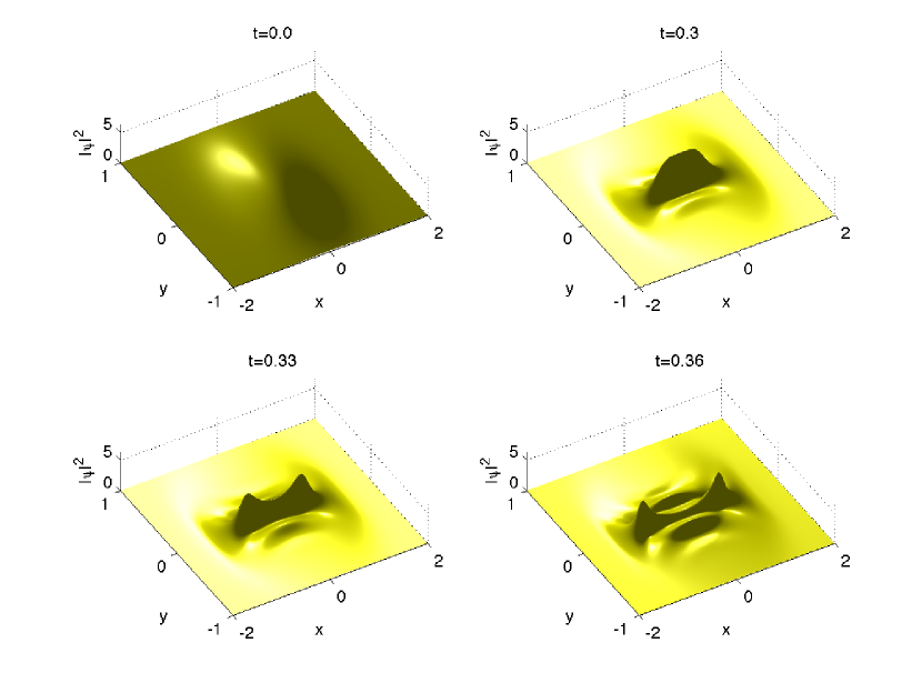
Figure 1. Solution to the hyperbolic NLS equation, equation (1) for $\beta=0$, for the initial data $\psi_{0}=\exp(-x^{2}-y^{2})$ for $\epsilon=0.1$ at different times.

At larger times, a regular pattern of peaks forms, see Fig. 2.

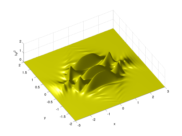
Figure 2. Solution to the hyperbolic NLS equation, equation (1) for $\beta=0$, for the initial data $\psi_{0}=\exp(-x^{2}-y^{2})$ for $\epsilon=0.1$ at $t=0.6$.

There is no indication of blow-up in this case as can be inferred from the $L_{\infty}$ norm of the solution in dependence of time in Fig. 3. The norm increases until a time of roughly $0.3$ and decreases then monotonically. The solution is well resolved in Fourier space as is obvious from the same figure where the Fourier coefficients are shown.

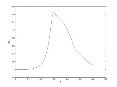
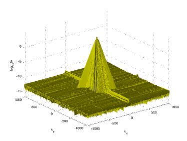
Figure 3. $L_{\infty}$-norm on the left and Fourier coefficients of the solution shown in Fig. 2 on the right.

4.2. Davey-Stewartson II solutions in the focusing case $\rho=-1$

For $\beta<1$ the behavior of solutions to the focusing DS II system is similar to the hyperbolic NLS case, but the solutions get more and more focused. This can be seen for instance in Fig. 4 where the solution for the same initial data as before is shown for $\beta=0.9$ for several values of $t$. This indicates already that one effect of the nonlocal term $\Phi$ is to increase the focusing effect for $\rho=-1$ in the spatial direction which is for the hyperbolic NLS defocusing. It is clear that the peaks are much more pronounced in this case, but the main focusing effect is still in the $y$-direction.

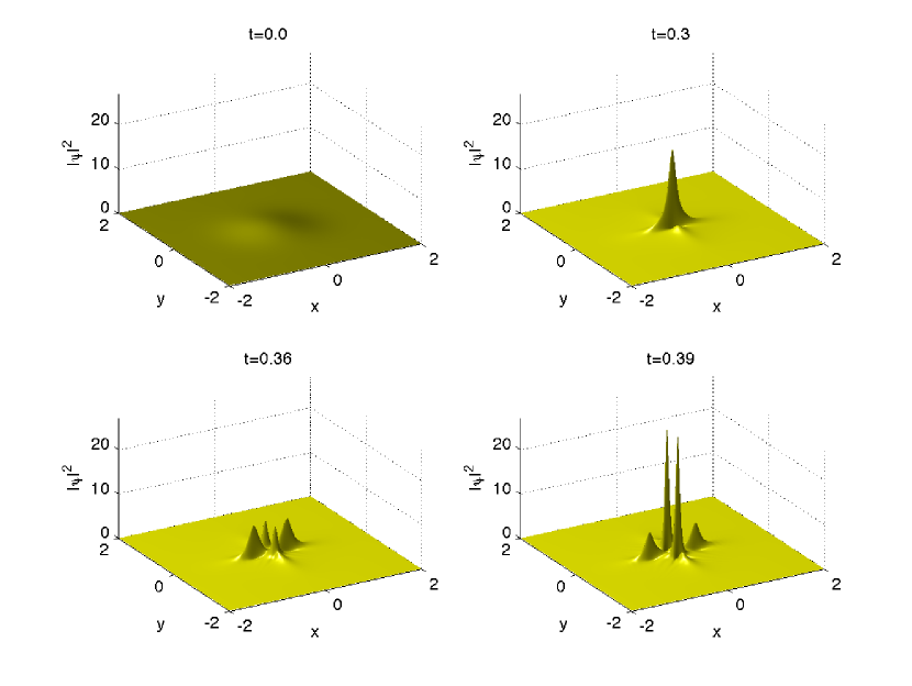
Figure 4. Solution to the DS II equation (1) for $\beta=0.9$, for the initial data $\psi_{0}=\exp(-x^{2}-y^{2})$ for $\epsilon=0.1$ at different times.

At time $t=0.6$, one finds again a regular pattern of peaks and no indication of blow-up, see Fig. 5.

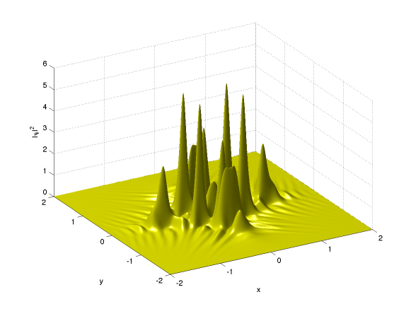
Figure 5. Solution to the DS II equation (1) for $\beta=0.9$, for the initial data $\psi_{0}=\exp(-x^{2}-y^{2})$ for $\epsilon=0.1$ at $t=0.6$.

The appearance of several peaks essentially rules out the possibility of blow-up since this would be expected for symmetric initial data at $x=y=0$. If the central peak splits into several smaller peaks, it is not clear how this could lead to a blow-up at a later time. The $L_{\infty}$ norm of the solution in dependence of time in Fig. 6 shows that there are several peaks appearing also here in contrast to the hyperbolic NLS case, but that it appears to decrease with time after the highest maximum. The solution is again well resolved in Fourier space as is visible in the same figure, but we had to use higher resolution and just reach machine precision in the $k_{y}$-direction.

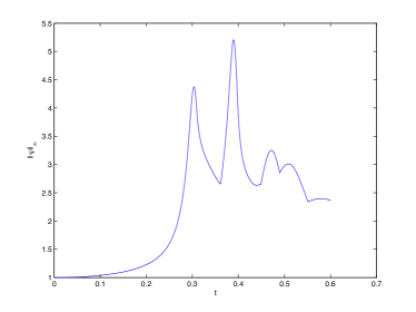
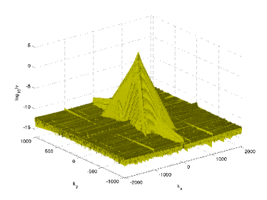
Figure 6. $L_{\infty}$-norm on the left and Fourier coefficients of the solution shown in Fig. 5 on the right.

It is remarkable that for the studied initial data, we obtain blow-up only for $\beta=1$ which will be discussed in detail in the next subsection. For $\beta>1$ we again observe a dispersive shock as for $\beta<1$. This can be seen for $\beta=1.1$ in Fig. 7 where no indication of blow-up can be seen.

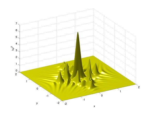
Figure 7. Solution to the DS II equation (1) for $\beta=1.1$, for the initial data $\psi_{0}=\exp(-x^{2}-y^{2})$ for $\epsilon=0.1$ at $t=0.6$.

The solution is also well resolved in Fourier space as is shown in Fig. 8.

Figure 8. Fourier coefficients of the solution shown in Fig. 7.

For larger values of $\beta$ the focusing effect in $x$-direction becomes even stronger. The resulting dispersive shock in Fig. 9 shows much more peaks than for smaller $\beta$, but there is again no indication of blow-up.

Figure 9. Solution to the DS II equation (1) for $\beta=2$, for the initial data $\psi_{0}=\exp(-x^{2}-y^{2})$ for $\epsilon=0.1$ at $t=0.6$.

In Fig. 10 we show that the situation of Fig. 9 is numerically well resolved.

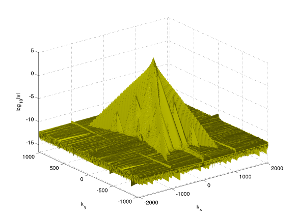
Figure 10. Fourier coefficients of the solution shown in Fig. 9.

One problem in the numerical study of the semiclassical limit and possible blow-up of the focusing DS II equation is the well known modulational instability of the focusing NLS equation. This implies in the present context that a lack of spatial resolution leads to a spurious growing in time of the Fourier coefficients for the high wave numbers as was for instance discussed in [30]. Thus it is important to resolve well the maximum of the solution even if one only wants to study the situation at a later time for which less resolution is required. Such a situation can be seen in Fig. 11. The largest peak is observed at $t\sim 0.15$. At this time the peak is not resolved in $k_{x}$-direction up to machine precision. This leads to some artifacts in the Fourier coefficients at later times for the high wave numbers. Note, however, that the coefficients still decrease to $10^{-10}$ and that the solution is thus well resolved.

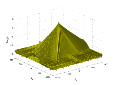
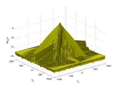
Figure 11. Fourier coefficients of the solution to the DS II equation (1) with $\beta=2$ for the initial data $\psi_{0}=\exp(-x^{2}-y^{2})$ for $\epsilon=0.1$ at $t=0.18$ on the left and at $t=0.6$ on the right for $N_{x}=N_{y}=2^{12}$.

4.3. Blow-up in focusing DS II solutions

As was shown in [27], for initial data of the form $\psi_{0}=\exp(-(x^{2}+\gamma y^{2}))$ with $\gamma>0$, a dispersive shock is observed as in the previous subsection if $\gamma\neq 1$. The situation is completely different in the integrable case $\beta=1$ for initial data $\psi_{0}=\exp(-x^{2}-y^{2})$ symmetric with respect to $x$ and $y$. In this case both the initial data and the equation are symmetric (up to complex conjugation) with respect to and exchange of the spatial coordinates. We use $N_{x}=N_{y}=2^{12}$ Fourier modes and $N_{t}=10^{4}$ time steps for $t<0.3$. The initial hump is focused in both directions $x$ and $y$ in a symmetric manner. It turns out that the initial maximum grows without bounds. The code is stopped at $t=0.2927$ since the fitting of the Fourier coefficients to the asymptotic formula (26) indicates that a singularity is closer to the real axis than the minimal resolved spatial distance (27) (the fitting is done just in $x$-direction because of the symmetry with respect to $x\to y$). Note that the factor $\mu$ in (26), which is in [27] slightly smaller than 1, is here still larger than 1 which would indicate a cusp with finite values of the $L_{\infty}$ norm. This simply indicates that we do not have enough resolution for the blow-up. To obtain better approximations for the value of $\mu$, obviously higher resolution on parallel computers would be needed as in [27], but we can make reliable statements on the type of blow-up below with the serial computing used in the present paper. The $L_{\infty}$ norm of the solution and the $L_{2}$ norm of the $x$-derivative can be seen in Fig. 12. Both seem to indicate a blow-up.

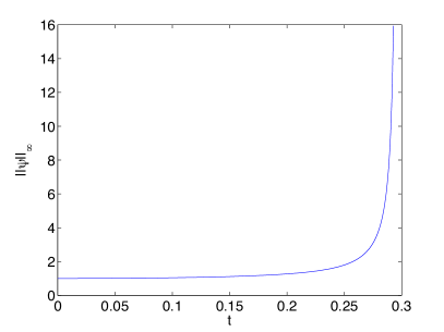
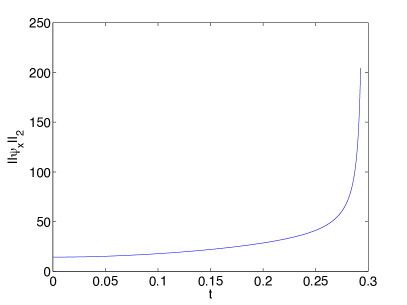
Figure 12. $L_{\infty}$-norm of the solution to the DS II equation (1) for $\beta=1$, for the initial data $\psi_{0}=\exp(-x^{2}-y^{2})$ for $\epsilon=0.1$ in dependence of $t$ on the left, and the corresponding $L_{2}$ norm of the $\psi_{x}$ on the right.

The appearance of blow-up is a very subtle and surprising phenomenon in DS II type systems since one does not expect blow-up in the cubic hyperbolic NLS equation. In order to obtain the actual blow-up time, we use the optimization algorithm [31], which is accessible via Matlab as the command fminsearch. For $t\approx t^{*}$, we fit for the $L_{\infty}$ of the solution and the $L_{2}$ norm of $x$-derivative to the expected asymptotic behavior (24). The $L_{\infty}$ norm thereby catches the local behavior of the solution close to blow-up, whereas the $L_{2}$ norm takes into account the solution on the whole computational domain. Thus the consistency of the fitting results provides a test of the quality of the numerics. The results of the fitting can be seen in Fig. 13. Fitting $\|\psi_{x}\|_{2}^{2}$ (normalized to 1 at $t=0$) for the last 500 computed time steps to $\kappa_{1}\ln(t^{*}-t)+\kappa_{2}$, we find $t^{*}=0.2946$, $\kappa_{1}=-1.047$ and $\kappa_{2}=-1.249$. Similarly, we get for $\|\psi\|_{\infty}$ the values $t^{*}=.2954$, $\kappa_{1}=-.822$ and $\kappa_{2}=-2.078$. Note the agreement of the blow-up times which shows the consistency of the fitting results within numerical precision. The fitting for the $L_{2}$ norm of $\psi_{x}$ agrees very well with the theoretical expectation $-1$, whereas the value for the $L_{\infty}$ norm is not close to the expected $1/2$. This indicates that we did not get close enough to blow-up for lack of resolution to catch the asymptotic behavior also locally near the blow-up. Note that these values are unchanged within numerical precision if only the last 100 computed time steps are used for the fitting.

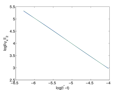
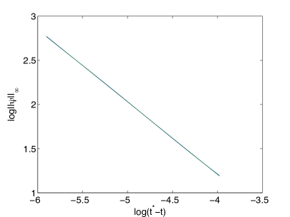
Figure 13. Fitting the logarithms of the $L_{2}$ norm of $\psi_{x}$ (left) and of the $L^{\infty}$ norm of $\psi$ (right) of the solution to the focusing DS II equation with $\beta=1$ with initial data $\psi_{0}=\exp(-x^{2}-y^{2})$ close to the blow-up. The fitted line $\kappa_{1}\ln(t^{*}-t)+\kappa_{2}$ (see the description) is given in green.

An interesting question is, whether the logarithmic corrections in (25) can also be seen within this approach, though certainly not in reliable way due to a lack of resolution. To test what can be seen with the present code, we do the same fitting as above for the last 20 computed time steps since the logarithmic corrections will be mainly noticeable for $t\approx t^{*}$, see e.g. the discussion in [25]. We denote the $L^{2}$ norm of the difference between the logarithm of the fitted norm and $\kappa_{1}\ln(t^{*}-t)+\kappa_{2}$ as the fitting error $\Delta_{2}$. We find $\Delta_{2}=0.0061$ for the $L^{2}$ norm of $\psi_{x}$. If we fit the same norms to $\tilde{\kappa}_{1}(\ln(t^{*}-t)-\ln\ln|\ln(t^{*}-t)|)+\tilde{\kappa}_{2}$, we get for the analogously defined fitting error $\tilde{\Delta}_{2}$ the value $0.0035$. Thus there appears to be an indication of logarithmic corrections, but this will have to be checked with higher resolution or an adaptive code.

4.4. Davey-Stewartson solutions in the defocusing case

In this subsection we will study the same initial data as above for the defocusing case, $\rho=1$. For the hyperbolic NLS this implies as already discussed an interchange of $x$ and $y$, i.e., of the focusing and of the defocusing direction. If the code is run for longer times, the pattern spreads more and more and the $L_{\infty}$ norm decreases. The solution at time $t=10$ can be seen in Fig. 14. The computation is carried out for $(x,y)\in[-10\pi,10\pi]\times[-10\pi,10\pi]$. Since the initial hump reaches the boundaries of the computational domain at large times, there are minor effects due to the imposed periodicity conditions which are visible in the Fourier coefficients in the same figure. It can be recognized, however, that the situation is still numerically well resolved.

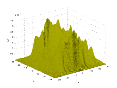
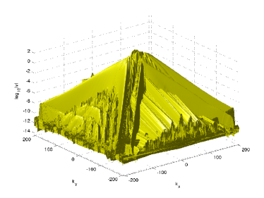
Figure 14. Solution to the hyperbolic NLS equations, i.e., equation (1) for $\beta=0$ and $\rho=1$ for the initial data $\psi_{0}=\exp(-x^{2}-y^{2})$ at $t=10$ and the corresponding Fourier coefficients.

These effects due to the boundary of the computational domain are also visible in the $L_{\infty}$ norm in Fig. 15 in the form of small oscillations. In the logarithmic plot we show also a line with slope $-1$ going through the endpoint of the graph of $\log||\psi||_{\infty}$. This suggests that the $L_{\infty}$ norm decreases as $1/t$. Since there appear to be no stable solutions to DS II (see the conjecture in [35] that initial data either lead to a blow-up or are radiated away), a $1/t$ decrease of the $L_{\infty}$ norm could be observed numerically for all cases without blow-up in the limit $t\to\infty$. In the focusing case, this is numerically difficult to address which is why we concentrate in this context on the defocusing case.

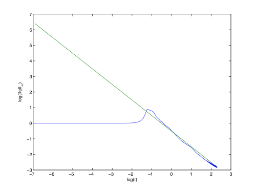
Figure 15. $L_{\infty}$-norm of the solution to the defocusing DS II equation (1) for $\beta=0$, for the initial data $\psi_{0}=\exp(-x^{2}-y^{2})$ for $\epsilon=0.1$ in dependence of $t$; the green line has slope $-1$ corresponding to a decrease of the $L_{\infty}$ norm proportional to $1/t$.

For larger values of $\beta$, the behavior of solutions to the defocusing DS II equations becomes more similar to what was shown for the integrable case in [28]. For $\beta=0.9$, this can be seen for instance in Fig. 16. The initial pulse is defocused to an almost pyramidal shape with a steeping of the gradient at the fronts. There are small oscillations in the vicinity of the region with strongest gradients.

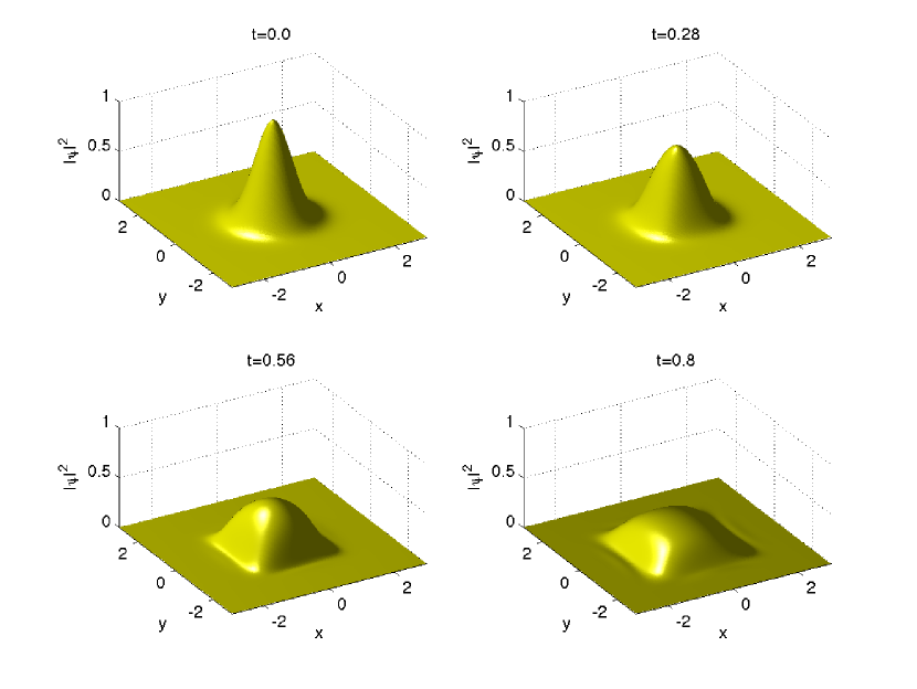
Figure 16. Solution to the defocusing DS II equation (1) for $\beta=0.9$, for the initial data $\psi_{0}=\exp(-x^{2}-y^{2})$ for $\epsilon=0.1$ at different times.

The $L_{\infty}$ norm appears again to decrease as $1/t$ for long times as can be seen in Fig. 17. The situation is very similar to the integrable case $\beta=1$ in the same figure.

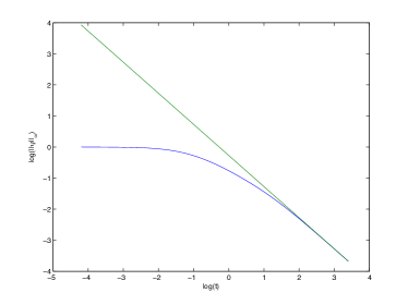
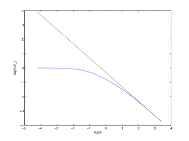
Figure 17. $L_{\infty}$-norm of the solution to the defocusing DS II equation (1) for $\beta=0.9$ on the left and $\beta=1$ on the right, for the initial data $\psi_{0}=\exp(-x^{2}-y^{2})$ for $\epsilon=0.1$ in dependence of $t$; the green lines have slope $-1$.

For larger values of $\beta$, the defocusing effect is more pronounced in $x$-direction as can be seen in Fig. 18. The long time behavior is, however, as before, the $L_{\infty}$ norm appears to decrease as $1/t$.

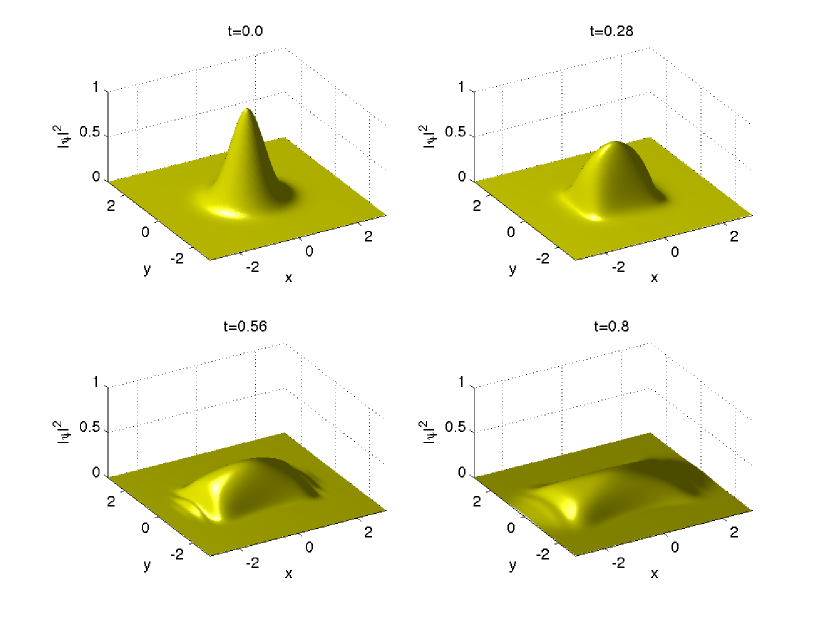
Figure 18. Solution to the defocusing DS II equation (1) for $\beta=2$, for the initial data $\psi_{0}=\exp(-x^{2}-y^{2})$ for $\epsilon=0.1$ at different times.

5. Conclusion

The numerical simulations above together with the results obtained by Inverse Scattering techniques suggest the following conjectures:

1. Cubic hyperbolic NLS: We expect global solutions, with dispersion of the sup norm as $O(1/t).$

2. Defocusing DS II type systems: We expect the same behavior as for the hyperbolic cubic NLS.

3. Focusing DS II type systems. We do not expect finite time blow-up except in the integrable case $\beta=1$ for initial data invariant under an exchange of the $x$ and $y$. In particular no localized solitary waves should exist when $\beta\neq 1.$

4. Blow-up for the focusing integrable system may occur for initial data different to the ones given by Ozawa’s construction, say a Gaussian with sufficiently high mass and invariant under the transformation $x\to y$. Proving such a surprising result should not be easy since the integrable focusing DS system belongs to the "non hyperbolic cubic NLS family" (the dynamic of which is likely to be governed by dispersion) and the standard methods of blow-up for say, the focusing cubic NLS equation (explicit blow-up via a ground state solution and a pseudo-conformal law or virial techniques) clearly do not apply here. Moreover this blow-up, if confirmed, appears to be highly non structurally stable since our simulations suggest that it does not persist in the non integrable case. In particular, finding a criterion of blow-up such as the one obtained in the $L^{2}$ critical cubic NLS is an interesting open question.

References

- [1] M.J. Ablowitz and P.A. Clarkson, Solitons, nonlinear evolution equations and inverse scattering, London Mathematical Society Lecture Notes series 149, Cambridge University Press, (1991).
- [2] M.J. Ablowitz and H. Segur, On the evolution of packets of water waves, J. Fluid Mech. 92 (1979), 691-715.
- [3] V.A. Arkadiev, A.K. Pogrebkov and M.C. Polivanov, Inverse scattering transform and soliton solution for Davey-Stewartson II equation, Physica D 36 (1089), 188-197.
- [4] D.J. Benney and G.J. Roskes, Waves instabilities, Stud. Appl. Math. 48 (1969), 377-385.
- [5] C. Besse and C.H. Bruneau, Numerical study of elliptic-hyperbolic Davey-Stewartson system: dromions simulation and blow-up, Math. Mod. and Meth. in Appl. Sciences 8, (8) (1998), 1363-1386.
- [6] C. Besse, N. Mauser and H.-P. Stimming, Numerical study of the Davey-Stewartson system, M2AN Math. Model. Numer. Anal., 38, (6) (2004), 1035-1054.
- [7] T. Cazenave, and F.B. Weissler, Some remarks on the nonlinear Schrödinger equation in the critical case, in Nonlinear semigroups, partial differential equations and attractors (Washington, DC, 1987), 18-29, Lecture Notes in Math., 1394, Springer, Berlin, 1989.
- [8] R. Cipolatti, On the existence of standing waves for a Davey-Stewartson system, Comm. Partial Differential Equations 17 (1992), no. 5-6, 967-988.
- [9] R. Cipolatti, On the instability of ground states for a Davey-Stewartson system, Ann.Inst. H. Poincaré, Phys.Théor. 58 (1993), 85-104.
- [10] T. Colin, Rigorous derivation of the nonlinear Schrödinger equation and Davey-Stewartson systems from quadratic hyperbolic systems, Asymptotic Analysis 31 (2002), 69-91.
- [11] T. Colin and D. Lannes, Justification of and long-wave correction to Davey-Stewartson systems from quadratic hyperbolic systems, Disc. Cont. Dyn. Systems 11 (1) (2004), 83-100.
- [12] A. Davey and K. Stewartson, One three-dimensional packets of water waves, Proc. Roy. Soc. Lond. A 338 (1974), 101-110.
- [13] V.D. Djordjevic and L.G. Redekopp, On two-dimensional packets of capillary-gravity waves, J. Fluid Mech. 79 (1977), 703-714.
- [14] T. Driscoll, A composite Runge-Kutta Method for the spectral Solution of semilinear PDEs, Journal of Computational Physics, 182 (2002), 357-367.
- [15] A. Fokas, D. Pelinovsky and C. Sulem, Interaction of lumps with a line soliton for the Davey-Stewartson II equation, Physica D, 152-153 (2001), 189-198.
- [16] J.-M. Ghidaglia and J.-C. Saut, On the initial value problem for the Davey-Stewartson systems, Nonlinearity, 3, (1990), 475-506.
- [17] J.-M. Ghidaglia and J.-C. Saut, Non existence of traveling wave solutions to nonelliptic nonlnear Schrödinger equations, J. Nonlinear Sci., 6 1996, 139-145.
- [18] J.-M. Ghidaglia and J.-C. Saut, On the Zakharov-Schulman equations, in Non- linear Dispersive Waves, L. Debnath Ed., World Scientific, 1992, 83-97.
- [19] J.-M. Ghidaglia and J.-C. Saut, Nonelliptic Schrödinger evolution equations, J. Nonlinear Science 3, (1993), 169-195.
- [20] N. Hayashi, Local existence in time of solutions to the elliptic-hyperbolic Davey-Stewartson system without smallness condition on the data, J. Analyse Mathématique 73, (1997), 133-164.
- [21] N. Hayashi and H. Hirota, Local existence in time of small solutions to the elliptic-hyperbolic Davey-Stewartson system in the usual Sobolev space, Proc. Edinburgh Math. Soc. 40 (1997), 563-581.
- [22] N. Hayashi and H. Hirota, Global existence and asymptotic behavior in time of small solutions to the elliptic-hyperbolic Davey-Stewartson system, Nonlinearity 9 (1996), 1387-1409.
- [23] O.M. Kiselev, Asymptotics of solutions of higher -dimensional integrable equations and their perturbations, J. of Mathematical Sciences, 138 (6) (2006), 6067-6230.
- [24] C. Klein and R. Peter, Numerical study of blow-up in solutions to generalized Korteweg-de Vries equations. Preprint available at arXiv:1307.0603
- [25] C. Klein, C. Sparber and P. Markowich, Numerical study of fractional Nonlinear Schrödinger equations, Preprint available at arXiv:1404.6262
- [26] C. Klein and K. Roidot, Numerical study of shock formation in the dispersionless Kadomtsev-Petviashvili equation and dispersive regularizations. Phys. D 265 (2013), 1–25.
- [27] C. Klein and K. Roidot, Numerical Study of the semiclassical limit of the Davey-Stewartson II equations. Prepint available at arXiv:1401.4745.
- [28] C. Klein and K. Roidot, Fourth order time-stepping for Kadomtsev-Petviashvili and Davey-Stewartson equations, SIAM Journal on Scientific Computing Vol. 33, No. 6, DOI: 10.1137/100816663 (2011).
- [29] C. Klein, B. Muite and K. Roidot, Numerical Study of Blowup in the Davey-Stewartson System, Discr. Cont. Dyn. Syst. B, Vol. 18, No. 5, 1361–1387 (2013).
- [30] C. Klein, Fourth order time-stepping for low dispersion Korteweg-de Vries and nonlinear Schrödinger equation, ETNA Vol. 29 116-135 (2008).
- [31] J. C. Lagarias, J. A. Reeds, M. H. Wright, and P. E. Wright, Convergence properties of the Nelder-Mead simplex method in low dimensions. SIAM J. Optimization 9 (1998), 112–147.
- [32] D. Lannes, Water waves: mathematical theory and asymptotics, Mathematical Surveys and Monographs, vol 188 (2013), AMS, Providence.
- [33] H. Leblond, Electromagnetic waves in ferromagnets, J. Phys. A 32 (45) (1999), 7907-7932.
- [34] F. Linares and G. Ponce, On the Davey-Stewartson systems, Ann. Inst. H. Poincaré Anal. Non Linéaire, 10 (1993), 523-548.
- [35] M. McConnell, A. Fokas, and B. Pelloni, Localised coherent Solutions of the DSI and DSII Equations a numerical Study, Mathematics and Computers in Simulation, 69 (2005), 424-438.
- [36] N. Mauser and K. Roidot, Numerical study of the transverse stability of NLS soliton solutions in several classes of NLS type equations, arXiv:1401.5349v1 [math-ph] 21 Jan 2014.
- [37] F. Merle and P. Raphaël, The blow-up dynamic and upper bound rate for critical nonlinear Schrödinger equation, Ann. of Math (2) 161 (1) (2005), 157-222.
- [38] S.L. Musher, A.M. Rubenchik and V.E. Zakharov, Hamiltonian approach to the description of nonlinear plasma phenomena, Phys. Rep. 129 (5) (1985), 285-366.
- [39] A. Newell and J.V. Moloney, Nonlinear Optics, Addison-Wesley (1992).
- [40] C. Obrecht and K. Roidot, In preparation.
- [41] M.Ohta, Stability and instability of standing waves for the generalized Davey-Stewartson system, Diff. Int. Eq. 8 (1995), 1775-1788.
- [42] M.Ohta, Instability of standing waves for the generalized Davey-Stewartson system, Ann. Inst. H. Poincaré, Phys. Théor. 62 (1995), 69-80.
- [43] M.Ohta, Blow-up solutions and strong instability of standing waves for the generalized Davey-Stewartson system, Ann. Inst. H. Poincaré, Phys. Théor. 63 (1995), 111-117.
- [44] T. Ozawa, Exact blow-up solutions to the Cauchy problem for the Davey-Stewartson systems, Proc.Roy. Soc. London A, 436 (1992), 345-349.
- [45] G. Papanicolaou, C. Sulem, P.-L. Sulem and X.P. Wang, The focusing singularity of the Davey-Stewartson equations for gravity-capillary waves, Physica D 72 (1994), 61-86.
- [46] D. Pelinovsky and C. Sulem, Embedded solitons of the Davey-Stewartson II equation, CRM Proceedings and Lecture Notes, Volume 27 (2001), ed. C. Sulem and I.M. Sigal (2001), 135-145.
- [47] D.E. Pelinovsky, E.A. Rouvinskaya, O.E. Kurkina and B. Deconincks, Short-wave transverse instability of line solitons of the two-dimensional hyperbolic nonlinear Schrödinger equation, Theoretical and Mathematical Physics, 179 (1) (2014), 452�461.
- [48] P. A. Perry, Global well-posedness and long time asymptotics for the defocussing Davey-Stewartson II equation in , arXiv:1110.5589v2, 26 Sep 2012.
- [49] F. Rousset and N. Tzvetkov, Transverse nonlinear instability for some Hamiltonian PDE’s, J. Math.Pures Appl. 90 (2008), 550-590.
- [50] F. Rousset and N. Tzvetkov, Transverse nonlinear instability for two-dimensional dispersive models, Ann. IHP, Analyse Non Linéaire, 26 (2009), 477-496.
- [51] F. Rousset and N. Tzvetkov, A simple criterion of transverse linear instability for solitary waves, Math. Res. Lett., 17 (2010), 157-169
- [52] E.I. Schulman, On the integrability of equations of Davey-Stewartson type, Theor.Math. Phys. 56 (1983), 131-136.
- [53] C. Sulem, P. Sulem, and H. Frisch, Tracing complex singularities with spectral methods, J. Comp. Phys., 50 (1983), pp. 138–161.
- [54] C. Sulem and P.L. Sulem, The nonlinear Schrödinger equation: Self-Focusing and Wave Collapse. Springer Series in Mathematical Sciences Vol. 139, Springer Verlag 1999.
- [55] L.Y. Sung, An inverse scattering transform for the Davey-Stewartson equations. I, J. Math. Anal. Appl. 183 (1) (1994), 121-154.
- [56] L.Y. Sung, An inverse scattering transform for the Davey-Stewartson equations. II, J. Math. Anal. Appl. 183 (2) (1994), 289-325.
- [57] L.Y. Sung, An inverse scattering transform for the Davey-Stewartson equations. III, J. Math. Anal. Appl. 183 (3) (1994), 477-494.
- [58] L.-Y. Sung, Long-Time Decay of the Solutions of the Davey-Stewartson II Equations, J. Non- linear Sci., 5 (1995), pp. 433-452.
- [59] V.E. Zakharov, Stability of periodic waves of finite amplitude on the surface of a deep fluid, J. Appl. Mech. Tech. Phys. 2 (1968) 190-194.
- [60] V. E. Zakharov and A. M. Rubenchik, Nonlinear interaction of high-frequency and low frequency waves, Prikl. Mat. Techn. Phys., (1972), 84-98.
- [61] V. E. Zakharov and, E. I. Schulman, Degenerate dispersion laws, motion invariants and kinetic equations, Physica 1D (1980), 192-202.
- [62] V. E. Zakharov and, E. I. Schulman, Integrability of nonlinear systems and perturbation theory, in What is integrability? (V.E. Zakharov, ed.), (1991), 185-250, Springer Series on Nonlinear Dynamics, Springer-Verlag.