A variational approach to stable principal component pursuit

Abstract

We introduce a new convex formulation for stable principal component pursuit (SPCP) to decompose noisy signals into low-rank and sparse representations. For numerical solutions of our SPCP formulation, we first develop a convex variational framework and then accelerate it with quasi-Newton methods. We show, via synthetic and real data experiments, that our approach offers advantages over the classical SPCP formulations in scalability and practical parameter selection.

1 INTRODUCTION

Linear superposition is a useful model for many applications, including nonlinear mixing problems. Surprisingly, we can perfectly distinguish multiple elements in a given signal using convex optimization as long as they are concise and look sufficiently different from one another. Popular examples include robust principal component analysis (RPCA) where we decompose a signal into low rank and sparse components and stable principal component pursuit (SPCP), where we also seek an explicit noise component within the RPCA decomposition. Applications include alignment of occluded images (Peng et al., 2012), scene triangulation (Zhang et al., 2011), model selection (Chandrasekaran et al., 2012), face recognition, and document indexing (Candès et al., 2011).

The SPCP formulation can be mathematically stated as follows. Given a noisy matrix $Y\in\mathbb{R}^{m\times n}$, we decompose it as a sum of a low-rank matrix $L$ and a sparse matrix $S$ via the following convex program

$$\operatorname*{minimize}_{L,S}\;{\left|\kern-1.07639pt\left|\kern-1.07639pt\left|L\right|\kern-1.07639pt\right|\kern-1.07639pt\right|}_{*}+\lambda_{\text{sum}}\|S\|_{1} \text{SPCP}_{\text{sum}}$$ ()

$$\text{subject to}\;\|L+S-Y\|_{F}\leq\varepsilon,$$

where the 1-norm $\|\cdot\|_{1}$ and nuclear norm ${\left|\kern-1.07639pt\left|\kern-1.07639pt\left|\cdot\right|\kern-1.07639pt\right|\kern-1.07639pt\right|}_{*}$ are given by $\|S\|_{1}=\sum_{i,j}|s_{i,j}|,{\left|\kern-1.07639pt\left|\kern-1.07639pt\left|L\right|\kern-1.07639pt\right|\kern-1.07639pt\right|}_{*}=\sum_{i}\sigma_{i}(L),$ where $\sigma(L)$ is the vector of singular values of $L$. In ($\text{SPCP}_{\text{sum}}$), the parameter $\lambda_{\text{sum}}>0$ controls the relative importance of the low-rank term $L$ vs. the sparse term $S$, and the parameter $\varepsilon$ accounts for the unknown perturbations $Y-(L+S)$ in the data not explained by $L$ and $S$.

When $\varepsilon=0$, ($\text{SPCP}_{\text{sum}}$) is the “robust PCA” problem as analyzed by Chandrasekaran et al. (2009); Candès et al. (2011), and it has perfect recovery guarantees under stylized incoherence assumptions. There is even theoretical guidance for selecting a minimax optimal regularization parameter $\lambda_{\text{sum}}$ (Candès et al., 2011). Unfortunately, many practical problems only approximately satisfy the idealized assumptions, and hence, we typically tune RPCA via cross-validation techniques. SPCP further complicates the practical tuning due to the additional parameter $\varepsilon$.

To cope with practical tuning issues of SPCP, we propose the following new variant called “max-SPCP”:

$$\operatorname*{minimize}_{L,S}\;\max\left({\left|\kern-1.07639pt\left|\kern-1.07639pt\left|L\right|\kern-1.07639pt\right|\kern-1.07639pt\right|}_{*},\lambda_{\text{max}}\|S\|_{1}\right) \text{SPCP}_{\text{max}}$$ ()

$$\text{subject to}\;\|L+S-Y\|_{F}\leq\varepsilon,$$

where $\lambda_{\text{max}}>0$ acts similar to $\lambda_{\text{sum}}$. Our work shows that this new formulation offers both modeling and computational advantages over ($\text{SPCP}_{\text{sum}}$).

Cross-validation with ($\text{SPCP}_{\text{max}}$) to estimate $(\lambda_{\text{max}},\varepsilon)$ is significantly easier than estimating $(\lambda_{\text{sum}},\varepsilon)$ in ($\text{SPCP}_{\text{sum}}$). For example, given an oracle that provides an ideal separation $Y\simeq L_{\text{oracle}}+S_{\text{oracle}}$, we can use $\varepsilon=\|L_{\text{oracle}}+S_{\text{oracle}}-Y\|_{F}$ in both cases. However, while we can estimate $\lambda_{\text{max}}=\|L_{\text{oracle}}\|_{*}/\|S_{\text{oracle}}\|_{1}$, it is not clear how to choose $\lambda_{\text{sum}}$ from data. Such cross validation can be performed on a similar dataset, or it could be obtained from a probabilistic model.

Our convex approach for solving ($\text{SPCP}_{\text{sum}}$) generalizes to other source separation problems (Baldassarre et al., 2013) beyond SPCP. Both ($\text{SPCP}_{\text{max}}$) and ($\text{SPCP}_{\text{sum}}$) are challenging to solve when the dimensions are large. We show in this paper that these problems can be solved more efficiently by solving a few (typically 5 to 10) subproblems of a different functional form. While the efficiency of the solution algorithms for ($\text{SPCP}_{\text{sum}}$) relies heavily on the efficiency of the 1-norm and nuclear norm projections, the efficiency of our solution algorithm ($\text{SPCP}_{\text{max}}$) is preserved for arbitrary norms. Moreover, ($\text{SPCP}_{\text{max}}$) allows a faster algorithm in the standard case, discussed in Section 6.

2 A PRIMER ON SPCP

The theoretical and algorithmic research on SPCP formulations (and source separation in general) is rapidly evolving. Hence, it is important to set the stage first in terms of the available formulations to highlight our contributions.

To this end, we illustrate ($\text{SPCP}_{\text{sum}}$) and ($\text{SPCP}_{\text{max}}$) via different convex formulations. Flipping the objective and the constraints in ($\text{SPCP}_{\text{max}}$) and ($\text{SPCP}_{\text{sum}}$), we obtain the following convex programs

$$\operatorname*{minimize}_{L,S}\;\frac{1}{2}\|L+S-Y\|_{F}^{2} \text{flip-SPCP}_{\text{sum}}$$ ()

$$\text{s.t.}\quad{\left|\kern-1.07639pt\left|\kern-1.07639pt\left|L\right|\kern-1.07639pt\right|\kern-1.07639pt\right|}_{*}+\lambda_{\text{sum}}\|S\|_{1}\leq\tau_{\text{sum}}$$

$$\operatorname*{minimize}_{L,S}\;\frac{1}{2}\|L+S-Y\|_{F}^{2} \text{flip-SPCP}_{\text{max}}$$ ()

$$\text{s.t.}\quad\max({\left|\kern-1.07639pt\left|\kern-1.07639pt\left|L\right|\kern-1.07639pt\right|\kern-1.07639pt\right|}_{*},\lambda_{\text{max}}\|S\|_{1})\leq\tau_{\text{max}}$$

Remark 2.1.

The solutions of ($\text{flip-SPCP}_{\text{sum}}$) and ($\text{flip-SPCP}_{\text{max}}$) are related to the solutions of ($\text{SPCP}_{\text{sum}}$) and ($\text{SPCP}_{\text{max}}$) via the Pareto frontier by Aravkin et al. (2013a, Theorem 2.1). If the constraint $\|L+S-Y\|\leq\varepsilon$ is tight at the solution, then there exist corresponding parameters $\tau_{\text{sum}}(\varepsilon)$ and $\tau_{\text{max}}(\varepsilon)$, for which the optimal value of ($\text{flip-SPCP}_{\text{sum}}$) and ($\text{flip-SPCP}_{\text{max}}$) is $\varepsilon$, and the corresponding optimal solutions $(\overline{S}_{s},\overline{L}_{s})$ and $(\overline{S}_{m},\overline{L}_{m})$ are also optimal for ($\text{SPCP}_{\text{sum}}$) and ($\text{SPCP}_{\text{max}}$).

For completeness, we also include the Lagrangian formulation, which is covered by our new algorithm:

$$\operatorname*{minimize}_{L,S}\;\lambda_{\text{L}}{\left|\kern-1.07639pt\left|\kern-1.07639pt\left|L\right|\kern-1.07639pt\right|\kern-1.07639pt\right|}_{*}+\lambda_{\text{S}}\|S\|_{1}+\frac{1}{2}\|L+S-Y\|_{F}^{2}$$ (Lag-SPCP)

Problems ($\text{flip-SPCP}_{\text{max}}$) and ($\text{flip-SPCP}_{\text{sum}}$) can be solved using projected gradient and accelerated gradient methods. The disadvantage of some of these formulations is that it may not be clear how to tune the parameters. Surprisingly, an algorithm we propose in this paper can solve ($\text{SPCP}_{\text{max}}$) and ($\text{SPCP}_{\text{sum}}$) using a sequence of flipped problems that specifically exploits the structured relationship cited in Remark 2.1. In practice, we will see that better tuning also leads to faster algorithms, e.g., fixing $\varepsilon$ ahead of time to an estimated ‘noise floor’ greatly reduces the amount of required computation if parameters are to be selected via cross-validation.

Finally, we note that in some cases, it is useful to change the $\|L+S-Y\|_{F}$ term to $\|\mathcal{A}(L+S-Y)\|_{F}$ where $\mathcal{A}$ is a linear operator. For example, let $\Omega$ be a subset of the indices of a $m\times n$ matrix. We may only observe $Y$ restricted to these entries, denoted $\mathcal{P}_{\Omega}(Y)$, in which case we choose $\mathcal{A}=\mathcal{P}_{\Omega}$. Most existing RPCA/SPCP algorithms adapt to the case $\mathcal{A}=\mathcal{P}_{\Omega}$ but this is due to the strong properties of the projection operator $\mathcal{P}_{\Omega}$. The advantage of our approach is that it seamlessly handles arbitrary linear operators $\mathcal{A}$. In fact, it also generalizes to smooth misfit penalties, that are more robust than the Frobenius norm, including the Huber loss. Our results also generalize to some other penalties on $S$ besides the 1-norm.

The paper proceeds as follows. In Section 3, we describe previous work and algorithms for SPCP and RPCA. In Section 4, we cast the relationships between pairs of problems ($\text{flip-SPCP}_{\text{sum}}$), ($\text{SPCP}_{\text{sum}}$) and ($\text{flip-SPCP}_{\text{max}}$), ($\text{SPCP}_{\text{max}}$) into a general variational framework, and highlight the product-space regularization structure that enables us solve the formulations of interest using corresponding flipped problems. We discuss computationally efficient projections as optimization workhorses in Section 5, and develop new accelerated projected quasi-Newton methods for the flipped and Lagrangian formulations in Section 6. Finally, we demonstrate the efficacy of the new solvers and the overall formulation on synthetic problems and a real cloud removal example in Section 7, and follow with conclusions in Section 8.

3 PRIOR ART

While problem ($\text{SPCP}_{\text{sum}}$) with $\varepsilon=0$ has several solvers (e.g., it can be solved by applying the widely known Alternating Directions Method of Multipliers (ADMM)/Douglas-Rachford method (Combettes & Pesquet, 2007)), the formulation assumes the data are noise free. Unfortunately, the presence of noise we consider in this paper introduces a third term in the ADMM framework, where the algorithm is shown to be non-convergent (Chen et al., 2013). Interestingly, there are only a handful of methods that can handle this case. Those using smoothing techniques no longer promote exactly sparse and/or exactly low-rank solutions (Aybat et al., 2013). Those using dual decomposition techniques require high iteration counts. Because each step requires a partial singular value decomposition (SVD) of a large matrix, it is critical that the methods only take a few iterations.

As a rough comparison, we start with related solvers that solve ($\text{SPCP}_{\text{sum}}$) for $\varepsilon=0$. Wright et al. (2009a) solves an instance of ($\text{SPCP}_{\text{sum}}$) with $\varepsilon=0$ and a $800\times 800$ system in $8$ hours. By switching to the (Lag-SPCP) formulation, Ganesh et al. (2009) uses the accelerated proximal gradient method (Beck & Teboulle, 2009) to solve a $1000\times 1000$ matrix in under one hour. This is improved further in Lin et al. (2010) which again solves ($\text{SPCP}_{\text{sum}}$) with $\varepsilon=0$ using the augmented Lagrangian and ADMM methods and solves a $1500\times 1500$ system in about a minute. As a prelude to our results, our method can solve some systems of this size in about $10$ seconds (c.f., Fig. 1).

In the case of ($\text{SPCP}_{\text{sum}}$) with $\varepsilon>0$, Tao & Yuan (2011) propose the alternating splitting augmented Lagrangian method (ASALM), which exploits separability of the objective in the splitting scheme, and can solve a $1500\times 1500$ system in about five minutes.

The partially smooth proximal gradient (PSPG) approach of Aybat et al. (2013) smooths just the nuclear norm term and then applies the well-known FISTA algorithm (Beck & Teboulle, 2009). Aybat et al. (2013) show that the proximity step can be solved efficiently in closed-form, and the dominant cost at every iteration is that of the partial SVD. They include some examples on video, lopsided matrices: $25000\times 300$ or so, in about 1 minute). solving $1500\times 1500$ formulations in under half a minute.

The nonsmooth adaptive Lagrangian (NSA) algorithm of Aybat & Iyengar (2014) is a variant of the ADMM for ($\text{SPCP}_{\text{sum}}$), and makes use of the insight of Aybat et al. (2013). The ADMM variant is interesting in that it splits the variable $L$, rather than the sum $L+S$ or residual $L+S-Y$. Their experiments solve a 1500 $\times$ 1500 synthetic problems in between 16 and 50 seconds (depending on accuracy) .

Shen et al. (2014) develop a method exploiting low-rank matrix factorization scheme, maintaining $L=UV^{T}$. This technique has also been effectively used in practice for matrix completion (Lee et al., 2010; Recht & Ré, 2011; Aravkin et al., 2013b), but lacks a full convergence theory in either context. The method of (Shen et al., 2014) was an order of magnitude faster than ASALM, but encountered difficulties in some experiments where the sparse component dominated the low rank component in some sense. Mansour & Vetro (2014) attack the $\text{SPCP}_{\text{sum}}$ formulation using a factorized approach, together with alternating solves between $(U,V)$ and $S$. Non-convex techniques also include hard thresholding approaches, e.g. the approach of Kyrillidis & Cevher (2014). While the factorization technique may potentially speed up some of the methods presented here, we leave this to future work, and only work with convex formulations.

4 VARIATIONAL FRAMEWORK

Both of the formulations of interest ($\text{SPCP}_{\text{sum}}$) and ($\text{SPCP}_{\text{max}}$) can be written as follows:

$$\min\phi(L,S)\quad\text{s.t.}\quad\rho\left(L+S-Y\right)\leq\varepsilon.$$ (4.1)

Classic formulations assume $\rho$ to be the Frobenius norm; however, this restriction is not necessary, and we consider $\rho$ to be smooth and convex. In particular, $\rho$ can be taken to be the robust Huber penalty (Huber, 2004). Even more importantly, this formulation allows pre-composition of a smooth convex penalty with an arbitrary linear operator $\mathcal{A}$, which extends the proposed approach to a much more general class of problems. Note that a simple operator is already embedded in both formulations of interest:

$$L+S=\begin{bmatrix}I&I\end{bmatrix}\begin{bmatrix}L\\ S\end{bmatrix}.$$ (4.2)

Projection onto a set of observed indices $\Omega$ is also a simple linear operator that can be included in $\rho$. Operators may include different transforms (e.g., Fourier) applied to either $L$ or $S$.

The main formulations of interest differ only in the functional $\phi(L,S)$. For ($\text{SPCP}_{\text{sum}}$), we have

$$\phi_{\text{sum}}(L,S)={\left|\kern-1.07639pt\left|\kern-1.07639pt\left|L\right|\kern-1.07639pt\right|\kern-1.07639pt\right|}_{*}+\lambda_{\text{sum}}\|S\|_{1},$$

while for ($\text{SPCP}_{\text{max}}$),

$$\phi_{\text{max}}(L,S)=\max({\left|\kern-1.07639pt\left|\kern-1.07639pt\left|L\right|\kern-1.07639pt\right|\kern-1.07639pt\right|}_{*},\lambda_{\text{max}}\|S\|_{1}).$$

The problem class (4.1) falls into the class of problems studied by van den Berg & Friedlander (2008, 2011) for $\rho(\cdot)=\|\cdot\|^{2}$ and by Aravkin et al. (2013a) for arbitrary convex $\rho$. Making use of this framework, we can define a value function

$$v(\tau)=\min_{L,S}\rho\left(\mathcal{A}(L,S)-Y\right)\quad\text{s.t. }\phi(L,S)\leq\tau,$$ (4.3)

and use Newton’s method to find a solution to $v(\tau)=\varepsilon$. The approach is agnostic to the linear operator $\mathcal{A}$ (it can be of the simple form (4.2); include restriction in the missing data case, etc.).

For both formulations of interest, $\phi$ is a norm defined on a product space $\mathbb{R}^{n\times m}\times\mathbb{R}^{n\times m}$, since we can write

$$\phi_{\text{sum}}(L,S) =\left\|\begin{matrix}{\left|\kern-1.07639pt\left|\kern-1.07639pt\left|L\right|\kern-1.07639pt\right|\kern-1.07639pt\right|}_{*}\\ \lambda_{\text{sum}}\|S\|_{1}\end{matrix}\right\|_{1},$$ (4.4)

$$\phi_{\text{max}}(L,S) =\left\|\begin{matrix}{\left|\kern-1.07639pt\left|\kern-1.07639pt\left|L\right|\kern-1.07639pt\right|\kern-1.07639pt\right|}_{*}\\ \lambda_{\text{max}}\|S\|_{1}\end{matrix}\right\|_{\infty}.$$ (4.5)

In particular, both $\phi_{\text{sum}}(L,S)$ and $\phi_{\text{max}}(L,S)$ are gauges. For a convex set $C$ containing the origin, the gauge $\gamma\left(x\mid C\right)$ is defined by

$$\gamma\left(x\mid C\right)=\inf_{\lambda}\{\lambda:x\in\lambda C\}.$$ (4.6)

For any norm $\|\cdot\|$, the set defining it as a gauge is simply the unit ball $\mathbb{B}_{\|\cdot\|}=\{x:\|x\|\leq 1\}$. We introduce gauges for two reasons. First, they are more general (a gauge is a norm only if $C$ is bounded with nonempty interior and symmetric about the origin). For example, gauges trivially allow inclusion of non-negativity constraints. Second, definition (4.6) and the explicit set $C$ simplify the exposition of the following results.

In order to implement Newton’s method for (4.3), the optimization problem to evaluate $v(\tau)$ must be solved (fully or approximately) to obtain $(\overline{L},\overline{S})$. Then the $\tau$ parameter for the next (4.3) problem is updated via

$$\tau^{k+1}=\tau^{k}-\frac{v(\tau)-\tau}{v^{\prime}(\tau)}.$$ (4.7)

Given $(\overline{L},\overline{S})$, $v^{\prime}(\tau)$ can be written in closed form using (Aravkin et al., 2013a, Theorem 5.2), which simplifies to

$$v^{\prime}(\tau)=-\phi^{\circ}(\mathcal{A}^{T}\nabla\rho(\mathcal{A}(\overline{L},\overline{S})-Y)),$$ (4.8)

with $\phi^{\circ}$ denoting the polar gauge to $\phi$. The polar gauge is precisely $\gamma\left(x\mid C^{\circ}\right)$, with

$$C^{\circ}=\{v:\left\langle v,x\right\rangle\leq 1\quad\forall x\in C\}.$$ (4.9)

In the simplest case, where $\mathcal{A}$ is given by (4.2), and $\rho$ is the least squares penalty, the formula (4.8) becomes

$$v^{\prime}(\tau)=-\phi^{\circ}\left(\begin{bmatrix}\overline{L}+\overline{S}-Y\\ \overline{L}+\overline{S}-Y\end{bmatrix}\right).$$

The main computational challenge in the approach outlined in (4.3)-(4.8) is to design a fast solver to evaluate $v(\tau)$. Section 6 does just this.

The key to RPCA is that the regularization functional $\phi$ is a gauge over the product space used to decompose $Y$ into summands $L$ and $S$. This makes it straightforward to compute polar results for both $\phi_{\text{sum}}$ and $\phi_{\text{max}}$.

Theorem 4.1 (Max-Sum Duality for Gauges on Product Spaces).

Let $\gamma_{1}$ and $\gamma_{2}$ be gauges on $\mathbb{R}^{n_{1}}$ and $\mathbb{R}^{n_{2}}$, and consider the function

$$g(x,y)=\max\{\gamma_{1}(x),\gamma_{2}(y)\}.$$

Then $g$ is a gauge, and its polar is given by

$$g^{\circ}(z_{1},z_{2})=\gamma_{1}^{\circ}(z_{1})+\gamma_{2}^{\circ}(z_{2}).$$

Proof.

Let $C_{1}$ and $C_{2}$ denote the canonical sets corresponding to gauges $\gamma_{1}$ and $\gamma_{2}$. It immediately follows that $g$ is a gauge for the set $C=C_{1}\times C_{2}$, since

$$\inf\{\lambda\geq 0|(x,y)\in\lambda C\} =\inf\{\lambda|x\in\lambda C_{1}\text{ and }y\in\lambda C_{2}\}$$

$$=\max\{\gamma_{1}(x),\gamma_{2}(y)\}.$$

By (Rockafellar, 1970, Corollary 15.1.2), the polar of the gauge of $C$ is the support function of $C$, which is given by

$$\sup_{x\in C_{1},y\in C_{2}}\left\langle(x,y),(z_{1},z_{2})\right\rangle =\sup_{x\in C_{1}}\left\langle x,z_{1}\right\rangle+\sup_{y\in C_{2}}\left\langle y,z_{2}\right\rangle$$

$$=\gamma_{1}^{\circ}(z_{1})+\gamma_{2}^{\circ}(z_{2}).$$

∎

This theorem allows us to easily compute the polars for $\phi_{\text{sum}}$ and $\phi_{\text{max}}$ in terms of the polars of ${\left|\kern-1.07639pt\left|\kern-1.07639pt\left|\cdot\right|\kern-1.07639pt\right|\kern-1.07639pt\right|}_{*}$ and $\|\cdot\|_{1}$, which are the dual norms, the spectral norm and infinity norm, respectively.

Corollary 4.2 (Explicit variational formulae for ($\text{SPCP}_{\text{sum}}$) and ($\text{SPCP}_{\text{max}}$)).

We have

$$\phi_{\text{sum}}^{\circ}(Z_{1},Z_{2}) =\max\left\{{\left|\kern-1.07639pt\left|\kern-1.07639pt\left|Z_{1}\right|\kern-1.07639pt\right|\kern-1.07639pt\right|}_{2},\frac{1}{\lambda_{\text{sum}}}\|Z_{2}\|_{\infty}\right\}$$ (4.10)

$$\phi_{\text{max}}^{\circ}(Z_{1},Z_{2}) ={\left|\kern-1.07639pt\left|\kern-1.07639pt\left|Z_{1}\right|\kern-1.07639pt\right|\kern-1.07639pt\right|}_{2}+\frac{1}{\lambda_{\text{max}}}\|Z_{2}\|_{\infty},$$

where ${\left|\kern-1.07639pt\left|\kern-1.07639pt\left|X\right|\kern-1.07639pt\right|\kern-1.07639pt\right|}_{2}$ denotes the spectral norm (largest eigenvalue of $X^{T}X$).

This result was also obtained by (van den Berg & Friedlander, 2011, Section 9), but is stated only for norms. Theorem 4.1 applies to gauges, and in particular now allows asymmetric gauges, so non-negativity constraints can be easily modeled.

We now have closed form solutions for $v^{\prime}(\tau)$ in (4.8) for both formulations of interest. The remaining challenge is to design a fast solver for (4.3) for formulations ($\text{SPCP}_{\text{sum}}$) and ($\text{SPCP}_{\text{max}}$). We focus on this challenge in the remaining sections of the paper. We also discuss the advantage of ($\text{SPCP}_{\text{max}}$) from this computational perspective.

5 PROJECTIONS

In this section, we consider the computational issues of projecting onto the set defined by $\phi(L,S)\leq\tau$. For $\phi_{\text{max}}(L,S)=\max({\left|\kern-1.07639pt\left|\kern-1.07639pt\left|L\right|\kern-1.07639pt\right|\kern-1.07639pt\right|}_{*},\lambda_{\text{max}}\|S\|_{1})$ this is straightforward since the set is just the product set of the nuclear norm and $\ell_{1}$ norm balls, and efficient projectors onto these are known. In particular, projecting an $m\times n$ matrix (without loss of generality let $m\leq n$) onto the nuclear norm ball takes $\mathcal{O}(m^{2}n)$ operations, and projecting it onto the $\ell_{1}$-ball can be done on $\mathcal{O}(mn)$ operations using fast median-finding algorithms (Brucker, 1984; Duchi et al., 2008).

For $\phi_{\text{sum}}(L,S)={\left|\kern-1.07639pt\left|\kern-1.07639pt\left|L\right|\kern-1.07639pt\right|\kern-1.07639pt\right|}_{*}+\lambda_{\text{sum}}\|S\|_{1}$, the projection is no longer straightforward. Nonetheless, the following lemma shows this projection can be efficiently implemented.

Proposition 5.1.

(van den Berg & Friedlander, 2011, Section 5.2) Projection onto the scaled $\ell_{1}$-ball, that is, $\{x\in\mathbb{R}^{d}\mid\sum_{i=1}^{d}\alpha_{i}|x_{i}|\leq 1\}$ for some $\alpha_{i}>0$, can be done in $\mathcal{O}(d\log(d))$ time.

The proof of the proposition follows by noting that the solution can be written in a form depending only on a single scalar parameter, and this scalar can be found by sorting $(|x_{i}|/\alpha_{i})$ followed by appropriate summations. We conjecture that fast median-finding ideas could reduce this to $\mathcal{O}(d)$ in theory, the same as the optimal complexity for the $\ell_{1}$-ball.

Armed with the above proposition, we state an important lemma below. For our purposes, we may think of $S$ as a vector in $\mathbb{R}^{mn}$ rather than a matrix in $\mathbb{R}^{m\times n}$.

Lemma 5.2.

(van den Berg & Friedlander, 2011, Section 9.2) Let $L=U\Sigma V^{T}$ and $\Sigma=\operatorname{diag}(\sigma)$, and let $(S_{i})_{i=1}^{mn}$ be any ordering of the elements of $S$. Then the projection of $(L,S)$ onto the $\phi_{\text{sum}}$ ball is $(U\operatorname{diag}(\hat{\sigma})V^{T},\hat{S})$, where $(\hat{\sigma},\hat{S})$ is the projection onto the scaled $\ell_{1}$-ball $\{(\sigma,S)\mid\,\sum_{j=1}^{\min(m,n)}|\sigma_{j}|+\sum_{i=1}^{mn}\lambda_{\text{sum}}|S_{i}|\leq 1\}$.

Sketch of proof.

We need to solve

$$\min_{\{(L^{\prime},S^{\prime})\mid\,\phi_{\text{sum}}(L^{\prime},S^{\prime})\leq 1\}}\,\frac{1}{2}{\left\lVert{L^{\prime}-L}\right\rVert}_{F}^{2}+\frac{1}{2}{\left\lVert{S^{\prime}-S}\right\rVert}_{F}^{2}.$$

Alternatively, solve

$$\min_{S^{\prime}}\,\min_{\{L^{\prime}\mid\,{\left|\kern-0.75346pt\left|\kern-0.75346pt\left|L^{\prime}\right|\kern-0.75346pt\right|\kern-0.75346pt\right|}_{*}\leq 1-\lambda_{\text{sum}}\|S^{\prime}\|_{1}\}}\,\frac{1}{2}{\left\lVert{L^{\prime}-L}\right\rVert}_{F}^{2}+\frac{1}{2}{\left\lVert{S^{\prime}-S}\right\rVert}_{F}^{2}.$$

The inner minimization is equivalent to projecting onto the nuclear norm ball, and this is well-known to be soft-thresholding of the singular values. Since it depends only on the singular values, recombining the two minimization terms gives exactly a joint projection onto a scaled $\ell_{1}$-ball. ∎

Remark 5.1.

All the references to the $\ell_{1}$-ball can be replaced by the intersection of the $\ell_{1}$-ball and the non-negative cone, and the projection is still efficient. As noted in Section 4, imposing non-negativity constraints is covered by the gauge results of Theorem 4.1 and Corollary 4.2. Therefore, both the variational and efficient computational framework can be applied to this interesting case.

6 SOLVING THE SUB-PROBLEM VIA PROJECTED QUASI-NEWTON METHODS

In order to accelerate the approach, we can use quasi-Newton (QN) methods since the objective has a simple structure. The main challenge here is that for the ${\left|\kern-1.07639pt\left|\kern-1.07639pt\left|L\right|\kern-1.07639pt\right|\kern-1.07639pt\right|}_{*}$ term, it is tricky to deal with a weighted quadratic term (whereas for $\|S\|_{1}$, we can obtain a low-rank Hessian and solve it efficiently via coordinate descent).

We wish to solve ($\text{flip-SPCP}_{\text{max}}$). Let $X=(L,S)$ be the full variable, so we can write the objective function as $f(X)=\frac{1}{2}\|\mathcal{A}(X)-Y\|_{F}^{2}$. To simplify the exposition, we take $\mathcal{A}=(I,I)$ to be the $mn\times 2mn$ matrix, but the presented approach applies to general linear operators (including terms like $\mathcal{P}_{\Omega}$). The matrix structure of $L$ and $S$ is not important here, so we can think of them as $mn\times 1$ vectors instead of $m\times n$ matrices.

The gradient is $\nabla f(X)=\mathcal{A}^{T}(\mathcal{A}(X)-Y)$. For convenience, we use $r(X)=\mathcal{A}(X)-Y$ and

$$\nabla f(X)=\begin{pmatrix}\nabla_{L}f(X)\\ \nabla_{S}f(X)\end{pmatrix}=\mathcal{A}^{T}\begin{pmatrix}r(X)\\ r(X)\end{pmatrix},\quad r_{k}\equiv r(X_{k}).$$

The Hessian is $\mathcal{A}^{T}\mathcal{A}=\begin{pmatrix}I&I\\ I&I\end{pmatrix}$. We cannot simultaneously project $(L,S)$ onto their constraints with this Hessian scaling (doing so would solve the original problem!), since the Hessian removes separability. Instead, we use $(L_{k},S_{k})$ to approximate the cross-terms.

The true function is a quadratic, so the following quadratic expansion around $X_{k}=(L_{k},S_{k})$ is exact:

$$f(L,S)=f(X_{k}) +\left\langle\begin{pmatrix}\nabla_{L}f(X_{k})\\ \nabla_{S}f(X_{k})\end{pmatrix},\,\begin{pmatrix}L-L_{k}\\ S-S_{k}\end{pmatrix}\right\rangle$$

$$+\left\langle\begin{pmatrix}L-L_{k}\\ S-S_{k}\end{pmatrix},\,\nabla^{2}f\begin{pmatrix}L-L_{k}\\ S-S_{k}\end{pmatrix}\right\rangle$$

$$=f(X_{k}) +\left\langle\begin{pmatrix}r_{k}\\ r_{k}\end{pmatrix},\,\begin{pmatrix}L-L_{k}\\ S-S_{k}\end{pmatrix}\right\rangle$$

$$+\left\langle\begin{pmatrix}L-L_{k}\\ S-S_{k}\end{pmatrix},\,\begin{pmatrix}1&1\\ 1&1\end{pmatrix}\begin{pmatrix}L-L_{k}\\ S-S_{k}\end{pmatrix}\right\rangle$$

$$=f(X_{k}) +\left\langle\begin{pmatrix}r_{k}\\ r_{k}\end{pmatrix},\,\begin{pmatrix}L-L_{k}\\ S-S_{k}\end{pmatrix}\right\rangle$$

$$+\left\langle\begin{pmatrix}\mathbf{L}-L_{k}\\ \mathbf{S}-S_{k}\end{pmatrix},\,\begin{pmatrix}L-L_{k}+\mathbf{S}-S_{k}\\ \mathbf{L}-L_{k}+S-S_{k}\end{pmatrix}\right\rangle$$

The coupling of the second order terms, shown in bold, prevents direct 1-step minimization of $f$, subject to the nuclear and 1-norm constraints. The FISTA (Beck & Teboulle, 2009) and spectral gradient methods (SPG) (Wright et al., 2009b) replace the Hessian $\begin{pmatrix}I&I\\ I&I\end{pmatrix}$ with the upper bound $2\begin{pmatrix}I&0\\ 0&I\end{pmatrix}$, which solves the coupling issue, but potentially lose too much second order information. After comparing FISTA and SPG, we use the SPG method for solving ($\text{flip-SPCP}_{\text{sum}}$). However, for ($\text{flip-SPCP}_{\text{max}}$) (and for (Lag-SPCP), which has no constraints but rather non-smooth terms, which can be treated like constraints using proximity operators), the constraints are uncoupled and we can take a “middle road” approach, replacing

$$\left\langle\begin{pmatrix}\mathbf{L}-L_{k}\\ \mathbf{S}-S_{k}\end{pmatrix},\,\begin{pmatrix}L-L_{k}+\mathbf{S}-S_{k}\\ \mathbf{L}-L_{k}+S-S_{k}\end{pmatrix}\right\rangle$$

with

$$\left\langle\begin{pmatrix}L-L_{k}\\ S-S_{k}\end{pmatrix},\,\begin{pmatrix}L-L_{k}+\mathbf{S_{k}-S_{k-1}}\\ \mathbf{L_{k+1}-L_{k}}+S-S_{k}\end{pmatrix}\right\rangle.$$

The first term is decoupled, allowing us to update $L_{k}$, and then this is plugged into the second term in a Gauss-Seidel fashion. In practice, we also scale this second-order term with a number slightly greater than $1$ but less than $2$ (e.g., $1.25$) which leads to more robust behavior. We expect this “quasi-Newton” trick to do well when $S_{k+1}-S_{k}$ is similar to $S_{k}-S_{k-1}$.

7 NUMERICAL RESULTS

The numerical experiments are done with the algorithms suggested in this paper as well as code from PSPG (Aybat et al., 2013), NSA (Aybat & Iyengar, 2014), and ASALM (Tao & Yuan, 2011). We modified the other software as needed for testing purposes. PSPG, NSA and ASALM all solve ($\text{SPCP}_{\text{sum}}$), but ASALM has another variant which solves (Lag-SPCP) so we test this as well. All three programs also use versions of PROPACK from Larsen (1998); Becker & Candès (2008) to compute partial SVDs. Since the cost of a single iteration may vary among the solvers, we measure error as a function of time, not iterations. When a reference solution $(L^{\star},S^{\star})$ is available, we measure the (relative) error of a trial solution $(L,S)$ as $\|L-L^{\star}\|_{F}/\|L^{\star}\|_{F}+\|S-S^{\star}\|_{F}/\|S^{\star}\|_{F}$. The benchmark is designed so the time required to calculate this error at each iteration does not factor into the reported times. Since picking stopping conditions is solver dependent, we show plots of error vs time, rather than list tables. All tests are done in Matlab and the dominant computational time was due to matrix multiplications for all algorithms; all code was run in the same quad-core $1.6$ GHz i7 computer.

For our implementations of the ($\text{flip-SPCP}_{\text{max}}$), ($\text{flip-SPCP}_{\text{sum}}$) and (Lag-SPCP), we use a randomized SVD (Halko et al., 2011). Since the number of singular values needed is not known in advance, the partial SVD may be called several times (the same is true for PSPG, NSA and ASALM). Our code limits the number of singular values on the first two iterations in order to speed up calculation without affecting convergence. Unfortunately, the delicate projection involved in ($\text{flip-SPCP}_{\text{sum}}$) makes incorporating a partial SVD to this setting more challenging, so we use Matlab’s dense SVD routine.

7.1 Synthetic test with exponential noise

We first provide a test with generated data. The observations $Y\in\mathbb{R}^{m\times n}$ with $m=400$ and $n=500$ were created by first sampling a rank $20$ matrix $Y_{0}$ with random singular vectors (i.e., from the Haar measure) and singular values drawn from a uniform distribution with mean $0.1$, and then adding exponential random noise (with mean equal to one tenth the median absolute value of the entries of $Y_{0}$). This exponential noise, which has a longer tail than Gaussian noise, is expected to be captured partly by the $S$ term and partly by the $\|L+S-Y\|_{F}$ term.

Given $Y$, the reference solution $(L^{\star},S^{\star})$ was generated by solving (Lag-SPCP) to very high accuracy; the values $\lambda_{\text{L}}=0.25$ and $\lambda_{\text{S}}=10^{-2}$ were picked by hand tuning $(\lambda_{\text{L}},\lambda_{\text{S}})$ to find a value such that both $L^{\star}$ and $S^{\star}$ are non-zero. The advantage to solving (Lag-SPCP) is that knowledge of $(L^{\star},S^{\star},\lambda_{\text{L}},\lambda_{\text{S}})$ allows us to generate the parameters for all the other variants, and hence we can test different problem formulations.

With these parameters, $L^{\star}$ was rank 17 with nuclear norm $6.754$, $S^{\star}$ had 54 non-zero entries (most of them positive) with $\ell_{1}$ norm $0.045$, the normalized residual was $\|L^{\star}+S^{\star}-Y\|_{F}/\|Y\|_{F}=0.385$, and $\varepsilon=1.1086$, $\lambda_{\text{sum}}=0.04$, $\lambda_{\text{max}}=150.0593$, $\tau_{\text{sum}}=6.7558$ and $\tau_{\text{max}}=6.7540$.

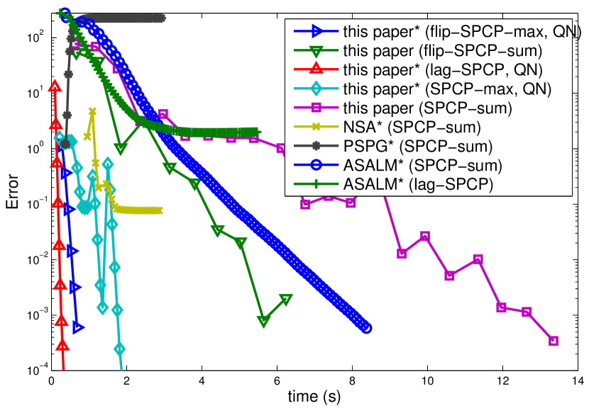
Figure 1: The exponential noise test. The asterisk in the legend means the method uses a fast SVD.

Results are shown in Fig. 1. Our methods for ($\text{flip-SPCP}_{\text{max}}$) and (Lag-SPCP) are extremely fast, because the simple nature of these formulations allows the quasi-Newton acceleration scheme of Section 6. In turn, since our method for solving ($\text{SPCP}_{\text{max}}$) uses the variational framework of Section 4 to solve a sequence of ($\text{flip-SPCP}_{\text{max}}$) problems, it is also competitive (shown in cyan in Figure 1). The jumps are due to re-starting the sub-problem solver with a new value of $\tau$, generated according to (4.7).

Our proximal gradient method for ($\text{flip-SPCP}_{\text{sum}}$), which makes use of the projection in Lemma 5.2, converges more slowly, since it is not easy to accelerate with the quasi-Newton scheme due to variable coupling, and it does not make use of fast SVDs. Our solver for ($\text{SPCP}_{\text{sum}}$), which depends on a sequence of problems ($\text{flip-SPCP}_{\text{sum}}$), converges slowly.

The ASALM performs reasonably well, which was unexpected since it was shown to be worse than NSA and PSPG in Aybat et al. (2013); Aybat & Iyengar (2014). The PSPG solver converges to the wrong answer, most likely due to a bad choice of the smoothing parameter $\mu$; we tried choosing several different values other than the default but did not see improvement for this test (for other tests, not shown, tweaking $\mu$ helped significantly). The NSA solver reaches moderate error quickly but stalls before finding a highly accurate solution.

7.2 Synthetic test from Aybat & Iyengar (2014)

We show some tests from the test setup of Aybat & Iyengar (2014) in the $m=n=1500$ case. The default setting of $\lambda_{\text{sum}}=1/\sqrt{\max(m,n)}$ was used, and then the NSA solver was run to high accuracy to obtain a reference solution $(L^{\star},S^{\star})$. From the knowledge of $(L^{\star},S^{\star},\lambda_{\text{sum}})$, one can generate $\lambda_{\text{max}},\tau_{\text{sum}},\tau_{\text{max}},\varepsilon$, but not $\lambda_{\text{S}}$ and $\lambda_{\text{L}}$, and hence we did not test the solvers for (Lag-SPCP) in this experiment. The data was generated as $Y=L_{0}+S_{0}+Z_{0}$, where $L_{0}$ was sampled by multiplication of $m\times r$ and $r\times n$ normal Gaussian matrices, $S_{0}$ had $p$ randomly chosen entries uniformly distributed within $[-100,100]$, and $Z_{0}$ was white noise chosen to give a SNR of $45$ dB. We show three tests that vary the rank from $\{0.05,0.1\}\cdot\min(m,n)$ and the sparsity ranging from $p=\{0.05,0.1\}\cdot mn$. Unlike Aybat & Iyengar (2014), who report error in terms of a true noiseless signal $(L_{0},S_{0})$, we report the optimization error relative to $(L^{\star},S^{\star})$.

For the first test (with $r=75$ and $p=0.05\times mn$), $L^{\star}$ had rank $786$ and nuclear norm $111363.9$; $S^{\star}$ had $75.49\%$ of its elements nonzero and $\ell_{1}$ norm $5720399.4$, and $\|L^{\star}+S^{\star}-Y^{\star}\|_{F}/\|Y\|_{F}=1.5\cdot 10^{-4}$. The other parameters were $\varepsilon=3.5068$, $\lambda_{\text{sum}}=0.0258$, $\lambda_{\text{max}}=0.0195$, $\tau_{\text{sum}}=2.5906\cdot 10^{5}$ and $\tau_{\text{max}}=1.1136\cdot 10^{5}$. An interesting feature of this test is that while $L_{0}$ is low-rank, $L^{\star}$ is nearly low-rank but with a small tail of significant singular values until number $786$. We expect methods to converge quickly to low-accuracy where only a low-rank approximation is needed, and then slow down as they try to find a larger rank highly-accurate solution.

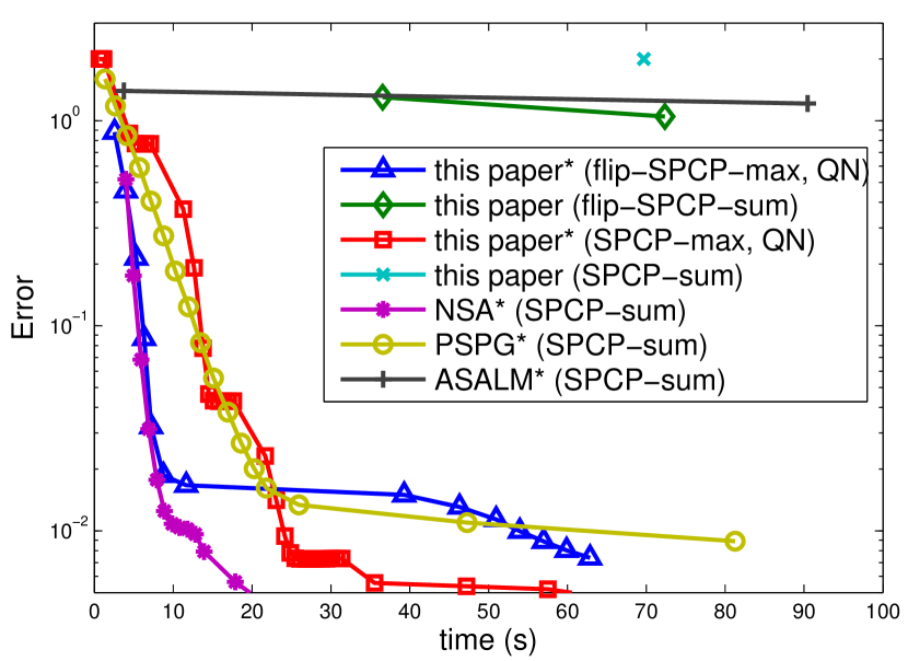
Figure 2: The $1500\times 1500$ synthetic noise test.

The results are shown in Fig. 2. Errors barely dip below $0.01$ (for comparison, an error of $2$ is achieved by setting $L=S=0$). The NSA and PSPG solvers do quite well. In contrast to the previous test, ASALM does poorly. Our methods for ($\text{flip-SPCP}_{\text{sum}}$), and hence ($\text{SPCP}_{\text{sum}}$), are not competitive, since they use dense SVDs. We imposed a time-limit of about one minute, so these methods only manage a single iteration or two. Our quasi-Newton method for ($\text{flip-SPCP}_{\text{max}}$) does well initially, then takes a long time due to a long partial SVD computation. Interestingly, ($\text{SPCP}_{\text{max}}$) does better than pure ($\text{flip-SPCP}_{\text{max}}$). One possible explanation is that it chooses a fortuitous sequence of $\tau$ values, for which the corresponding ($\text{flip-SPCP}_{\text{max}}$) subproblems become increasingly hard, and therefore benefit from the warm-start of the solution of the easier previous problem. This is consistent with empirical observations regarding continuation techniques, see e.g., (van den Berg & Friedlander, 2008; Wright et al., 2009b).

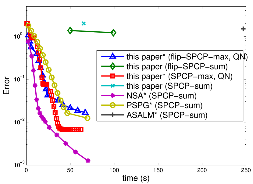
Figure 3: Second $1500\times 1500$ synthetic noise test.

Figure 3 is the same test but with $r=150$ and $p=0.1\cdot mn$, and the conclusions are largely similar.

7.3 Cloud removal

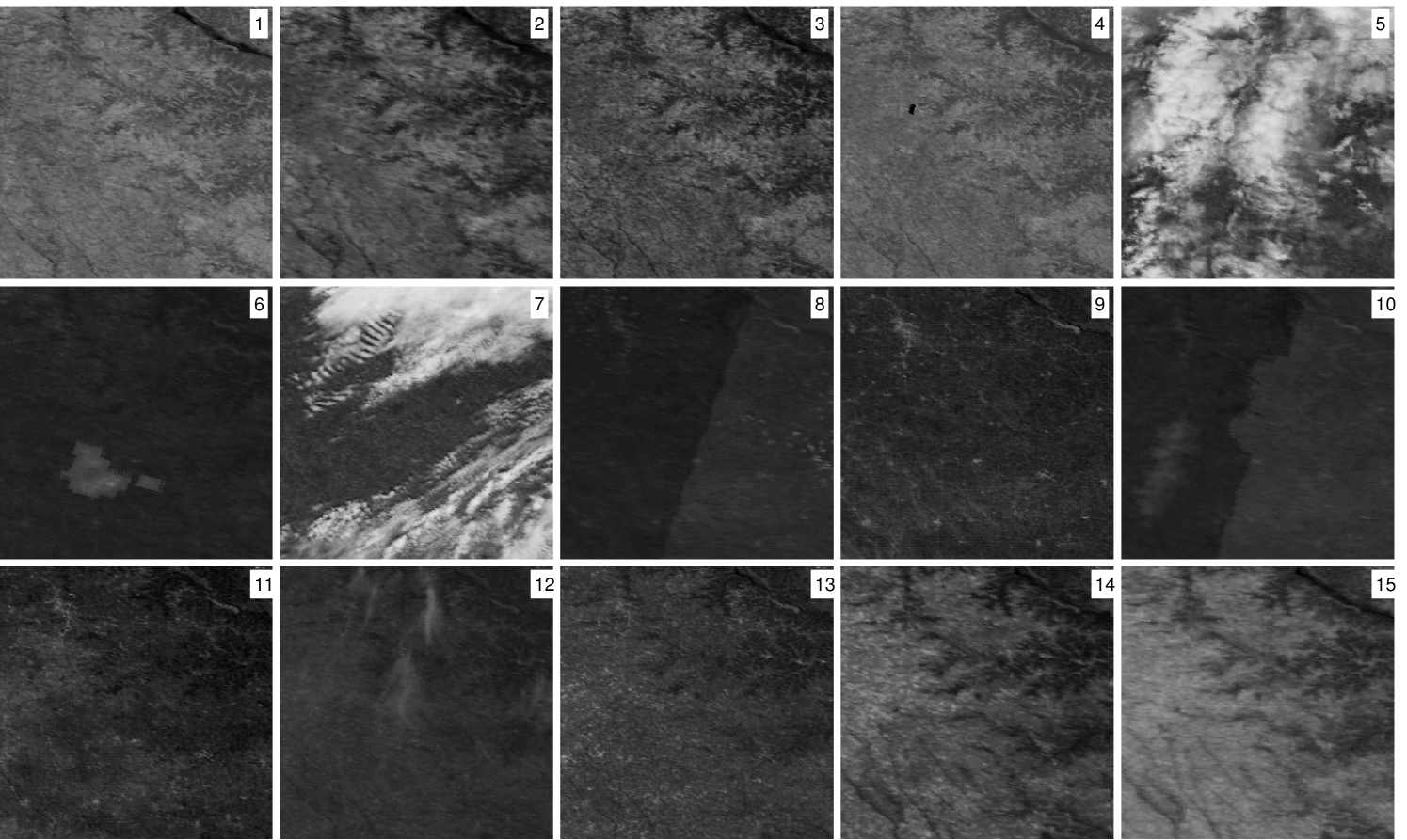
Figure 4: Satellite photos of the same location on different days

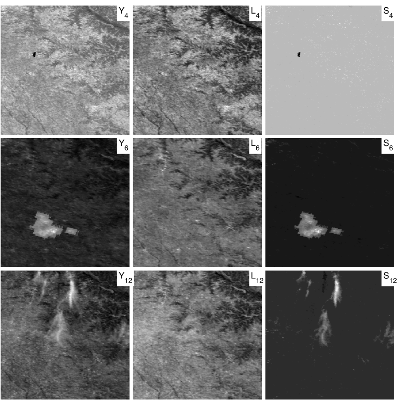
Figure 5: Showing frames 4, 5 and 12. Leftmost column is original data, middle column is low-rank term of the solution, and right column is sparse term of the solution. Data have been processed slightly to enhance contrast for viewing.

Figure 4 shows 15 images of size $300\times 300$ from the MODIS satellite, after some transformations to turn images from different spectral bands into one grayscale images. Each image is a photo of the same rural location but at different points in time over the course of a few months. The background changes slowly and the variability is due to changes in vegetation, snow cover, and different reflectance. There are also outlying sources of error, mainly due to clouds (e.g., major clouds in frames 5 and 7, smaller clouds in frames 9, 11 and 12), as well as artifacts of the CCD camera on the satellite (frame 4 and 6) and issues stitching together photos of the same scene (the lines in frames 8 and 10).

There are hundreds of applications for clean satellite imagery, so removing the outlying error is of great practical importance. Because of slow changing background and sparse errors, we can model the problem using the robust PCA approach. We use the ($\text{flip-SPCP}_{\text{max}}$) version due to its speed, and pick parameters $(\lambda_{\text{max}},\tau_{\text{max}})$ by using a Nelder-Mead simplex search. For an error metric to use in the parameter tuning, we remove frame $1$ from the data set (call it $y_{1}$) and set $Y$ to be frames 2–15. From this training data $Y$, the algorithm generates $L$ and $S$. Since $L$ is a $300^{2}\times 14$ matrix, it has far from full column span. Thus our error is the distance of $y_{1}$ from the span of $L$, i.e., $\|y_{1}-\mathcal{P}_{\text{span}(L)}(y_{1})\|_{2}$.

Our method takes about 11 iterations and 5 seconds, and uses a dense SVD instead of the randomized method due to the high aspect ratio of the matrix. Some results of the obtained $(L,S)$ outputs are in Fig. 5, where one can see that some of the anomalies in the original data frames $Y$ are picked up by the $S$ term and removed from the $L$ term. Frame 4 has what appears to be a camera pixel error; frame 6 has another artificial error (that is, caused by the camera and not the scene); and frame 12 has cloud cover.

8 CONCLUSIONS

In this paper, we reviewed several formulations and algorithms for the RPCA problem. We introduced a new denoising formulation ($\text{SPCP}_{\text{max}}$) to the ones previously considered, and discussed modeling and algorithmic advantages of denoising formulations ($\text{SPCP}_{\text{max}}$) and ($\text{SPCP}_{\text{sum}}$) compared to flipped versions ($\text{flip-SPCP}_{\text{max}}$) and ($\text{flip-SPCP}_{\text{sum}}$). In particular, we showed that these formulations can be linked using a variational framework, which can be exploited to solve denoising formulations using a sequence of flipped problems. For ($\text{flip-SPCP}_{\text{max}}$), we proposed a quasi-Newton acceleration that is competitive with state of the art, and used this innovation to design a fast method for ($\text{SPCP}_{\text{max}}$) through the variational framework. The new methods were compared against prior art on synthetic examples, and applied to a real world cloud removal application application using publicly available MODIS satellite data.

References

- Aravkin et al. (2013a) Aravkin, A. Y., Burke, J., and Friedlander, M. P. Variational properties of value functions. SIAM J. Optimization, 23(3):1689–1717, 2013a.
- Aravkin et al. (2013b) Aravkin, A. Y., Kumar, R., Mansour, H., Recht, B., and Herrmann, F. J. A robust SVD-free approach to matrix completion, with applications to interpolation of large scale data. 2013b. URL http://arxiv.org/abs/1302.4886.
- Aybat et al. (2013) Aybat, N., Goldfarb, D., and Ma, S. Efficient algorithms for robust and stable principal component pursuit. Computational Optimization and Applications, (accepted), 2013.
- Aybat & Iyengar (2014) Aybat, N. S. and Iyengar, G. An alternating direction method with increasing penalty for stable principal component pursuit. Computational Optimization and Applications, (submitted), 2014. http://arxiv.org/abs/1309.6553.
- Baldassarre et al. (2013) Baldassarre, L., Cevher, V., McCoy, M., Tran Dinh, Q., and Asaei, A. Convexity in source separation: Models, geometry, and algorithms. Technical report, 2013. http://arxiv.org/abs/1311.0258.
- Beck & Teboulle (2009) Beck, A. and Teboulle, M. A Fast Iterative Shrinkage-Thresholding Algorithm for Linear Inverse Problems. SIAM J. Imaging Sciences, 2(1):183–202, January 2009.
- Becker & Candès (2008) Becker, S. and Candès, E. Singular value thresholding toolbox, 2008. Available from http://svt.stanford.edu/.
- Brucker (1984) Brucker, P. An O(n) algorithm for quadratic knapsack problems. Operations Res. Lett., 3(3):163 – 166, 1984. doi: 10.1016/0167-6377(84)90010-5.
- Candès et al. (2011) Candès, E. J., Li, X., Ma, Y., and Wright, J. Robust principal component analysis? J. Assoc. Comput. Mach., 58(3):1–37, May 2011.
- Chandrasekaran et al. (2009) Chandrasekaran, V., Sanghavi, S., Parrilo, P. A., and Willsky, A. S. Sparse and low-rank matrix decompositions. In SYSID 2009, Saint-Malo, France, July 2009.
- Chandrasekaran et al. (2012) Chandrasekaran, V., Parrilo, P. A., and Willsky, A. S. Latent variable graphical model selection via convex optimization. Ann. Stat., 40(4):1935–2357, 2012.
- Chen et al. (2013) Chen, Caihua, He, Bingsheng, Ye, Yinyu, and Yuan, Xiaoming. The direct extension of admm for multi-block convex minimization problems is not necessarily convergent. Optimization Online, 2013.
- Combettes & Pesquet (2007) Combettes, P. L. and Pesquet, J.-C. A Douglas–Rachford Splitting Approach to Nonsmooth Convex Variational Signal Recovery. IEEE J. Sel. Topics Sig. Processing, 1(4):564–574, December 2007.
- Duchi et al. (2008) Duchi, J., Shalev-Shwartz, S., Singer, Y., and Chandra, T. Efficient projections onto the l1-ball for learning in high dimensions. In Intl. Conf. Machine Learning (ICML), pp. 272–279, New York, July 2008. ACM Press.
- Ganesh et al. (2009) Ganesh, A., Lin, Z., Wright, J., Wu, L., Chen, M., and Ma, Y. Fast algorithms for recovering a corrupted low-rank matrix. In Computational Advances in Multi-Sensor Adaptive Processing (CAMSAP), pp. 213–215, Aruba, Dec. 2009.
- Halko et al. (2011) Halko, N., Martinsson, P.-G., and Tropp, J. A. Finding structure with randomness: Probabilistic algorithms for constructing approximate matrix decompositions. SIAM review, 53(2):217–288, 2011.
- Huber (2004) Huber, P. J. Robust Statistics. John Wiley and Sons, 2 edition, 2004.
- Kyrillidis & Cevher (2014) Kyrillidis, Anastasios and Cevher, Volkan. Matrix recipes for hard thresholding methods. Journal of Mathematical Imaging and Vision, 48(2):235–265, 2014.
- Larsen (1998) Larsen, R. M. Lanczos bidiagonalization with partial reorthogonalization. Tech. Report. DAIMI PB-357, Department of Computer Science, Aarhus University, September 1998.
- Lee et al. (2010) Lee, J., Recht, B., Salakhutdinov, R., Srebro, N., and Tropp, J.A. Practical large-scale optimization for max-norm regularization. In Neural Information Processing Systems (NIPS), Vancouver, 2010.
- Lin et al. (2010) Lin, Z., Chen, M., and Ma, Y. The augmented Lagrange multiplier method for exact recovery of corrupted low-rank matrices. arXiv preprint arXiv:1009.5055, 2010.
- Mansour & Vetro (2014) Mansour, H. and Vetro, A. Video background subtraction using semi-supervised robust matrix completion. In To appear in IEEE International Conference on Acoustics, Speech, and Signal Processing (ICASSP), 2014.
- Peng et al. (2012) Peng, Y., Ganesh, A., Wright, J., Xu, W., and Ma, Y. RASL: Robust alignment by sparse and low-rank decomposition for linearly correlated images. IEEE Trans. Pattern Analysis and Machine Intelligence, 34(11):2233–2246, 2012.
- Recht & Ré (2011) Recht, Benjamin and Ré, Christopher. Parallel stochastic gradient algorithms for large-scale matrix completion. Math. Prog. Comput., pp. 1–26, 2011.
- Rockafellar (1970) Rockafellar, R. T. Convex analysis. Princeton Mathematical Series, No. 28. Princeton University Press, Princeton, N.J., 1970.
- Shen et al. (2014) Shen, Y., Wen, Z., and Zhang, Y. Augmented Lagrangian alternating direction method for matrix separation based on low-rank factorization. Optimization Methods and Software, 29(2):239–263, March 2014.
- Tao & Yuan (2011) Tao, M. and Yuan, X. Recovering low-rank and sparse components of matrices from incomplete and noisy observations. SIAM J. Optimization, 21:57–81, 2011.