Explorations of edge-weighted Cayley graphs and $p$-ary bent functions

Abstract

Let $f:GF(p)^{n}\rightarrow GF(p)$. When $p=2$, Bernasconi et al have shown that there is a correspondence between certain properties of $f$ (eg, if it is bent) and properties of its associated Cayley graph. Analogously, but much earlier, Dillon showed that $f$ is bent if and only if the “level curves” of $f$ had certain combinatorial properties (again, only when $p=2$). The attempt is to investigate an analogous theory when $p>2$ using the (apparently new) combinatorial concept of a weighted partial difference set. More precisely, we try to investigate which graph-theoretical properties of $\Gamma_{f}$ can be characterized in terms of function-theoretic properties of $f$, and which function-theoretic properties of $f$ correspond to combinatorial properties of the set of “level curves” $f^{-1}(a)$ ($a\in GF(p)$). While the natural generalizations of the Bernasconi correspondence and Dillon correspondence are not true in general, using extensive computations, we are able to determine a classification in small cases: $(p,n)\in\{(3,2),(3,3),(5,2)\}$. Our main conjecture is Conjecture 67.

1 Introduction

Fix $n\geq 1$ and let $V=GF(p)^{n}$, where $p$ is a prime.

Definition 1.

(Walsh(-Hadamard) transform) The Walsh(-Hadamard) transform of a function $f:GF(p)^{n}\rightarrow GF(p)$ is a complex-valued function on $V$ that can be defined as

$$W_{f}(u)=\sum_{x\in V}\zeta^{f(x)-\langle u,x\rangle},$$ (1)

where $\zeta=e^{2\pi i/p}$.

We call $f$ bent if

$$|W_{f}(u)|=p^{n/2},$$

for all $u\in V$. The class of $p$-ary bent functions are “maximally non-linear” in some sense, and can be used to generate pseudo-random sequences rather easily.

Some properties of the Walsh transform:

1. The Walsh coefficients satisfy Parseval’s equation

   $$\sum_{u\in V}|W_{f}(u)|^{2}=p^{2n}.$$

2. If $\sigma=\sigma_{k}:\mathbb{Q}(\zeta)\to\mathbb{Q}(\zeta)$ is defined by sending $\zeta\mapsto\zeta^{k}$ then $W_{f}(u)^{\sigma}=W_{kf}(ku)$.

If $f:V\to GF(p)$ then we let $f_{\mathbb{C}}:V\to\mathbb{C}$ be the function whose values are those of $f$ but regarded as integers (i.e., we select the congruence class residue representative in the interval $\{0,\dots,p-1\}$).

Definition 2.

(Fourier transform) When $f$ is complex-valued, we define the analogous Fourier transform of the function $f$ as

$$\hat{f}(y)=f^{\wedge}(y)=\sum_{x\in V}f_{\mathbb{C}}(x)\zeta^{-\langle x,y\rangle}.$$ (2)

Note

$$\hat{f}(0)=\sum_{x\in V}f_{\mathbb{C}}(x),$$

and note

$$W_{f}(y)=(\zeta^{f})^{\wedge}(y).$$

We say $f$ is even, if $f(-x)=f(x)$ for all $x\in GF(p)^{n}$. It is not hard to see that if $f$ is even then the Fourier transform of $f$ is real-valued. (However, this is not necessarily true of the Walsh transform.)

Example 3.

It turns out that there are a total of $3^{4}=81$ even functions $f:GF(3)^{2}\to GF(3)$ with $f(0)=0$, of which exactly $18$ are bent. Section 6.2 discusses this in more detail.

Example 4.

It turns out that there are a total of $3^{13}=1594323$ even functions $f:GF(3)^{3}\to GF(3)$ with $f(0)=0$, of which exactly $2340$ are bent. Section 6.3 discusses this in more detail.

Example 5.

It turns out that there are a total of $5^{12}=244140625$ even functions $f:GF(5)^{2}\to GF(5)$ with $f(0)=0$, of which exactly $1420$ are bent. Section 6.4 discusses this in more detail.

Definition 6.

(Hadamard matrix) We call an $N\times N$ $\{0,1\}$-matrix $M$ a Hadamard matrix if

$$M\cdot{M}^{t}=NI_{N},$$

where $I_{N}$ is the $N\times N$ identity matrix.

Remark 7.

There is a concept similar to the notion of bent, called “CAZAC.” We shall clarify their connection in this remark.

Constant amplitude zero autocorrelation (CAZAC) functions have been studied intensively since the 1990’s [BD]. We quote the following characterization, which is due to J. Benedetto and S. Datta [BD]:

Theorem: Given a sequence $x:\mathbb{Z}/N\mathbb{Z}\to\mathbb{C}$, and let $C_{x}$ be a circulant matrix with first row $x=(x[0],x[1],\dots,x[N-1])$. Then $x$ is a CAZAC sequence if and only if $C_{x}$ is a Hadamard matrix.

This is due to the fact that the definition of CAZAC functions uses the Fourier transform on $\mathbb{Z}/N\mathbb{Z}$. The corresponding definition of bent functions $f$ uses the Fourier transform (of $\zeta^{f}$) on $GF(p)^{n}$, $N=p^{n}$. The analogous Hadamard matrix for a bent function $f$ is not circulant but “block circulant.”

In the Boolean case, there is a nice simple relationship between the Fourier transform and the Walsh-Hadamard transform. In equation (24) below, we shall try to connect these two transforms, (1) and (2), in the $GF(p)$ case as well. In this context, it is worth noting that it is possible (see Proposition 73) to characterize a bent function in terms of the Fourier transform of its derivative.

Suppose $f:GF(p)^{n}\to GF(p)$ is bent.

Definition 8.

(regular) Suppose $f$ is bent. We say $f$ is regular if and only if $W_{f}(u)/p^{n/2}$ is a $p$th root of unity for all $u\in V$.

If $f$ is regular then there is a function $f^{*}:GF(p)^{n}\to GF(p)$, called the dual (or regular dual) of $f$, such that $W_{f}(u)=\zeta^{f^{*}(u)}p^{n/2}$, for all $u\in V$. We call $f$ weakly regular, if there is a function $f^{*}:GF(p)^{n}\to GF(p)$, called the dual (or $\mu$-regular dual) of $f$, such that $W_{f}(u)=\mu\zeta^{f^{*}(u)}p^{n/2}$, for some constant $\mu\in\mathbb{C}$ with absolute value $1$.

Proposition 9.

(Kumar, Scholtz, Welch) If $f$ is bent then there are functions $f_{*}:GF(p)^{n}\to\mathbb{Z}$ and $f^{*}:GF(p)^{n}\to GF(p)$ such that

$$W_{f}(u)p^{-n/2}=\left\{\begin{array}[]{rl}(-1)^{f_{*}(u)}\zeta^{f^{*}(u)},&{\rm if}\ n\ {\rm is\ even,\ or\ }n\ {\rm is\ odd\ and}\ p\equiv 1\pmod{4},\\ i^{f_{*}(u)}\zeta^{f^{*}(u)},&{\rm if}\ n\ {\rm is\ odd\ and}\ p\equiv 3\pmod{4}.\\ \end{array}\right.$$

The above result is known (thanks to Kumar, Scholtz, Welch [KSW]) but the form above is due to Helleseth and Kholosha [HK3] (although we made a minor correction to their statement). Also, note [KSW] Property 8 established a more general fact than the statement above.

Corollary 10.

If $f$ is bent and $W_{f}(0)$ is rational (i.e., belongs to $\mathbb{Q}$) then $n$ must be even.

The condition $W_{f}(0)\in\mathbb{Q}$ arises in Lemma 56 below, so this corollary shall be useful later.

Suppose $f:V=GF(p)^{n}\to GF(p)$ is bent. In this case, for each $u\in V$, the quotient $W_{f}(u)/p^{n/2}$ is an element of the cyclotomic field $\mathbb{Q}(\zeta)$ having absolute value $1$.

Below we give a simple necessary and sufficient conditions to determine if $f$ is regular. The next three lemmas are well-known but included for the reader’s convenience.

Lemma 11.

Suppose $f:V\to GF(p)$ is bent. The following are equivalent.

• $f$ is weakly regular.

• $W_{f}(u)/W_{f}(0)$ is a $p$-th root of unity for all $u\in V$.

Proof.

If $f$ is weakly regular with $\mu$-regular dual $f^{*}$, then $W_{f}(u)/W_{f}(0)=\zeta^{f^{*}(u)-f^{*}(0)}$, for each $u\in V$.

Conversely, if $W_{f}(u)/W_{f}(0)$ is of the form $\zeta^{i_{u}}$, for some integer $i_{u}$ (for $u\in V$), then let $f^{*}(u)$ be $i_{u}\pmod{p}$ and let $\mu=W_{f}(0)/(p^{n/2})$. Then $f^{*}(u)$ is a $\mu$-regular dual of $f$. $\Box$

Lemma 12.

Suppose $f:V\to GF(p)$ is bent and weakly regular. The following are equivalent.

• $f$ is regular.

• $W_{f}(0)/p^{n/2}$ is a $p$-th root of unity.

Proof.

One direction is clear. Suppose that $f$ is a weakly regular bent function with $\mu$-regular dual $f^{*}$ and suppose that $W_{f}(0)/(p^{n/2})=\zeta^{i}$. Note that $W_{f}(0)=\mu\zeta^{f*(0)}p^{n/2}=\zeta^{i}p^{n/2}$ so that $\mu=\zeta^{i-f*(0)}$. Let $g(u)=f^{*}(u)-f^{*}(0)+i$ (where we are treating $i$ as an element of $GF(p)$). Then

$$W_{f}(u)=\mu\zeta^{f*(u)}p^{n/2}=\zeta^{i-f^{*}(0)}\zeta^{g(u)+f^{*}(0)-i}p^{n}/2=\zeta^{g(u)}p^{n/2},$$

so $f$ is regular. $\Box$

Lemma 13.

Suppose that $f$ is bent and weakly regular, with $\mu$-regular dual $f^{*}$. Then $f^{*}$ is bent and weakly regular, with $\mu^{-1}$-regular dual $f^{**}$ given by $f^{**}(x)=f(-x)$. If $f$ is also even, then $f^{*}$ is even and $f^{**}=f$.

Proof.

Suppose that $f$ is bent and weakly regular with $\mu$-regular dual $f^{*}$. Then

$$W_{f}(u)=\mu\zeta^{f^{*}(u)}p^{\frac{n}{2}}$$

for all $u$ in $V$. The Walsh transform of $f^{*}$ is given by

$$W_{f^{*}}(u) =\sum_{y\in V}\zeta^{f^{*}(y)}\zeta^{-\langle u,y\rangle}$$ (3)

$$=\sum_{y\in V}\mu^{-1}p^{-\frac{n}{2}}W_{f}(y)\zeta^{-\langle u,y\rangle}$$

$$=\mu^{-1}p^{-\frac{n}{2}}\sum_{y\in V}\sum_{x\in V}\zeta^{f(x)}\zeta^{-\langle y,x\rangle}\zeta^{-\langle u,y\rangle}$$

$$=\mu^{-1}p^{-\frac{n}{2}}\sum_{y\in V}\sum_{x\in V}\zeta^{f(x)}\zeta^{-\langle y,x+u\rangle}$$

$$=\mu^{-1}p^{-\frac{n}{2}}\sum_{w\in V}\zeta^{f(w-u)}\sum_{y\in V}\zeta^{-\langle y,w\rangle}.$$

Next we note that

$$\sum_{y\in V}\zeta^{-\langle y,w\rangle}=\begin{cases}p^{n}&\text{if }w=0\\ 0&\text{if }w\neq 0\end{cases}$$

since, if $y=(y_{1},y_{2},\ldots,y_{n})$ and $w=(w_{1},w_{2},\ldots,w_{n})$, we have

$$\sum_{y\in V}\zeta^{-\langle y,w\rangle} =\sum_{y_{1}\in GF(p)}\sum_{y_{2}\in GF(p)}\ldots\sum_{y_{n}\in GF(p)}\zeta^{-y_{1}w_{1}}\zeta^{-y_{2}w_{2}}\ldots\zeta^{-y_{n}w_{n}}$$

$$=\prod_{i=1}^{n}\left(\sum_{y\in GF(p)}\zeta^{-yw_{i}}\right)$$

and, if $w_{i}\neq 0$,

$$\sum_{y\in GF(p)}\zeta^{-yw_{i}}=\zeta^{0}+\zeta^{1}+\ldots+\zeta^{p-1}=0.$$

Therefore equation 3 reduces to

$$W_{f^{*}}(u) =\mu^{-1}p^{-\frac{n}{2}}\zeta^{f(-u)}p^{n}$$

$$=\mu^{-1}\zeta^{f(-u)}p^{\frac{n}{2}}.$$

It follows that $f^{*}$ is bent with $\mu^{-1}$-regular dual $f^{**}$ given by $f^{**}(x)=f(-x)$ and that if $f$ is even, $f^{**}=f$.

Furthermore, if $f$ is even,

$$\zeta^{f^{*}(-u)} =\mu^{-1}p^{-\frac{n}{2}}W_{f}(-u)$$

$$=\mu^{-1}p^{-\frac{n}{2}}\sum_{x\in V}\zeta^{f(x)}\zeta^{-\langle-u,x\rangle}$$

$$=\mu^{-1}p^{-\frac{n}{2}}\sum_{w\in V}\zeta^{f(-w)}\zeta^{-\langle u,w\rangle}$$

$$=\mu^{-1}p^{-\frac{n}{2}}\sum_{w\in V}\zeta^{f(w)}\zeta^{-\langle u,w\rangle} f$$ since is even

$$=\mu^{-1}p^{-\frac{n}{2}}W_{f}(u)$$

$$=\zeta^{f^{*}(u)}.$$

Since $f^{*}$ takes values in $GF(p)$, it follows that $f^{*}(-u)=f^{*}(u)$ for all $u$ in $V$, so $f^{*}$ is even. $\Box$

2 Partial difference sets

Dillon’s thesis [D] was one of the first publications to discuss the relationship between bent functions and combinatorial structures, such as difference sets. His work concentrated on the Boolean case. Consider functions

$$f:GF(p)^{n}\to GF(p),$$

where $p$ is a prime, $n>1$ is an integer. In Dillon’s work, it was proven that the “level curve” $f^{-1}(1)$ gives rise to a difference set in $GF(2)^{n}$.

Definition 14.

(difference set) Let $G$ be a finite abelian multiplicative group of order $v$, and let $D$ be a subset of $G$ with order $k$. $D$ is a $(v,k,\lambda)$-difference set (DS) if the list of differences $d_{1}d_{2}^{-1},d_{1},d_{2}\in D$, represents every non-identity element in $G$ exactly $\lambda$ times.

A Hadamard difference set is one whose parameters are of the form $(4m^{2},2m^{2}-m,m^{2}-m)$, for some $m>1$. It is, in addition, elementary if $G$ is an elementary abelian $2$-group (i.e., isomorphic to $(\mathbb{Z}/2\mathbb{Z})^{n}$).

Let $D^{-1}=\{d^{-1}\ |\ d\in D\}$.

Lemma 15.

Let $G$ be a finite abelian multiplicative group of order $v$ and let $D$ be a subset of $G$ with order $k$, such that $D=D^{-1}$. If $(G,D)$ is an $(v,k,\lambda,\lambda)$-partial difference set then it is also a $(v,k,\lambda)$-difference set.

Proof.

This follows from character theory: combine Theorem 1 and Theorem 2, and (the proof of) Proposition 1 in Polhill [Po]. $\Box$

Theorem 16.

(Dillon Correspondence, [D], Theorem 6.2.10, page 78) The function $f:GF(2)^{n}\to GF(2)$ is bent if and only if $f^{-1}(1)$ is an elementary Hadamard difference set of $GF(2)^{n}$.

Two (naive) analogs of this are formalized below in Analog 34 and Analog 35.

2.1 Weighted partial difference sets

In this paper, we consider the “level curves” $f^{-1}(a)\subset GF(p)^{n}$ ($a\in GF(p)$, $a\not=0$) and investigate the combinatorial structure of these sets, especially when $f$ is bent.

Definition 17.

(PDS) Let $G$ be a finite abelian multiplicative group of order $v$, and let $D$ be a subset of $G$ with order $k$. $D$ is a $(v,k,\lambda,\mu)$-partial difference set (PDS) if the list of differences $d_{1}d_{2}^{-1},d_{1},d_{2}\in D$, represents every non-identity element in $D$ exactly $\lambda$ times and every non-identity element in $G\setminus D$ exactly $\mu$ times.

This notion can be characterized algebraically in terms of the group ring $\mathbb{C}[G]$.

Lemma 18.

With the notation as in the defintion above, $(G,D)$ forms a $(v,k,\lambda,\mu)$-PDS if and only if (6) holds.

The well-known proof is omitted.

Example 19.

Consider the finite field

$$GF(9)=GF(3)[x]/(x^{2}+1)=\{0,1,2,x,x+1,x+2,2x,2x+1,2x+2\},$$

written additively. The set of non-zero quadratic residues is given by

$$D=\{1,2,x,2x\}.$$

One can show that $D$ is a PDS with parameters

$$v=9,\ \ k=4,\ \ \lambda=1,\ \ \mu=2.$$

We shall return to this example (with more details) below, in Example 26.

Definition 20.

(Latin square type PDS) Let $(G,D)$ be a PDS. We say it is of Latin square type (resp., negative Latin square type) if there exist $N>0$ and $R>0$ (resp., $N<0$ and $R<0$) such that

$$(v,k,\lambda,\mu)=(N^{2},R(N-1),N+R^{2}-3R,R^{2}-R).$$

The example above is of Latin square type ($N=3$ and $R=2$) and of negative Latin square type ($N=-3$ and $R=-1$).

Let $G$ be a finite abelian multiplicative group and let $D$ be a subset of $G$. Decompose $D$ into a union of disjoint subsets

$$D=D_{1}\cup\dots\cup D_{r},$$ (4)

and assume $1\notin D$. Let $k_{i}=|D_{i}|$.

Definition 21.

(weighted PDS) Let $W$ be a weight set of size $r$, and $v\in\mathbb{Z}$, $k\in\mathbb{Z}^{|W|}$, $\lambda\in\mathbb{Z}^{|W^{3}|}$, and $\mu\in\mathbb{Z}^{|W^{2}|}$. We say $D$ is a weighted $(v,k,\lambda,\mu)$-PDS, if the following properties hold

• The list of “differences”

  $$D_{i}D_{j}^{-1}=\{d_{1}d_{2}^{-1}\ |\ d_{1}\in D_{i},d_{2}\in D_{j}\},$$

  represents every non-identity element of $D_{\ell}$ exactly $\lambda_{i,j,\ell}$ times and every non-identity element of $G\setminus D$ exactly $\mu_{i,j}$ times ($1\leq i,j,\ell\leq r$).

• For each $i$ there is a $j$ such that $D_{i}^{-1}=D_{j}$ (and if $D_{i}^{-1}=D_{i}$ for all $i$ then we say the weighted PDS is symmetric).

This notion can be characterized algebraically in terms of the group ring $\mathbb{C}[G]$.

Lemma 22.

With the notation as in the definition above, $(G,D_{1},\dots,D_{s})$ forms a symmetric weighted $(v,k,\lambda,\mu)$-PDS if and only if $D=D^{-1}$ and (21) holds.

The straightforward proof is omitted.

Remark 23.

If $D=D_{1}\cup\dots\cup D_{r}$ is a symmetric weighted PDS then $\mu_{i,j}=\mu_{j,i}$ and $\lambda_{i,j,\ell}=\lambda_{j,i,\ell}$.

How does the above notion of a weighted PDS relate to the usual notion of a PDS?

Lemma 24.

Let $(G,D)$, where $D=D_{1}\cup\dots\cup D_{r}$ (disjoint union) is as in (4), be a symmetric weighted PDS, with parameters $(v,(k_{i}),(\lambda_{i,j,\ell}),(\mu_{i,j}))$. If

$$\sum_{i,j}\lambda_{i,j,\ell}$$

does not depend on $\ell$, $1\leq\ell\leq r$, then $D$ is also an unweighted PDS with parameters $(v,k,\lambda,\mu)$ where

$$k=\sum_{i}k_{i},\ \ \lambda=\sum_{i,j}\lambda_{i,j,\ell},\ \ \ \ \mu=\sum_{i,j}\mu_{i,j}.$$

Remark 25.

Case 1 in Proposition 91 does not satisfy this hypothesis.

Proof.

The claim is that $(G,D)$ is a PDS with parameters $(v,k,\lambda,\mu)$. Since $v=|G|$ and

$$k=|D|=|D_{1}|+\dots+|D_{r}|=k_{1}+\dots+k_{r},$$

we need only verify the claim regarding $\lambda$ and $\mu$.

Does each element $d$ of $D$ occur the same number of times in the list $DD^{-1}$? Suppose $d\in D_{\ell}$, where $1\leq\ell\leq r$. By hypothesis, $d$ occurs in $D_{i}-D_{j}$ exactly $\lambda_{i,j,\ell}$ times. Since $DD^{-1}$ is the concatenation of the $D_{i}D_{j}^{-1}$, for $1\leq i,j\leq r$, $d$ occurs in $D\cdot D^{-1}$ exactly

$$\sum_{i,j}\lambda_{i,j,\ell}$$

times. By hypothesis, this does not depend on $\ell$, so the claim regarding $\lambda$ has been verified.

Does each non-zero element $d$ of $G\setminus D$ occur the same number of times in the list $D\cdot D^{-1}$? By hypothesis, $d$ occurs in $D_{i}D_{j}^{-1}$ exactly $\mu_{i,j}$ times. Since $D\cdot D^{-1}$ is the concatenation of the $D_{i}D_{j}^{-1}$, for $1\leq i,j\leq r$, $d$ occurs in $D\cdot D^{-1}$ exactly

$$\sum_{i,j}\mu_{i,j}$$

times. This verifies the claim regarding $\mu$ and completes the proof of the lemma.

$\Box$

Example 26.

Consider the finite field

$$GF(9)=GF(3)[x]/(x^{2}+1)=\{0,1,2,x,x+1,x+2,2x,2x+1,2x+2\},$$

written multiplicatively The set of non-zero quadratic residues is given by

$$D=\{1,2,x,2x\}.$$

Let $D_{1}=\{1,2\}$ and $D_{2}=\{x,2x\}$.

Translating the multiplicative notation to the additive notation, we find

$$D_{1}D_{1}^{-1}=[d_{1}-d_{2}\ |\ d_{1}\in D_{1},d_{2}\in D_{1}]=[0,0,1,2],$$

$$D_{1}D_{2}^{-1}=[d_{1}-d_{2}\ |\ d_{1}\in D_{1},d_{2}\in D_{2}]=[x+1,x+2,2x+1,2x+2],$$

$$D_{2}D_{1}^{-1}=[d_{1}-d_{2}\ |\ d_{1}\in D_{2},d_{2}\in D_{1}]=[x+1,x+2,2x+1,2x+2],$$

$$D_{2}D_{2}^{-1}=[d_{1}-d_{2}\ |\ d_{1}\in D_{2},d_{2}\in D_{2}]=[0,0,x,2x].$$

Therefore, this describes a weighted PDS with parameters

$$k_{1,1}=2,\ k_{2,2}=2,\ k_{1,2}=k_{2,1}=0,$$

$$\lambda_{1,1,1}=1,\ \lambda_{1,1,2}=0,\ \lambda_{1,2,1}=0,\ \lambda_{1,2,2}=0,\$$

$$\lambda_{2,1,1}=0,\ \lambda_{2,1,2}=0,\ \lambda_{2,2,1}=0,\ \lambda_{2,2,2}=1,$$

and

$$\mu_{1,1}=0,\ \mu_{1,2}=1,\ \mu_{2,1}=1,\ \mu_{2,2}=0.$$

As we will see, there a weighted analog of the correspondence between PDSs and SRGs.

We have the following generalization of Theorem 42.

Theorem 27.

Let $G$ be an abelian multiplicative group and let $D\subset G$ be a subset such that $1\notin D$ and with disjoint decomposition $D=D_{1}\cup D_{2}\cup\dots\cup D_{r}$. The following are equivalent:

• $(G,D)$ is a symmetric weighted partial difference set having parameters $(v,k,\lambda,\mu)$, where $v=|G|$, $k=\{k_{i}\}$ with $k_{i}=|D_{i}|$, $\lambda=\{\lambda_{i,j,\ell}\}$, and $\mu=\{\mu_{i,j}\}$.

• $\Gamma(G,D)$ is a strongly regular edge-weighted (undirected) graph with parameters $(v,k,\lambda,\mu)$ as in (a).

Proof.

Let $D^{\prime}=G\setminus D-\{1\}$.

((a) $\implies$ (b)) Suppose $(G,D)$ is a weighted partial difference set satisfying $D_{i}=D_{i}^{-1}$, for all $i$. The graph $\Gamma=\Gamma(G,D)$ has $v=|G|$ vertices, by definition. Each vertex $g$ of $\Gamma$ has $k_{i}$ neighbors of weight $i$, namely, $dg$ where $d\in D_{i}$. (We say two vertices are “neighbors having edge-weight $0$” if they are not connected by an edge in the unweighted graph.) Let $g_{1},g_{2}$ be distinct vertices in $\Gamma$. Let $x$ be a vertex which is a neighbor of each: $x\in N(g_{1},i)\cap N(g_{2},j)$. By definition, $x=d_{1}g_{1}=d_{2}g_{2}$, for some $d_{1}\in D_{i}$, $d_{2}\in D_{j}$. Therefore, $d_{1}^{-1}d_{2}=g_{1}g_{2}^{-1}$. If $g_{1}g_{2}^{-1}\in D_{\ell}$, for some $\ell\not=0$, then there are $\lambda_{i,j,\ell}$ solutions, by definition of a weighted PDS. If $g_{1}g_{2}^{-1}\in D^{\prime}$ then there are $\mu_{i,j}$ solutions, by definition of a weighted PDS.

((b) $\implies$ (a)) Note $f$ even implies the symmetric condition of a weighted PDS. For the remainder of the proof, note the reasoning above is reversible. Details are left to the reader. $\Box$

Let $f$ be a $GF(p)$-valued function on $V$. The Cayley graph of $f$ is defined to be the edge-weighted digraph

$$\Gamma_{f}=(GF(p)^{n},E_{f}),$$ (5)

whose vertex set is $V=V(\Gamma_{f})=GF(p)^{n}$ and the set of edges is defined by

$$E_{f}=\{(u,v)\in GF(p)^{n}\ |\ f(u-v)\not=0\},$$

where the edge $(u,v)\in E_{f}$ has weight $f(u-v)$. However, if $f$ is even then we can (and do) regard $\Gamma_{f}$ as a weighted (undirected) graph.

Theorem 28.

Let $f:GF(p)^{n}\rightarrow GF(p)$ be an even function such that $f(0)=0.$ Let $D_{i}=f^{-1}(i)$, for $i=1,2,\dots,p-1$, and $D_{0}=\{0\}$. Let $D_{p}=GF(p)^{n}\setminus D_{0}\cup D_{1}\cup\cdots\cup D_{p-1}.$ If $(GF(p)^{n},D_{0},\dots,D_{p})$ is a weighted partial difference set, where $G=GF(p)^{n}$, then the associated (strongly regular) graph is the (edge-weighted) Cayley graph of $f$.

Remark 29.

Roughly speaking, this theorem says that “if the level curves of $f$ form a weighted PDS then the (edge-weighted) Cayley graph corresponding to $f$ agrees with the (edge-weighted) strongly regular graph associated to the weighted PDS.”

Proof.

The adjacency matrix $A$ for the Cayley graph of $f$ is defined by $A_{ij}=f(j-i)$ for $i,j\in GF(p)^{n}$. So the top row of A is defined by $A_{0j}=f(j)$. The adjacency matrix for any Cayley graph can be determined from its top row, since it is a circulant matrix. Therefore, it is enough to show that that the adjacency matrix of the weighted partial difference set has the same top row as $A$. Let $B$ be the adjacency matrix of the weighted partial difference set. Then $B$ is defined by $B_{ij}=k$ if $j-i\in D_{k}$ (for all $i,j\in GF(p)^{n}$ and $k\in GF(p)$). The top row of $B$ is defined by $B_{0j}=k$ if $j\in D_{k}$. But if $j\in D_{k}$, then $f(j)=k$, so $B_{0j}=f(j)$. The top rows of $A$ and $B$ are equivalent, so $A=B$. Therefore, the strongly regular graph associated with the weighted partial difference set $(G,D)$ is the Cayley graph of $f$. $\Box$

Conjecture 30.

(Walsh) If $f:GF(p)^{n}\to GF(p)$, $p>2$ is weakly regular and bent and corresponds to a weighted SRG (via Analog 61) then $\mu_{ii}=0$, $1\leq i\leq s$, for the associated weighted PDS.

Remark 31.

If you drop the hypothesis that $f$ be weakly regular then the conjecture is false.

2.2 Association schemes

The following definition is standard, but we give [PTFL] as a reference.

Definition 32.

(association scheme) Let $S$ be a finite set and let $R_{0},R_{1},\dots,R_{s}$ denote binary relations on $S$ (subsets of $S\times S$). The dual of a relation $R$ is the set

$$R^{*}=\{(x,y)\in S\times S\ |\ (y,x)\in R\}.$$

Assume $R_{0}=\Delta_{S}=\{(x,x)\in S\times S\ |\ x\in S\}$. We say $(S,R_{0},R_{1},\dots,R_{s})$ is a $s$-class association scheme on $S$ if the following properties hold.

• We have a disjoint union

  $$S\times S=R_{0}\cup R_{1}\cup\dots\cup R_{s},$$

  with $R_{i}\cap R_{j}=\emptyset$ for all $i\not=j$.

• For each $i$ there is a $j$ such that $R_{i}^{*}=R_{j}$ (and if $R_{i}^{*}=R_{i}$ for all $i$ then we say the association scheme is symmetric).

• For all $i,j$ and all $(x,y)\in S\times S$, define

  $$p_{ij}(x,y)=|\{z\in S\ |\ (x,z)\in R_{i},(z,y)\in R_{j}\}|.$$

  For eack $k$, and for all $x,y\in R_{k}$, the integer $p_{ij}(x,y)$ is a constant, denoted $p_{ij}^{k}$.

These constants $p_{ij}^{k}$ are called the intersection numbers or parameters or structure constants of the association scheme.

Next, we recall (see Herman [He]) the matrix-theoretic version of this definition.

Definition 33.

(adjacency ring) Let $S$ be a finite abelian multiplicative group of order $m$. Let $(S,R_{0},\dots,R_{s})$ denote a tuple consisting of $S$ with relations $R_{i}$ for which we have a disjoint union

$$S\times S=R_{0}\cup R_{1}\cup\dots\cup R_{s},$$

with $R_{i}\cap R_{j}=\emptyset$ for all $i\not=j$. Let $A_{i}\in Mat_{m\times m}(\mathbb{Z})$ denote the adjacency matrix of $R_{i}$, $i=0,1,\dots,s$.

We say that the subring of $\mathbb{Z}[Mat_{m\times m}(\mathbb{Z})]$ is an adjacency ring (also called the Bose-Mesner algebra) provided the set of adjacency matrices satisfying the following five properties:

• for each integer $i\in[0,\dots,s]$, $A_{i}$ is a $(0,1)$-matrix,

• $\sum_{i=0}^{s}A_{i}=J$ (the all $1$’s matrix),

• for each integer $i\in[0\dots,s]$, ${}^{t}A_{i}=A_{j}$, for some integer $j\in[0,s]$,

• there is a subset $J\subset G$ such that $\sum_{j\in J}A_{j}=I$, and

• there is a set of non-negative integers $\{p_{ij}^{k}\ |\ i,j,k\in[0,\dots,s]\}$ such that equation (20) holds for all such $i,j$.

Regarding the Dillon correspondence, we have the following combinatorial analogs (which may or may not be true in general).

Analog 34.

If $f$ is an even bent function then the tuple

$$(GF(p)^{n},D_{0},D_{1},D_{2},\cdots,D_{p-1},D_{p})$$

defines a weighted partial difference set.

We reformulate this in an essentially equivalent way using the language of association schemes.

Analog 35.

Let $f$ be as above and let $R_{0},R_{1},\dots,R_{p}$ denote binary relations on $GF(p)^{n}$ given by

$$R_{i}=\{(x,y)\in GF(p)^{n}\times GF(p)^{n}\ |\ f(x,y)=i\},\ \ \ 0\leq i\leq p.$$

If $f$ is an even bent function then $(GF(p)^{n},R_{0},R_{1},\dots,R_{p})$ is a $p$-class association scheme.

It is well-known that a PDS $(G,D)$ is naturally associated to a $2$-class association scheme, namely $(G,R_{0},R_{1},R_{2})$ where

$$R_{0}=\Delta_{G},$$

$$R_{1}=\{(g,h)\ |\ gh^{-1}\in D\},$$

$$R_{2}=\{(g,h)\ |\ gh^{-1}\notin D,\ g\not=h\}.$$

To verify this, let consider the “Schur ring.”

For the following definition, we identify any subset $S$ of $G$ with the formal sum of its elements in $\mathbb{C}[G]$.

Definition 36.

(Schur ring) Let $G$ be a finite abelian group and let $C_{0},C_{1},\dots,C_{s}$ denote finite subsets with the following properties.

• $C_{0}=\{1\}$ is the singleton containing the identity.

• We have a disjoint union

  $$G=C_{0}\cup C_{1}\cup\dots\cup C_{s},$$

  with $C_{i}\cap C_{j}=\emptyset$ for all $i\not=j$.

• for each $i$ there is a $j$ such that $C_{i}^{-1}=C_{j}$ (and if $C_{i}^{-1}=C_{i}$ for all $i$ then we say the Schur ring is symmetric).

• for all $i,j$, we have

  $$C_{i}\cdot C_{j}=\sum_{k=0}^{s}\rho_{ij}^{k}C_{k},$$

  for some integers $\rho_{ij}^{k}$.

The subalgebra of $\mathbb{C}[G]$ generated by $C_{0},C_{1},\dots,C_{s}$ is called a Schur ring over $G$.

In the cases we are dealing with, the Schur ring is commutative, so $\rho_{ij}^{k}=\rho_{ji}^{k}$, for all $i,j,k$.

If $(G,C_{0},\dots,C_{s})$ is a Schur ring then

$$R_{i}=\{(g,h)\in G\times G\ |\ gh^{-1}\in C_{i}\},$$

for $0\leq i,j\leq s$, gives rise to its corresponding association scheme.

Remark 37.

Weighted PDSs in the notation of Definition 21 naturally correspond to association schemes of class $r+1$. For a precise version of this, see Proposition 70 below.

Example 38.

For an example of a Schur ring, we return to the PDS, $(G,D)$. Let

$$D^{\prime}=G\setminus(D\cup\{1\}).$$

We have the well-known intersection

$$\begin{array}[]{rl}D\cdot D&=(k-\mu)\cdot I+(\lambda-\mu)\cdot D+\mu\cdot G\\ &=k\cdot I+\lambda\cdot D+\mu\cdot D^{\prime}\ ,\\ \end{array}$$ (6)

and

$$\begin{array}[]{rl}D\cdot D^{\prime}&=(-k+\mu)\cdot 1+(-1-\lambda+\mu)\cdot D+(k-\mu)\cdot G\\ &==0\cdot I+(k-1-\lambda)\cdot D+(k-\mu)\cdot D^{\prime}\ .\\ \end{array}$$ (7)

Provided $k\geq{\rm max}(\mu,\lambda+1)$, $|G|\geq{\rm max}(k+1,2k-\mu+2)$, with these, one can verify that a PDS naturally yields an associated Schur ring, generated by $D$, $D^{\prime}$, and $D_{0}=\{1\}$ in $\mathbb{C}[G]$, and a $2$-class association scheme.

Using (7), one can verify that $D^{\prime}$ is $(v,k^{\prime},\lambda^{\prime},\mu^{\prime})$-PDS with $(D^{\prime})^{-1}=D^{\prime}$ and $1\notin D^{\prime}$, where

$$\begin{array}[]{rl}k^{\prime}&=v-k-1\\ \lambda^{\prime}&=v-2k-2+\mu,\rm{and}\\ \mu^{\prime}&=v-2k+\lambda.\end{array}$$ (8)

.

We include a proof here for convenience.

Proof.

We will show that $D^{\prime}$ is a $(v,k^{\prime},\lambda^{\prime},\mu^{\prime})$-partial difference set. The first of these three equations is immediate, from the definition of $D^{\prime}$. The fact that $D^{\prime}=(D^{\prime})^{-1}$ also follows immediately the hypotheses.

By the definition of $D$, and because $D^{-1}=D$, we have

$$D\cdot D=k{1}+\lambda D+\mu D^{\prime}.$$ (9)

To find $D\cdot D^{\prime}$, we note that

$$\begin{array}[]{rl}kG&=D\cdot G\\ &=D\cdot(\{1\}+D+D^{\prime})\\ &=D+D\cdot D+D\cdot D^{\prime}\end{array}$$

so that

$$D\cdot D^{\prime}=(k-\lambda-1)D+(k-\mu)D^{\prime}.$$ (10)

Similarly, we note that

$$\begin{array}[]{rl}k^{\prime}G&=G\cdot D^{\prime}\\ &=((\{1\}+D+D^{\prime})\cdot D^{\prime}\\ &=D^{\prime}+D\cdot D^{\prime}+D^{\prime}\cdot D^{\prime}\end{array}$$

so that

$$\begin{array}[]{rl}D^{\prime}\cdot D^{\prime}&=k^{\prime}\{1\}+(k^{\prime}-k+\lambda+1)D+(k^{\prime}-k-1-+\mu)D^{\prime}\\ &=k^{\prime}\{1\}+(v-2k+\lambda)D+(v-2k-2+\mu)D^{\prime}.\end{array}$$ (11)

Equation 11 shows that $D^{\prime}$ is a $(v,k^{\prime},\lambda^{\prime},\mu^{\prime})$-partial difference set, with $\lambda^{\prime}$ and $\mu^{\prime}$ as in Equation 8.

$\Box$

It can be shown that $\mu^{\prime}=k^{\prime}\left(1-\frac{\mu}{k}\right).$

With the identities in the above example, one can verify that a PDS naturally yields an associated Schur ring and a $2$-class association scheme.

We will now state a more general proposition concerning weighted partial difference sets.

Proposition 39.

Let $G$ be a finite abelian group. Let $D_{0},\cdots,D_{r}\subseteq G$ such that $D_{i}\cap D_{j}=\emptyset$ if $i\neq j$, and

• $G$ is the disjoint union $D_{0}\cup\cdots\cup D_{r}$

• for each $i$ there is a $j$ such that $D_{i}^{-1}=D_{j}$, and

• $D_{i}\cdot D_{j}=\sum\limits_{k=0}^{r}p_{ij}^{k}D_{k}$ for some positive integer $p_{ij}^{k}$.

Then the matrices $P_{k}=(p_{ij}^{k})_{0\leq i,j\leq l}$ satisfy the following properties:

• $P_{0}$ is a diagonal matrix with entries $|D_{0}|,\cdots,|D_{r}|$

• For each $k$, the $j$th column of $P_{k}$ has sum $|D_{j}|$ ($j=0,\cdots,l$). Likewise, the $i$th row of $P_{k}$ has sum $|D_{i}|$ ($i=0,\cdots,l$).

Proof.

We begin by taking the sum

$D_{i}\cdot D_{j}=\sum\limits_{k=0}^{r}p_{ij}^{k}D_{k}$

over all $i,0\leq i\leq l$.

$G\cdot D_{j}=\sum\limits_{k=0}^{r}(\sum\limits_{i=0}^{r}p_{ij}^{k})D_{k}$

We know that $G\cdot D_{j}=|D_{j}|\cdot G$, and all the $D_{k}$ are disjoint. As an identity in the Schur ring, each element of G must occur $|D_{j}|$ times on each side of this equation. Therefore,

$|D_{j}|=\sum\limits_{i=0}^{r}p_{ij}^{k}$.

So the sum of the elements in the $j$th row of $P_{k}$ is $|D_{j}|$ for each $j$ and $k$. The analogous claim for the row sums is proven similarly. $\Box$

3 Cayley graphs

Let $(G,D)$ be a PDS.

Definition 40.

(Cayley graph) The Cayley graph $\Gamma=\Gamma(G,D)$ associated to the PDS $(G,D)$ is a graph constructed as follows: from a subset $D$ of $G$, let the vertices of the graph be the elements of the group $G$. Two vertices $g_{1}$ and $g_{2}$ are connected by a directed edge if $g_{2}=dg_{1}$ for some $d\in D$.

If $D$ is a partial difference set such that $\lambda\not=\mu$, then $D=D^{-1}$ (Proposition 1 in [Po]). Thus, if $g_{2}=dg_{1}$, then $g_{1}=d^{-1}g_{2}$, so the Cayley graph $\Gamma(G,D)$ is an undirected graph.

Definition 41.

(SRG) A connected graph $\Gamma=(V,E)$ is a $(v,k,\lambda,\mu)$-strongly regular graph if:

• $\Gamma$ has $v$ vertices such that each vertex is connected to $k$ other vertices

• Distinct vertices $g_{1}$ and $g_{2}$ share edges with either $\lambda$ or $\mu$ common vertices , depending on whether they are neighbors or not.

The neighborhood of a vertex $g$ in a graph $\Gamma$ is the set

$$N(g)=\{g^{\prime}\in V\ |\ (g,g^{\prime})\ {\rm is\ an\ edge\ in}\ \Gamma\}.$$

The following result is well-known, but the proof is included for convenience.

Theorem 42.

Let $G$ be an abelian multiplicative group and let $D\subseteq G$ be a subset such that $1\not\in D$. $D$ is a $(v,k,\lambda,\mu)$-PDS such that $D=D^{-1}$ if and only if the associated (undirected) Cayley graph $\Gamma(G,D)$ is a $(v,k,\lambda,\mu)$-strongly regular graph.

Proof.

Suppose $D$ is a $(v,k,\lambda,\mu)$-PDS such that $D=D^{-1}$. Then $\Gamma(G,D)$ has $v$ vertices. $D$ has $k$ elements, and each vertex $g$ of $\Gamma(G,D)$ has neighbors $dg$, $d\in D$. Therefore, $\Gamma(G,D)$ is regular, degree $k$. Let $g_{1}$ and $g_{2}$ be distinct vertices in $\Gamma(G,D)$. Let $x$ be a vertex that is a common neighbor of $g_{1}$ and $g_{2}$, i.e. $x\in N(g_{1})\cap N(g_{2})$. Then $x=d_{1}g_{1}=d_{2}g_{2}$ for some $d_{1},d_{2}\in D$, which implies that $d_{1}d_{2}^{-1}=g_{1}^{-1}g_{2}$. If $g_{1}^{-1}g_{2}\in D$, then there are exactly $\lambda$ ordered pairs $(d_{1},d_{2})$ that satisfy the previous equation (by Definition 17). If $g_{1}^{-1}g_{2}\notin D$, then $g_{1}^{-1}g_{2}\in G\setminus D$, so there are exactly $\mu$ ordered pairs $(d_{1},d_{2})$ that satisfy the equation. If $g_{1}^{-1}g_{2}\in D$, then $g_{2}=dg_{1}$ for some $d\in D$, so $g_{1}$ and $g_{2}$ are adjacent. By a similar argument, if $g_{1}^{-1}g_{2}\in G\setminus D$, then $g_{1}$ and $g_{2}$ are not adjacent. So $\Gamma(G,D)$ is a $(v,k,\lambda,\mu)$-strongly regular graph.

Conversely, suppose $\Gamma(G,D)$ is a $(v,k,\lambda,\mu)$-strongly regular graph. If $\Gamma(G,D)$ is undirected, then for vertices $g_{1}$ and $g_{2}$, there is an edge from $g_{1}$ to $g_{2}$ if and only if there is an edge from $g_{2}$ to $g_{1}$. By definition, $g_{1}$ and $g_{2}$ are connected by an edge if and only if $g_{1}=dg_{2}$, $d\in D$. This means that $g_{1}=d_{1}g_{2}$ if and only if $g_{2}=d_{2}g_{1}$, for some $d_{1},d_{2}\in D$. This implies that $d_{2}=d_{1}^{-1}$, so $D=D^{-1}$. Since $\Gamma(G,D)$ is $(v,k,\lambda,\mu)$-strongly regular, it is $k$-regular, so the order of $D$ is $k$. Let $x$ be a vertex in $\Gamma(G,D)$ such that $x\in N(g_{1})\cap N(g_{2})$. Then $x=d_{1}g_{1}=d_{2}g_{2}$ for some $d_{1},d_{2}\in D$, which implies that $d_{1}d_{2}^{-1}=g_{1}^{-1}g_{2}$. If $g_{1}$ and $g_{2}$ are adjacent, then $g_{1}^{-1}g_{2}\in D$, so there are exactly $\lambda$ ordered pairs $(d_{1},d_{2})$ that satisfy the previous equation. If $g_{1}$ and $g_{2}$ are not adjacent, then $g_{1}^{-1}g_{2}\in G\setminus D$, so there are exactly $\mu$ ordered pairs $(d_{1},d_{2})$ that satisfy the equation. Therefore, $D$ is a $(v,k,\lambda,\mu)$-PDS and $D=D^{-1}$. $\Box$

For any graph $\Gamma=(V,E)$, let dist$:V\times V\to\mathbb{Z}\cup\{\infty\}$ denote the distance function. In other words, for any $v_{1},v_{2}\in V$, dist$(v_{1},v_{2})$ is the length of the shortest path from $v_{1}$ to $v_{2}$ (if it exists) and $\infty$ (if it does not). The diameter of $\Gamma$, denoted diam$(\Gamma)$, is the maximum value (possibly $\infty$) of this distance function.

Definition 43.

Let $\Gamma=(V,E)$ be a graph, let dist$:V\times V\to\mathbb{Z}$ denote the distance function, and let $G={\rm Aut}(\Gamma)$ denote the automorphism group. For any $v\in V$, and any $k\geq 0$, let

$$\Gamma_{k}(v)=\{u\in V\ |\ {\rm dist}(u,v)=k\}.$$

For any subset $S\subset V$ and any $u\in V$, let $N_{u}(S)$ denote the subset of $s\in S$ which are a neighbor of $u$, i.e., let

$$N_{u}(S)=S\cap\Gamma_{1}(u).$$

We say a graph is distance transitive if, for any $k\geq 0$, and any $(u_{1},v_{1})\in V\times V$, $(u_{2},v_{2})\in V\times V$ with dist$(u_{2},v_{2})=k$, there is a $g\in G$ such that $g(u_{2})=v_{2}$ and $g(u_{1})=v_{1}$.

We say a graph is distance regular if for for any $k\geq 0$ and any $(v_{1},v_{2})\in V\times V$ with dist$(v_{1},v_{2})=k$, the numbers

$$a_{k}=|N_{v_{1}}(\Gamma_{k}(v_{2})|,$$

$$b_{k}=|N_{v_{1}}(\Gamma_{k+1}(v_{2})|,$$

$$c_{k}=|N_{v_{1}}(\Gamma_{k-1}(v_{2})|,$$

are independent of $v_{1},v_{2}$.

Remark 44.

The following “conjecture” is false: If $f:GF(p)^{n}\to GF(p)$ is any even bent function then the (unweighted) Cayley graph of $f$ is distance transitive. In fact, this fails when $p=2$ for any bent function of $4$ variables having support of size $6$. Indeed, in this case the Cayley graph of $f$ is isomorphic to the Shrikhande graph (with strongly regular parameters $(16,6,2,2)$), which is not a distance-transitive (see [BrCN], pp 104-105, 136).

Proposition 45.

If $f:GF(p)^{n}\to GF(p)$ is any even function then each connected component of the (unweighted) Cayley graph of $f$ is distance regular.

Proof.

First, we prove the following Claim:

$$\Gamma_{k}(0)=\{v\in GF(p)^{n}\ |\ v\ {\rm is\ the\ sum\ of}\ k\ {\rm support\ vectors,\ and\ no\ fewer}\}.$$

We prove this by indiction. The statement for $k=1$ is obvious, since $\Gamma_{1}(0)={\rm Supp}(f)$. Assume the statement is true for $k$. We prove it for $k+1$. Let $v^{\prime}\in\Gamma_{k+1}(0)$, so dist$(0,v^{\prime})=k+1$. There is a $v^{\prime\prime}\in\Gamma_{k}(0)$ such that $v^{\prime}=v^{\prime\prime}+v^{\prime\prime\prime}$, for some $v^{\prime\prime\prime}\in{\rm Supp}(f)$. By the induction hypothesis, $v^{\prime\prime}$ can be written as the sum of $k$ support vectors, so $v^{\prime}$ is the sum of $k+1$ vectors (thus, proving the claim).

Claim: If $v\in GF(p)^{n}$ is arbitrary then

$$\Gamma_{k}(v)=v+\Gamma_{k}(0),$$

for $1\leq k\leq{\rm diam}(\Gamma)$. This follows from the definitions.

Claim: For all $i,j$ with $1\leq i,j\leq{\rm diam}(\Gamma)$, and for all $u,v$ with $u,v\in GF(p)^{n}$, the cardinalities

$$|(u+\Gamma_{i}(0))\cap(v+\Gamma_{j}(0))|,$$

are independent of $u,v$. This follows from the definitions.

From these claims, the Proposition follows. $\Box$

If $\Gamma$ is any weighted graph (without loops or multiple edges), we fix a labeling of its set of vertices $V(\Gamma)$, which we often identify with the set $\{1,2,\dots,N=|V(\Gamma)|\}$. Moreover, we assume that the edge weights of $\Gamma$ are positive integers. If $u,v$ are vertices of $\Gamma$, then we say a walk $P$ from $u$ to $v$ has weight sequence $(w_{1},w_{2},\dots,w_{k})$ if is there is a sequence of edges in $\Gamma$ connecting $u$ to $v$, $(v_{0}=u,v_{1})$, $(v_{1},v_{2})$, …, $(v_{k-1},v_{k}=v)$, say, where edge $(v_{i-1},v_{i})$ has weight $w_{i}$. If $A=(a_{ij})$ denotes the $N\times N$ weighted adjacency matrix of $\Gamma$, so

$$a_{ij}=\left\{\begin{array}[]{ll}w,&{\rm if}\ (i,j)\ {\rm is\ an\ edge\ of\ weight}\ w,\\ 0,&{\rm if}\ (i,j)\ {\rm is\ not\ an\ edge\ of\ }\Gamma.\end{array}\right.$$

From this adjacency matrix $A$, we can derive weight-specific adjacency matrices as follows. For each weight $w$ of $\Gamma$, let $A(w)=(a(w)_{ij})$ denote the $N\times N$ $(1,0)$-matrix defined by

$$a(w)_{ij}=\left\{\begin{array}[]{ll}1,&{\rm if}\ (i,j)\ {\rm is\ an\ edge\ of\ weight}\ w,\\ 0,&{\rm if}\ (i,j)\ {\rm is\ not\ an\ edge\ of\ weight}\ w.\end{array}\right.$$

Let us impose the following conventions.

• If $u,v$ are distinct vertices of $\Gamma$ but $(u,v)$ is not an edge of $\Gamma$ then we say the weight of $(u,v)$ is $w=0$.

• If $u=v$ is a vertex of $\Gamma$ (so $(u,v)$ is not an edge, since $\Gamma$ has no loops) then we say the weight of $(u,v)$ is $w=-1$.

This allows us to define the weight-specific adjacency matrices $A(-1),A(0)$ as well, and we can (and do) extend the weight set of $\Gamma$ by appending $0,-1$. Clearly, these weight-specific adjacency matrices have disjoint supports: if $a(w)_{ij}\not=0$ then $a(w^{\prime})_{ij}=0$ for all weights $w^{\prime}\not=w$.

The well-known matrix-walk theorem can be formulated as follows.

Proposition 46.

For any vertices $u,v$ of $\Gamma$ and any sequence of non-zero edge weights $w_{1},w_{2},\dots,w_{k}$, the $(u,v)$ of $A(w_{1})A(w_{2})\dots A(w_{k})$ is equal to the number of walks of weight sequence $(w_{1},w_{2},\dots,w_{k})$ from $u$ to $v$. Moreover, ${\rm tr}\,A(w_{1})A(w_{2})\dots A(w_{k})$ is equal to the total number of closed walks of $\Gamma$ of weight sequence $(w_{1},w_{2},\dots,w_{k})$.

Let us return to describing the Cayley graph in (5) above. We identify $\mathbb{Z}/p^{n}\mathbb{Z}$ with $\{0,1,\dots,p^{n}-1\}$, and let

$$\eta:\mathbb{Z}/p^{n}\mathbb{Z}\to GF(p)^{n}$$ (12)

be the $p$-ary representation map. In other words, if we regard $x\in\mathbb{Z}/p^{n}\mathbb{Z}$ as a polynomial in $p$ of degree $\leq n-1$, then $\eta(x)$ is the list of coefficients, arranged in order of decreasing degree. This is a bijection. (Actually, for our purposes, any bijection will do, but the $p$-ary representation is the most natural one.)

Lemma 47.

A graph $\Gamma$ having vertices $V$ is a (edge-weighted) Cayley graph for some even $GF(p)$-valued function $f$ on $V$ with $f(0)=0$ if and only if $\Gamma$ is regular and the adjacency matrix $A=(A_{ij})$ of $\Gamma$ has the following properties: (a) $A_{0,i}=1$ if and only if $f(\eta(i))\not=0$, (b) $A_{i,j}=1$ if and only if $A_{0,k}=1$, where $\eta(k)=\eta(i)-\eta(j)$.

Proof.

Let $w\in GF(p)$. We know that $A_{i,j}=w$ if and only if there is an edge of weight $w$ from $\eta(i)$ to $\eta(j)$ if and only if $f(\eta(i)-\eta(j))=w$. The result follows. $\Box$

We assume, unless stated otherwise, that $f$ is even. For each $u\in V$, define

• $N(u)=N_{\Gamma_{f}}(u)$ to be the set of all neighbors of $u$ in $\Gamma_{f}$,

• $N(u,a)=N_{\Gamma_{f}}(u,a)$ to be the set of all neighbors $v$ of $u$ in $\Gamma_{f}$ for which the edge $(u,v)\in E_{f}$ has weight $a$ (for each $a\in GF(p)^{\times}=GF(p)-\{0\}$),

• $N(u,0)=N_{\Gamma_{f}}(u,0)$ to be the set of all non-neighbors $v$ of $u$ in $\Gamma_{f}$ (i.e., we have $(u,v)\notin E_{f}$),

• ${\rm supp}(f)=\{v\in V\ |\ f(v)\not=0\}$ to be the support of $f$.

It is clear that ${\rm supp}(f)=N(0)$ is the set of neighbors of the zero vector. More generally, for any $u\in V$,

$$N(u)=u+{\rm supp}(f),$$ (13)

where the last set is the collection of all vectors $u+v$, for some $v\in{\rm supp}(f)$.

We call a map $g:GF(p)^{n}\to GF(p)$ balanced if the cardinalities $|g^{-1}(x)|$ ($x\in GF(p)$) do not depend on $x$. We call the signature of $f:GF(p)^{n}\to GF(p)$ the list

$$|S_{0}|,\ |S_{1}|,\ |S_{2}|,\dots,|S_{p-1}|,$$

where, for each $i$ in $GF(p)$,

$$S_{i}=\{x\ |\ f(x)=i\}.$$ (14)

We can extend equation (13) to the more precise statement

$$N(u,a)=u+S_{a},$$ (15)

for all $a\in GF(p)$. We call $N(u,a)$ the $a$-neighborhood of $u$.

A connected simple graph $\Gamma$ (without edge weights) is called strongly regular if it consists of $v$ vertices such that

$$|N(u_{1})\cap N(u_{2})|=\left\{\begin{array}[]{ll}k,&u_{1}=u_{2},\\ \lambda,&u_{1}\in N(u_{2}),\\ \mu,&u_{1}\notin N(u_{2}).\\ \end{array}\right.$$

In the usual terminology/notation, such a graph is said to have parameters $srg(\nu,k,\lambda,\mu)$.

Remark 48.

Let

$$V=GF(p)^{n},\ \ \ \ D={\rm supp}(f),\ \ \ D^{\prime}=S_{0}-\{0\}.$$

These sets, because $f$ is even, have the property that $D^{-1}=D$, $(D^{\prime})^{-1}=D^{\prime}$. For each $d\in D$, let

$$\lambda_{d}=|\{(g,h)\in D\times D\ |\ g-h=d\}|,$$

and, for each $d^{\prime}\in D^{\prime}$, let

$$\mu_{d^{\prime}}=|\{(g,h)\in D\times D\ |\ g-h=d^{\prime}\}|.$$

It is known that if $D$ is a partial difference set (PDS) on the additive group of $V$ then (a) $\lambda_{d}$ does not depend on $d\in D$ (the common value is denoted $\lambda$), and (b) $\mu_{d^{\prime}}$ does not depend on $d^{\prime}\in D^{\prime}$ (the common value is denoted $\mu$).

See Theorem 42 for an equivalence between Cayley graphs of PDSs and strongly regular graphs.

Let $k=|D|$ and $\nu=|V|$. Since $g-h\in D$ if and only if $f(g-h)\not=0$ (for distinct $g,h\in V$), there are $k\lambda$ non-neighbors in $V^{2}$. Likewise, since $g-h\in D^{\prime}$ if and only if $f(g-h)\not=0$ (for distinct $g,h\in V$), there are $(\nu-k-1)\mu$ neighbors in $V^{2}$. Therefore, since vertex pairs must be neighbors or non-neighbors,

$$k^{2}-k=k\lambda+(\nu-k-1)\mu.$$ (16)

The concept of strongly regular simple graphs generalizes to edge-weighted graphs.

Definition 49.

(edge-weighted SRG) Let $\Gamma$ be a connected edge-weighted graph which is regular as a simple (unweighted) graph. The graph $\Gamma$ is called strongly regular with parameters $v$, $k=(k_{a})_{a\in W}$, $\lambda=(\lambda_{a})_{a\in W^{3}}$, $\mu=(\mu_{a})_{a\in W^{2}}$, denoted $SRG_{W}(v,k,\lambda,\mu)$, if it consists of $v$ vertices such that, for each $a=(a_{1},a_{2})\in W^{2}$

$$|N(u_{1},a_{1})\cap N(u_{2},a_{2})|=\left\{\begin{array}[]{ll}k_{a},&u_{1}=u_{2},\\ \lambda_{a_{1},a_{2},a_{3}},&u_{1}\in N(u_{2},a_{3}),\ u_{1}\not=u_{2},\\ \mu_{a},&u_{1}\notin N(u_{2}),\ u_{1}\not=u_{2},\\ \end{array}\right.$$ (17)

where $k=(k_{a}\ |\ a\in W)\in\mathbb{Z}^{|W|}$, $\lambda=(\lambda_{a}\ |\ a\in W^{3})\in\mathbb{Z}^{|W^{3}|}$, $\mu=(\mu_{a}\ |\ a\in W^{2})\in\mathbb{Z}^{|W^{2}|}$, and $W=GF(p)$ is the set of weights, including $0$ (recall an “edge” has weight $0$ if the vertices are not neighbors).

How does the above notion of an edge-weighted strongly regular graph relate to the usual notion of a strongly regular graph?

Lemma 50.

Let $\Gamma$ be an edge-weighted strongly regular graph as in (49), with edge-weights $W$ and parameters $(v,(k_{a}),(\lambda_{a_{1},a_{2},a_{3}}),(\mu_{a_{1},a_{2}}))$. If

$$\sum_{(a_{1},a_{2})\in W^{2}}\lambda_{a_{1},a_{2},a_{3}}$$

does not depend on $a_{3}$, for $a_{3}\in W$, then $\Gamma$ is strongly regular (as an unweighted graph) with parameters $(v,k,\lambda,\mu)$ where

$$k=\sum_{a\in W}k_{a},\ \ \lambda=\sum_{(a_{1},a_{2})\in W^{2}}\lambda_{a_{1},a_{2},a_{3}},\ \ \ \ \mu=\sum_{(a_{1},a_{2})\in W^{2}}\mu_{a_{1},a_{2}}.$$

The proof follows directly from the definitions.

Let $(G,D)$ be a symmetric weighted PDS.

Definition 51.

The edge-weighted Cayley graph $\Gamma=\Gamma(G,D)$ associated to the symmetric weighted PDS $(G,D)$ is the edge-weighted graph constructed as follows. Let the vertices of the graph be the elements of the group $G$. Two vertices $g_{1}$ and $g_{2}$ are connected by an edge of weight $i$ if $g_{2}=dg_{1}$ for some $d\in D_{i}$. Since $(G,D)$ is symmetric, the graph $\Gamma$ is undirected.

Remark 52.

This notion of an edge-weighted strongly regular graph differs slightly from the notion of a strongly regular graph decomposition in [vD], in which the individual graphs of the decomposition must each be strongly regular.

Definition 53.

We say that an edge-weighted strongly regular graph is amorphic if it’s corresponding association scheme is amorphic in the sense of [CP].

The following result is due to van Dam [vD] (see [CP]).

Proposition 54.

(van Dam) Let $f:GF(p)^{n}\to GF(p)$ be an even bent function with $f(x)=0$ if and only if $x=0$. If the weighted Cayley graph of $f$, $\Gamma_{f}$, is an edge-weighted strongly regular amorphic graph then $\Gamma_{f}$ has a strongly regular decomposition into subgraphs $\Gamma_{i}$ all of whose edges have weight $i$ (where $i\in GF(p)$, $i\not=0$), and each $\Gamma_{i}$ is, as an unweighted graph, a strongly regular graph of either Latin square type or of negative Latin square type.

The weighted adjacency matrix $A$ of the Cayley graph of $f$ is the matrix whose entries are

$$A_{i,j}=f(\eta(i)-\eta(j)),$$

where $\eta(k)$ is the $p$-ary representation as in (12). Note $\Gamma_{f}$ is a regular digraph (each vertex has the same in-degree and the same out-degree as each other vertex). The in-degree and the out-degree both equal $wt(f)$, where $wt$ denotes the Hamming weight of $f$, when regarded as a vector of integer values (of length $p^{n}$). Let

$$\omega=\omega_{f}=wt(f)$$

denote the cardinality of ${\rm supp}(f)=\{v\in V\ |\ f(v)\not=0\}$. Note that $\hat{f}(0)=\omega\geq|{\rm supp}(f)|$. If $f$ is even then $\Gamma_{f}$ is an $\omega$-regular graph.

If $A$ is the adjacency matrix of a (simple, unweighted) strongly regular graph having parameters $(v,k,\lambda,\mu)$ then

$$A^{2}=kI+\lambda A+\mu(J-I-A),$$ (18)

where $J$ is the all $1$s matrix and $I$ is the identity matrix. This is relatively easy to verify, by simply computing $(A^{2})_{ij}$ in the three separate cases (a) $i=j$, (b) $i\not=j$ and $i,j$ adjacent, (c) $i\not=j$ and $i,j$ non-adjacent.

If $A$ is the adjacency matrix of an edge-weighted strongly regular graph having parameters $(v,k_{a},\lambda_{a_{1},a_{2},a_{3}},\mu_{a_{1},a_{2}})$ and positive weights $W\in\mathbb{Z}$ one can compute $(A^{2})_{ij}$ explicitly, again by looking at the three separate cases (a) $i=j$, (b) $i\not=j$ and $i,j$ adjacent, (c) $i\not=j$ and $i,j$ non-adjacent. We obtain

$$(A^{2})_{i,j}=\left\{\begin{array}[]{ll}\sum_{a\in W}a^{2}k_{a},&i=j,\\ \sum_{(a,b)\in W^{2}}ab\lambda_{(a,b,c)},&i\not=j,i\in N(j,c),\\ \sum_{(a,b)\in W^{2}}ab\mu_{(a,b)},&i\not=j,i\notin N(j).\\ \end{array}\right.$$ (19)

As the following lemma illustrates, it is very easy to characterize Cayley graphs in terms of its adjacency matrix.

Lemma 55.

A graph $\Gamma$ having vertices $V$ is a Cayley graph for some even $GF(p)$-valued function $f$ on $V$ with $f(0)=0$ if and only if $\Gamma$ is regular and the adjacency matrix $A=(a_{ij})$ of $\Gamma$ has the following properties: for each $w\in GF(p)$, (a) $a_{1,i}=w$ if and only if $f(\eta(i))=w$, (b) $a_{i,j}=w$ if and only if $a_{1,k}=w$, where $\eta(k)=\eta(i)-\eta(j)$.

This statement follows from the definitions and its proof is omitted.

Note that

$$W_{f}(0)=|S_{0}|+|S_{1}|\zeta+\dots+|S_{p-1}|\zeta^{p-1},$$

which we can regard as an identity in the $(p-1)$-dimensional $\mathbb{Q}$-vector space $\mathbb{Q}(\zeta)$. The relation

$$1+\zeta+\zeta^{2}+\dots+\zeta^{p-1}=0,$$

gives

$$\begin{array}[]{c}W_{f}(0)-|S_{0}|+|S_{1}|\\ =(|S_{2}|-|S_{1}|)\zeta^{2}+\dots+(|S_{p-1}|-|S_{1}|)\zeta^{p-1}.\end{array}$$

We have proven the following result.

Lemma 56.

If $f:GF(p)^{n}\to GF(p)$ has the property that $W_{f}(0)$ is a rational number then

$$|S_{1}|=|S_{2}|=\dots=|S_{p-1}|,$$

and

$$W_{f}(0)=|S_{0}|-|S_{1}|.$$

In particular,

$$\begin{array}[]{rl}|{\rm supp}(f)|&=|S_{1}|+|S_{2}|+\dots+|S_{p-1}|\\ &=(p-1)|S_{1}|=(p-1)(|S_{0}|-W_{f}(0)).\end{array}$$

Remark 57.

It is also known that if $n$ is even and $f$ is bent then

$$|S_{1}|=|S_{2}|=\dots=|S_{p-1}|.$$

We have more to say about these sets later.

3.1 Cayley graphs of bent functions

For example, the Cayley graph of the even bent function in Example 105 is given in Figure 1.

Figure 1: The undirected Cayley graph of an even $GF(3)$-valued bent function of two variables from Example 105. (The vertices are ordered as in the Example.))

Remark 58.

In Chee et al [CTZ], it is shown that if $n$ is even then the unweighted Cayley graph of certain weakly regular even bent functions $f:GF(p)^{n}\to GF(p)$, with $f(0)=0$, is strongly regular.

Problem 59.

Some natural problems arise. For $f$ even,

1. find necessary and sufficient conditions for $\Gamma_{f}$ to be strongly regular,

2. find necessary and sufficient conditions for $\Gamma_{f}$ to be connected (and more generally find a formula for the number of connected components of $\Gamma_{f}$),

3. classify the spectrum of $\Gamma_{f}$ in terms of the values of the Fourier transform of $f$,

4. in general, which graph-theoretic properties of $\Gamma_{f}$ can be tied to function-theoretic properties of $f$?

Theorem 60.

(Bernasconi Correspondence, [B], [BC], [BCV]) Let $f:GF(2)^{n}\to GF(2)$. The function $f$ is bent if and only if the Cayley graph of $f$ is a strongly regular graph having parameters $(2^{n},k,\lambda,\lambda)$ for some $\lambda$, where $k=|{\rm supp}(f)|$.

The (naive) analog of this for $p>2$ is formalized below in Analog 61

Regarding Problem 1, we have the following natural expectation.

Regarding the Bernasconi correspondence, we have the following graph-theoretical generalization (whose statement may or may not be true).

Analog 61.

Assume $n$ is even. If $f:GF(p)^{n}\to GF(p)$ is even bent then, for each $a\in GF(p)^{\times}$, we have

• if $u_{1},u_{2}\in V$ are $a_{3}$-neighbors in the Cayley graph of $f$ then $|N(u_{1},a_{1})\cap N(u_{2},a_{2})|$ does not depend on $u_{1},u_{2}$ (with a given edge-weight), for each $a_{1},a_{2},a_{3}\in GF(p)^{\times}$;

• if $u_{1},u_{2}\in V$ are distinct and not neighbors in the Cayley graph of $f$ then $|N(u_{1},a_{1})\cap N(u_{2},a_{2})|$ does not depend on $u_{1},u_{2}$, for each $a_{1},a_{2}\in GF(p)^{\times}$.

In other words, the associated Cayley graphs is edge-weighted strongly regular as in Definition 49.

Unfortunately, it is not true in general.

Remark 62.

1. This analog is false when $p=5$.

2. This analog remains false if you replace “$f:GF(p)^{n}\to GF(p)$ is even bent” in the hypothesis by “$f:GF(p)^{n}\to GF(p)$ is even bent and regular.” However, when $p=3$ and $n=2$, see Lemma 107(a).

3. In general, this analog remains false if you replace “$f:GF(p)^{n}\to GF(p)$ is even bent” in the hypothesis by “$f:GF(p)^{n}\to GF(p)$ is even bent and weakly regular.” However, when $p=3$ and $n=2$, see Lemma 107(b).

4. This analog is false if $n$ is odd.

5. The converse of this analog, as stated, is false if $p>2$.

Parts 2 and 3 in Problem 59 are addressed below (see Lemmas 63 and 64, resp., and §4.1).

The adjacency matrix $A=A_{f}$ is the matrix whose entries are

$$A_{i,j}=f_{\mathbb{C}}(\eta(i)-\eta(j)),$$

where $\eta(k)$ is the $p$-ary representation as in (12). Ignoring edge weights, we let

$$A^{*}_{i,j}=\left\{\begin{array}[]{ll}1,&f_{\mathbb{C}}(\eta(i)-\eta(j))\not=0,\\ 0,&{\rm otherwise}.\end{array}\right.$$

Note $\Gamma_{f}$ is a regular edge-weighted digraph (each vertex has the same in-degree and the same out-degree as each other vertex). The in-degree and the out-degree both equal $wt(f)$, where $wt$ denotes the Hamming weight of $f$, when regarded as a vector (of length $p^{n}$) of integers. Let

$$\omega=\omega_{f}=wt(f)$$

denote the cardinality of ${\rm supp}(f)=\{v\in V\ |\ f(v)\not=0\}$ and let

$$\sigma_{f}=\sum_{v\in V}f_{\mathbb{C}}(v).$$

Note that $\hat{f}(0)=\sigma_{f}\geq|{\rm supp}(f)|$. If $f$ is even then $\Gamma_{f}$ is an $\sigma_{f}$-regular (edge-weighted) graph. If we ignore weights, then it is an $\omega_{f}$-weighted graph.

Recall that, given a graph $\Gamma$ and its adjacency matrix $A$, the spectrum $\sigma(\Gamma)=\{\lambda_{1},\lambda_{2},\dots,\lambda_{N}\}$, where $N=p^{n}$, is the multi-set of eigenvalues of $A$. Following a standard convention, we index the elements $\lambda_{i}=\lambda_{i}(A)$ of the spectrum in such a way that they are monotonically increasing (using the lexicographical ordering of $\mathbb{C}$). Because $\Gamma_{f}$ is regular, the row sums of $A$ are all $\omega$ whence the all-ones vector is an eigenvector of $A$ with eigenvalue $\omega$. We will see later (Corollary 77) that $\lambda_{N}(A)=\sigma_{f}$.

Let $D$ denote the identity matrix multiplied by $\sigma_{f}$. The Laplacian of $\Gamma_{f}$ can be defined as the matrix $L=D-A$.

Lemma 63.

Assume $f$ is even. As an edge-weighted graph, $\Gamma_{f}$ is connected if and only if $\lambda_{N-1}(A)<\lambda_{N}(A)=\sigma_{f}$. If we ignore edge weights, then $\Gamma_{f}$ is connected if and only if $\lambda_{N-1}(A^{*})<\lambda_{N}(A^{*})=\omega_{f}$.

Proof.

We only prove the statement for the edge-weighted case.

Note that for $i=1,\ldots,N$, $\lambda_{i}(L)=\omega-\lambda_{N-i+1}(A)$, since $\det(L-\lambda I)=\det(\sigma_{f}I-A-\lambda I)=(-1)^{n}\det(A-(\sigma_{f}-\lambda)I)$. Thus, $\lambda_{i}(L)\geq 0$, for all $i$. By a theorem of Fiedler [F], $\lambda_{2}(L)>0$ if and only if $\Gamma_{f}$ is connected. But $\lambda_{2}(L)>0$ is equivalent to $\sigma_{f}-\lambda_{N-1}(A)>0$. $\Box$

Clearly, the vertices in $\Gamma_{f}$ connected to $0\in V$ is in natural bijection with ${\rm supp}(f)$. Let $W_{j}$ denote the subset of $V$ consisting of those vectors which can be written as the sum of $j$ elements in ${\rm supp}(f)$ but not $j-1$. Clearly,

$$W_{1}={\rm supp}(f)\subset W_{2}\subset\dots\subset Span({\rm supp}(f)).$$

For each $v_{0}\in W_{1}={\rm supp}(f)$, the vertices connected to $v_{0}$ are the vectors in

$${\rm supp}(f_{v_{0}})=\{v\in V\ |\ f(v-v_{0})\not=0\},$$

where $f_{v_{0}}(v)=f(v-v_{0})$ denotes the translation of $f$ by $-v_{0}$. Therefore,

$${\rm supp}(f_{v_{0}})=v_{0}+{\rm supp}(f).$$

In particular, all the vectors in $W_{2}$ are connected to $0\in V$. For each $v_{0}\in W_{2}$, the vertices connected to $v_{0}$ are the vectors in ${\rm supp}(f_{v_{0}})=v_{0}+{\rm supp}(f),$ so all the vectors in $W_{3}$ are connected to $0\in V$. Inductively, we see that $Span({\rm supp}(f))$ is the connected component of $0$ in $\Gamma_{f}$. Pick any $u\in V$ representing a non-trivial coset in $V/Span({\rm supp}(f))$. Clearly, $0$ is not connected with $u$ in $\Gamma_{f}$. However, the above reasoning implies $u$ is connected to $v$ if and only if they represent the same coset in $V/Span({\rm supp}(f))$. This proves the following result.

Lemma 64.

The connected components of $\Gamma_{f}$ are in one-to-one correspondence with the elements of the quotient space $V/Span({\rm supp}(f))$.

3.2 Group actions on bent functions

We note here some useful facts about the action of nondegenerate linear transforms on $p$-ary functions. Suppose that $f:V=GF(p)^{n}\to GF(p)$ and $\phi:V\to V$ is a nondegenerate linear transformation (isomorphism of $V$), and $g(x)=f(\phi(x))$. The functions $f$ and $g$ both have the same signature, $(|f^{-1}(i)|\ |\ i=1,\dots,p-1)$.

It is straightforward to calculate that

$$W_{f}g(u)=W_{f}((\phi^{-1})^{T}u)$$

(where $T$ denotes transpose).

It follows that if $f$ is bent, so is $g=f\circ\phi$, and if $f$ is bent and regular, so is $g$. If $f$ is bent and weakly regular, with $\mu$-regular dual $f^{*}$, then $g$ is bent and weakly regular, with $\mu$-regular dual $g^{*}$, where $g^{*}(u)=f^{*}((\phi^{-1})^{T}u)$.

Next, we examine the effect of the group action on bent functions and the corresponding weighted PDSs.

Proposition 65.

Let $f:GF(p)^{n}\rightarrow GF(p)$ be an even, bent function such that $f(0)=0$ and define $D_{i}=f^{-1}(i)$ for $i\in GF(p)-\{0\}$. Suppose $\phi:GF(p)^{n}\rightarrow GF(p)^{n}$ is a linear map that is invertible (i.e., det $\phi\neq 0\pmod{p}$). Define the function $g=f\circ\phi$; $g$ is the composition of a bent function and an affine function, so it is also bent. If the collection of sets $\{D_{1},D_{2},\cdots,D_{p-1}\}$ forms a weighted partial difference set for $GF(p)^{n}$ then so does its image under the function $\phi$.

Proof.

We can explore this question by utilizing the Schur ring generated by the sets $D_{i}$. Define $D_{0}=\{0\}$, where $0$ denotes the zero vector in $GF(p)^{n}$, and define $D_{p}=GF(p)^{n}-\cup_{0\leq i\leq p-1}D_{i}$.

($D_{0},D_{1},D_{2},\cdots,D_{p-1},D_{p}$) forms a weighted partial difference set for $GF(p)^{n}$ if and only if ($C_{0},C_{1},C_{2},\cdots,C_{p}$) forms a Schur ring in $\mathbb{C}[GF(p)^{n}]$, where

$C_{0}$ = $\{0\}$ (where $0$ denotes the zero element of $\mathbb{C}[GF(p)^{n}]$),

$C_{1}=D_{1},\cdots,C_{p-1}=D_{p-1}$

$C_{p}=GF(p)^{n}-(C_{0}\cup\cdots\cup C_{p-1})$

$C_{i}\cdot C_{j}=\sum\limits_{k=0}^{p}\rho_{ij}^{k}C_{k}$,

for some intersection numbers $\rho_{ij}^{k}\in\mathbb{Z}$. Note that $f$ is even, so $C_{i}=C_{i}^{-1}$ for all $i$, where $C_{i}^{-1}=\{-x\ |\ x\in C_{i}\}$. Define $S_{i}=g^{-1}(i)=\{v\in GF(p)^{n}:g(v)=i\}$. $D_{i}=f^{-1}(i)=(g\circ\phi^{-1})^{-1}(i)=(\phi\cdot g^{-1})(i)=\phi(S_{i})$. So the map $\phi$ sends $S_{i}$ to $D_{i}$. $\phi$ can be extended to a map from $\mathbb{C}[GF(p)^{n}]\rightarrow\mathbb{C}[GF(p)^{n}]$ such that $\phi(g_{1}+g_{2})=\phi(g_{1})+\phi(g_{2})$ and $\phi(S_{i})=D_{i}$. So $\phi$ is a homomorphism from the Schur ring of $g$ to the Schur ring of $f$. Therefore, the level curves of $g$ give rise to a Schur ring, and the weighted partial difference set generated by $f$ is sent to a weighted partial difference set generated by $g$ under the map $\phi^{-1}$. We conclude that the Schur ring of $g$ corresponds to a weighted partial difference set for $GF(p)^{n}$, which is the image of that for $f$. $\Box$

Remark 66.

It is known that for “homogeneous” weakly regular bent functions, the level curves give rise to a weighted PDS. In fact, the weighted PDS corresponds to an association scheme and the dual association scheme corresponds to the dual bent function (see [PTFL], Corollary 3, and [CTZ]). We know that any bent function equivalent to such a bent function also has this property, thanks to the proposition above.

Our data seems to support the following statement.

Conjecture 67.

Let $f:GF(p)^{n}\to GF(p)$ be an even bent function, with $p>2$ and $f(0)=0$. If the level curves of $f$ give rise to a weighted partial difference set then $f$ is homogeneous and weakly regular.

4 Intersection numbers

This section is devoted to stating some results on the $p_{ij}^{k}$’s.

Theorem 68.

Let $f:GF(p)^{n}\rightarrow GF(p)$ be a function and let $\Gamma$ be its Cayley graph. Assume $\Gamma$ is a weighted strongly regular graph. Let $A=(a_{k,l})$ be the adjacency matrix of $\Gamma$. Let $A_{i}=(a^{i}_{k,l})$ be the $(0,1)$-matrix where

$a^{i}_{k,l}=\begin{cases}1&\text{if }a_{k,l}=i\\ 0&\text{otherwise}\end{cases}$

for each $i=1,2,\dots,p-1$. Let $A_{0}$ be the $p^{n}\times p^{n}$ identity matrix. Let $A_{p}$ be the $(0,1)$-matrix such that $A_{0}+A_{1}+\cdots+A_{p-1}+A_{p}=J$, the $p^{n}\times p^{n}$ matrix with all entries 1. Let $R$ denote the matrix ring generated by $\{A_{0},A_{1},\cdots,A_{p}\}$. The intersection numbers $p^{k}_{ij}$ defined by

$$A_{i}A_{j}=\sum\limits_{k=0}^{p}p^{k}_{ij}A_{k}$$ (20)

satisfy the formula

$$p^{k}_{ij}=\left(\dfrac{1}{p^{n}|D_{k}|}\right)Tr(A_{i}A_{j}A_{k}),$$

for all $i,j,k=1,2,\dots,p$.

This is (17.13) in [CvL]. We provide a different proof for the reader’s convenience.

Proof.

By the Matrix-Walk Theorem, $A_{i}A_{j}$ can be considered as counting walks along the Cayley graph of specific edge weights. Supposed $(u,v)$ is an edge of $\Gamma$ with weight $k$. If $k=0$, then $u=v$ and the edge is a loop. If $k=p$, then $(u,v)$ is technically not an edge in $\Gamma$, but we will label it as an edge of weight $p$.

The $(u,v)$-th entry of $A_{i}A_{j}$ is the number of walks of length 2 from $u$ to $v$ where the first edge has weight $i$ and the second edge has weight $j$; the entry is 0 if no such walk exists. If we consider the $(u,v)$-th entry on each side of the equation (20) we can deduce that $p^{k}_{ij}$ is the number of walks of length 2 from $u$ to $v$ where the first edge has weight $i$ and the second edge has weight $j$ (it equals 0 if no such walk exists) for any edge $(u,v)$ with weight $k$ in $\Gamma$.

Similarly, the Matrix-Walk Theorem implies that $Tr(A_{i}A_{j}A_{k})$ is the total number of walks of length 3 having edge weights $i,j,k$. We claim that if $\triangle$ is any triangle with edge weights $i,j,k$, then by subtracting an element $v\in GF(p)^{n}$, we will obtain a triangle in $\Gamma$ containing the zero vector as a vortex with the same edge weights. Suppose $\triangle=(u_{1},u_{2},u_{3})$, where $(u_{1},u_{2})$ has edge weight $i$, $(u_{2},u_{3})$ has edge weight $j$, and $(u_{3},u_{1})$ has edge weight $k$. Let $\triangle^{\prime}=(0,u_{2}-u_{1},u_{3}-u_{1})$. We compute the edge weights of $\triangle^{\prime}$:

edge weight of $(0,u_{2}-u_{1})=f((u_{2}-u_{1})-0)=f(u_{2}-u_{1})=i$

edge weight of $(u_{2}-u_{1},u_{3}-u_{1})=f((u_{3}-u_{1})-(u_{2}-u_{1})=f(u_{3}-u_{2})=j$

edge weight of $(u_{3}-u_{1},0)=f(0-(u_{3}-u_{1}))=f(u_{1}-u_{3})=k$

Thus the claim is proven.

Therefore,

$\left(\dfrac{1}{|GF(p)^{n}|}\right)Tr(A_{i}A_{j}A_{k})=\left(\dfrac{1}{p^{n}}\right)Tr(A_{i}A_{j}A_{k})$

is the number of closed walks of length 3 having edge weights $i,j,k$ and containing the zero vector as a vertex, incident to the edge of weight $i$ and the edge of weight $k$.

There are $|D_{k}|$ edges incident to the zero vector, so

$\left(\dfrac{1}{p^{n}}\right)\left(\dfrac{1}{|D_{k}|}\right)Tr(A_{i}A_{j}A_{k})$

is the number of walks of length 2 from the zero vector to any neighbor of it along an edge of weight $k$. This is equivalent to the definition of the number $p^{k}_{ij}$ in the Matrix-Walk Theorem. $\Box$

The following corollary is well-known (see [CvL], page 202).

Corollary 69.

Let $G=GF(p)^{n}$. Let $D_{0},\cdots,D_{r}\subseteq G$ such that $D_{i}\cap D_{j}=\emptyset$ if $i\neq j$, and

• $G$ is the disjoint union of $D_{0}\cup\cdots\cup D_{r}$

• for each $i$ there is a $j$ such that $D_{i}^{-1}=D_{j}$, and

• $D_{i}\cdot D_{j}=\sum\limits_{k=0}^{r}p_{ij}^{k}D_{k}$ for some positive integer $p_{ij}^{k}$.

Then, for all $i,j,k$, $|D_{k}|p_{ij}^{k}=|D_{i}|p_{kj}^{i}$.

Proof.

For all $i,j,k,$ we have the following identity of adjacency matrices:

Tr($A_{i}A_{j}A_{k}$) = $p^{n}|D_{k}|p_{ij}^{k}$

where $p^{n}$ is the order of $G$ and $p_{ij}^{k}$ is an intersection number. Since Tr($AB$) = Tr($BA$) for all matrices $A$ and $B$, Tr($A_{i}A_{j}A_{k}$) = Tr($A_{k}A_{j}A_{i}$), and the proposition follows. $\Box$

We can apply this concept to a weighted partial difference set and achieve similar results. If $G$ is a set and $D=D_{1}\cup D_{2}\cup\dots\cup D_{r}$ (all $D_{i}$ distinct) is a weighted partial difference set of $G$, then we can construct an association scheme as follows:

• Define $R_{0}=\Delta_{G}=\{(x,x)\in G\times G\ |\ x\in G\}$.

• For $1\leq i\leq r$, define $R_{i}=\{(x,y)\in G\times G\ |\ xy^{-1}\in D_{i},x\not=y\}$

• Define $R_{r+1}=\{(x,y)\in G\times G\ |\ xy^{-1}\notin D,x\not=y\}$

Proposition 70.

If $R_{r+1}$ is non-empty then the collection ($G,R_{0},R_{1},\dots,R_{r},R_{r+1}$) as defined above produces an association scheme of class $r+1$.

Proof.

Consider the subring $S$ of $\mathbb{C}[G]$ generated by $D_{0},\cdots,D_{r+1}$, where $D_{0}=\{1\}$ and $D_{r+1}=G\setminus(D\cup\{1\})$. First, we show that $S$ is a Schur ring.

We know that for $0\leq i\leq r$, $D_{i}^{-1}=D_{j}$ for some $j$. $D_{r+1}^{-1}=D_{r+1}$ because $(G,D)$ is a partial difference set if and only if $(G,G\setminus D)$ is a partial difference set.

We can then compute $D_{i}\cdot D_{j}$ in $\mathbb{C}[G]$; by the definition of a weighted partial difference set,

$$D_{i}\cdot D_{j}=\alpha_{ij}\cdot 1+\sum_{l=1}^{r}\lambda_{i,j,l}D_{l}+\mu_{i,j}D_{r+1},$$ (21)

for some integer $\alpha_{ij}$. So the Schur ring decomposition formula

$D_{i}\cdot D_{j}$ = $\sum\limits_{0}^{r+1}p_{ij}^{k}D_{k}$

holds for some integer $p_{ij}^{k}$.

Furthermore, $p_{ij}^{0}=\delta_{ij}k_{i}$ for $0\leq i,j\leq r+1$ and $p_{0j}^{l}=\delta_{jl}$ for $0\leq j,l\leq r+1$.

By expanding out expressions for $D_{i}\cdot G$ and $D_{r+1}\cdot G$, it can be shown that

$$p_{i,r+1}^{l}=k_{i}\delta_{il}-\sum_{j=1}^{r}\lambda_{ijl}$$

for $1\leq i,l\leq r$,

$$p_{i,r+1}^{r+1}=k_{i}-\sum_{j=1}^{r}\mu_{ij},$$

for $1\leq i\leq r$, and

$$p_{r+1,r+1}^{r+1}=k_{r+1}-1-\sum_{i=1}^{r}k_{i}+\sum_{i=1}^{r}\sum_{j=1}^{r}\mu_{ij}.$$

Also, $p_{ij}^{l}=p_{ji}^{l}$ for all $i$ and $j$, by symmetry.

Next, we will show that for all $i,j,k\in\{0,\cdots,r+1\}$ and for $(x,y)\in R_{k}$,

$$|\{z\in G|(x,z)\in R_{i},(z,y)\in R_{j}\}|$$

is a constant that depends only on $k$ (and $i,j$).

Choose $(x,z)\in R_{i},(z,y)\in R_{j}$; then $xz^{-1}\in D_{i},zy^{-1}\in D_{j}$. Consider $(xz^{-1})(zy^{-1})=xy^{-1}\in D_{i}\cdot D_{j}$. This is independent of $z$. There are exactly $p_{ij}^{k}$ such elements $z$ by the Schur ring structure identity, since every element in $D_{k}$ (e.g. $xy^{-1}$) is repeated $p_{ij}^{k}$ times. $\Box$

4.1 Fourier transforms and graph spectra

In the case $p=2$, the spectrum of $\Gamma_{f}$ is determined by the set of values of the Walsh-Hadamard transform of $f$ when regarded as a vector of (integer) $0,1$-values (of length $2^{n}$). Does this result have an analog for $p>2$?

Definition 71.

(Butson matrix) We call an $N\times N$ complex matrix $M$ a Butson matrix if

$$M\cdot\overline{M}^{t}=NI_{N},$$

where $I_{N}$ is the $N\times N$ identity matrix.

Lemma 72.

Consider a map $g:GF(p)^{n}\to GF(p)$, where we identify $GF(p)$ with $\{0,1,2,\dots,p-1\}$. The following are equivalent.

• $g$ is balanced.

• $|g^{-1}(x)|=p^{n-1}$, for each $x\in GF(p)$.

• The Fourier transform of $\zeta^{g}$ satisfies $\hat{\zeta^{g}}(0)=0$.

Proof.

It is easy to show that (a) and (b) are equivalent. Also, it is not hard to establish (a) implies (c).

We show (c) implies (a). This is proven by an argument similar to that used for Lemma 56.

Note that

$$\hat{\zeta^{g}}(0)=|{\rm supp}(g)_{0}|+|{\rm supp}(g)_{1}|\zeta+\dots+|{\rm supp}(g)_{p-1}|\zeta^{p-1},$$

which we can regard as an identity in the $(p-1)$-dimensional $\mathbb{Q}$-vector space $\mathbb{Q}(\zeta)$. If $\hat{\zeta^{g}}(0)$ is rational then relation

$$1+\zeta+\zeta^{2}+\dots+\zeta^{p-1}=0,$$

implies all the $|{\rm supp}(g)_{j}|$ are equal, for $j\not=0$. It also implies $\hat{\zeta^{g}}(0)=|{\rm supp}(g)_{0}|-|{\rm supp}(g)_{1}|$. Therefore, $\hat{\zeta^{g}}(0)=0$ implies $g$ is balanced. $\Box$

The following equivalences are known (see for example [T] and [CD]), but proofs are included for the convenience of the reader.

Proposition 73.

Let $f:GF(p)^{n}\to GF(p)$ be any function. The following are equivalent.

• $f$ is bent.

• The matrix $\zeta^{F}=(\zeta^{f(\eta(i)-\eta(j))})_{0\leq i,j\leq p^{n}-1}$ is Butson, where $\eta$ is as in (12).

• The derivative

  $$D_{b}f(x)=f(x+b)-f(x),$$

  is balanced, for each $b\not=0$.

Remark 74.

From Proposition 73, we know $D_{b}f(x)$ is balanced, for each $b\not=0$, if and only if $f$ is bent. Therefore, we know that

$$|\{u\in V\ |\ f(u-u_{1})=f(u-u_{2})\}|=p^{n-1}$$

(which is obviously independent of $u_{1},u_{2}$). On the other hand, if $f$ is bent, it is not true in general that, for each $a\in GF(p)$,

$$|\{u\in V\ |\ f(u-u_{1})=f(u-u_{2})=a\}|,$$

is independent of $u_{1},u_{2}\in V$. See Example 105 for a counterexample.

Let

$$h(b)=(\zeta^{D_{b}f})^{\wedge}(0)=\sum_{x\in V}\zeta^{f(x+b)-f(x)}.$$

Proof.

(a) $\implies$ (c): Note that

$$\begin{array}[]{rl}\hat{h}(y)=&\sum_{b\in V}\sum_{x\in V}\zeta^{f(x+b)-f(x)}\zeta^{-\langle y,b\rangle}\\ &=\sum_{b\in V}\sum_{x\in V}\zeta^{f(x+b)-f(x)-\langle y,b\rangle-\langle y,x\rangle+\langle y,x\rangle}\\ &=\sum_{x\in V}\zeta^{-f(x)+\langle y,x\rangle}\sum_{b\in V}\zeta^{f(x+b)-\langle y,x+b\rangle}\\ &=\hat{\zeta^{f}}(y)\overline{\hat{\zeta^{f}}(y)}=|\hat{\zeta^{f}}(y)|^{2}=|W_{f}(y)|^{2}.\end{array}$$

Therefore, if $f$ is bent then $\hat{h}$ is a constant, which means that $h$ is supported at $0$. By Lemma 72, $D_{b}f(x)$ is balanced.

(c) $\implies$ (a): We reverse the above argument. Suppose $D_{b}f(x)$ is balanced. By Lemma 72, $h$ is supported at $0$, so $\hat{h}$ is a constant. Plug in $y=0$ and using the fact $D_{b}f(x)$ is balanced, we see that the constant must $|V|=p^{n}$, Thus $=|W_{f}(y)|=p^{n/2}$.

(c) $\implies$ (b): Note that

$$\sum_{j=0}^{p^{n}-1}\zeta^{f(\eta(i)-\eta(j))-f(\eta(j)-\eta(k))}=\sum_{x\in V}\zeta^{f(x)-f(x+\eta(i)-\eta(k))}=\sum_{x\in V}\zeta^{f(x+b)-f(x)},$$

where $b=\eta(i)-\eta(k)$. If $D_{b}f(x)$ is balanced then by Lemma 72, this sum is zero for all $b\not=0$. These are the off-diagonal terms in the product $\zeta^{F}\overline{\zeta^{F}}^{t}$. Those terms when $i=k$ are the diagonal terms. They are obviously $|V|=p^{n}$. This implies $\zeta^{F}$ is Butson.

(b) $\implies$ (c): This follows by reversing the above argument. The details are omitted.

$\Box$

Recall a circulant matrix is a square matrix where each row vector is a cyclic shift one element to the right relative to the preceding row vector. Our Fourier transform matrix $F$ is not circulant, but is “block circulant.” Like circulant matrices, it has the property that $\vec{v}_{a}=(\zeta^{-\langle a,x\rangle}\ |\ x\in V)$ is an eigenvector with eigenvalue $\lambda_{a}=\hat{f}(-a)$ (something related to a value of the Hadamard transform of $f$). Thus, the proposition below shows that it “morally” behaves like a circulant matrix in some ways.

Proposition 75.

The eigenvalues $\lambda_{a}=\hat{f}(-a)$ of this matrix $F$ are values of the Fourier transform of the function $f_{\mathbb{C}}$,

$$\hat{f}(y)=\sum_{x\in V}f_{\mathbb{C}}(x)\zeta^{-\langle x,y\rangle},$$

and the eigenvectors are the vectors of $p$-th roots of unity,

$$\vec{v}_{a}=(\zeta^{-\langle a,x\rangle}\ |\ x\in V).$$

Proof.

In $F=(F_{i,j})$, we have $F_{i,j}=f_{\mathbb{C}}(\eta(i)-\eta(j))$ for $i,j\in\{0,1,\dots,p^{n}-1\}$. For each $a\in GF(p)^{n}$, let

$$\vec{v}_{a}=(\zeta^{-\langle a,\eta(i)\rangle}\ |\ i\in\{0,1,\dots,p^{n}-1\})$$

Then

$$F\vec{v}_{a}=(\sum_{y\in V}f_{\mathbb{C}}(x-y)\zeta^{-\langle a,y\rangle}\ |\ x\in V).$$

The entry in the $i$th coordinate, where $x=\eta(i)$ is given by

$$\begin{array}[]{rl}\sum_{y\in V}f_{\mathbb{C}}(x-y)\zeta^{-\langle a,y\rangle}&=\sum_{y\in V}f_{\mathbb{C}}(-y)\zeta^{-\langle a,y+x\rangle}\\ &\\ &=\zeta^{-\langle a,x\rangle}\sum_{y\in V}f_{\mathbb{C}}(-y)\zeta^{-\langle a,y\rangle}\\ &\\ &=\zeta^{-\langle a,x\rangle}\sum_{y\in V}f_{\mathbb{C}}(y)\zeta^{\langle a,y\rangle}\\ &\\ &=\zeta^{-\langle a,x\rangle}\hat{f}(-a).\end{array}$$

Therefore, the coordinates of the vector $F\vec{v}_{a}$ are the same as those of $\vec{v}_{a}$, up to a scalar factor. Thus $\lambda_{a}=\hat{f}(-a)$ is an eigenvalue and $\vec{v}_{a}=(\zeta^{-\langle a,x\rangle}\ |\ x\in V)$ is an eigenvector.

$\Box$

Corollary 76.

The matrix $F$ is invertible if and only if none of the values of the Fourier transform of $f_{\mathbb{C}}$ vanish.

Corollary 77.

The spectrum of the graph $\Gamma_{f}$ is precisely the set of values of the Fourier transform of $f_{\mathbb{C}}$.

5 Examples of Cayley graphs

Let $V=GF(p)^{n}$ and let $f:V\to GF(p)$. If we fix an ordering on $GF(p)^{n}$, then the $p^{n}\times p^{n}$ matrix

$$F=(f_{\mathbb{C}}(x-y)\ |\ x,y\in V),$$ (22)

is a $\mathbb{Z}$-valued matrix. Here $x$ indexes the rows and $y$ indexes the columns.

Example 78.

I can be shown that Example 26 (or an isomorphic copy) arises via the bent function $b_{8}$ (see also Example 108). For this example of $b_{8}$, we compute the adjacency matrix associated to the members $R_{1}$ and $R_{2}$ of the association scheme $(G,R_{0},R_{1},R_{2},R_{3})$, where $G=GF(3)^{2}$,

$$R_{i}=\{(g,h)\in G\times G\ |\ gh^{-1}\in D_{i}\},\ \ \ \ \ i=1,2,$$

and $D_{i}=f^{-1}(i)$.

Consider the following Sage computation:

  Sage         sage: attach "/home/wdj/sagefiles/hadamard_transform.sage"  sage: FF = GF(3)  sage: V = FF^2  sage: Vlist = V.list()  sage: flist = [0,2,2,0,0,1,0,1,0]  sage: f = lambda x: GF(3)(flist[Vlist.index(x)])  sage: F = matrix(ZZ, [[f(x-y) for x in V] for y in V])  sage: F  ## weighted adjacency matrix  [0 2 2 0 0 1 0 1 0]  [2 0 2 1 0 0 0 0 1]  [2 2 0 0 1 0 1 0 0]  [0 1 0 0 2 2 0 0 1]  [0 0 1 2 0 2 1 0 0]  [1 0 0 2 2 0 0 1 0]  [0 0 1 0 1 0 0 2 2]  [1 0 0 0 0 1 2 0 2]  [0 1 0 1 0 0 2 2 0]  sage: eval1 = lambda x: int((x==1))  sage: eval2 = lambda x: int((x==2))  sage: F1 = matrix(ZZ, [[eval1(f(x-y)) for x in V] for y in V])  sage: F1  [0 0 0 0 0 1 0 1 0]  [0 0 0 1 0 0 0 0 1]  [0 0 0 0 1 0 1 0 0]  [0 1 0 0 0 0 0 0 1]  [0 0 1 0 0 0 1 0 0]  [1 0 0 0 0 0 0 1 0]  [0 0 1 0 1 0 0 0 0]  [1 0 0 0 0 1 0 0 0]  [0 1 0 1 0 0 0 0 0]  % sage: F1.eigenmatrix_right()  % (  % [ 2  0  0  0  0  0  0  0  0]  [ 1  0  0  1  0  0  0  0  0]  % [ 0  2  0  0  0  0  0  0  0]  [ 0  1  0  0  1  0  0  0  0]  % [ 0  0  2  0  0  0  0  0  0]  [ 0  0  1  0  0  1  0  0  0]  % [ 0  0  0 -1  0  0  0  0  0]  [ 0  1  0  0  0  0  1  0  0]  % [ 0  0  0  0 -1  0  0  0  0]  [ 0  0  1  0  0  0  0  1  0]  % [ 0  0  0  0  0 -1  0  0  0]  [ 1  0  0  0  0  0  0  0  1]  % [ 0  0  0  0  0  0 -1  0  0]  [ 0  0  1  0  0 -1  0 -1  0]  % [ 0  0  0  0  0  0  0 -1  0]  [ 1  0  0 -1  0  0  0  0 -1]  % [ 0  0  0  0  0  0  0  0 -1], [ 0  1  0  0 -1  0 -1  0  0]  sage: F2 = matrix(ZZ, [[eval2(f(x-y)) for x in V] for y in V])  sage: F2  [0 1 1 0 0 0 0 0 0]  [1 0 1 0 0 0 0 0 0]  [1 1 0 0 0 0 0 0 0]  [0 0 0 0 1 1 0 0 0]  [0 0 0 1 0 1 0 0 0]  [0 0 0 1 1 0 0 0 0]  [0 0 0 0 0 0 0 1 1]  [0 0 0 0 0 0 1 0 1]  [0 0 0 0 0 0 1 1 0]  sage: F1*F2-F2*F1 == 0  True  sage: delta = lambda x: int((x[0]==x[1]))  sage: F3 = matrix(ZZ, [[(eval0(f(x-y))+delta([x,y]))%2 for x in V] for y in V])  sage: F3  [0 0 0 1 1 0 1 0 1]  [0 0 0 0 1 1 1 1 0]  [0 0 0 1 0 1 0 1 1]  [1 0 1 0 0 0 1 1 0]  [1 1 0 0 0 0 0 1 1]  [0 1 1 0 0 0 1 0 1]  [1 1 0 1 0 1 0 0 0]  [0 1 1 1 1 0 0 0 0]  [1 0 1 0 1 1 0 0 0]  sage: F3*F2-F2*F3==0  True  sage: F3*F1-F1*F3==0  True  sage: F0 = matrix(ZZ, [[delta([x,y]) for x in V] for y in V])  sage: F0  [1 0 0 0 0 0 0 0 0]  [0 1 0 0 0 0 0 0 0]  [0 0 1 0 0 0 0 0 0]  [0 0 0 1 0 0 0 0 0]  [0 0 0 0 1 0 0 0 0]  [0 0 0 0 0 1 0 0 0]  [0 0 0 0 0 0 1 0 0]  [0 0 0 0 0 0 0 1 0]  [0 0 0 0 0 0 0 0 1]  sage: F1*F3 == 2*F2 + F3  True       

The Sage computation above tells us that the adjacency matrix of $R_{1}$ is

$$A_{1}=\left(\begin{array}[]{rrrrrrrrr}0&0&0&0&0&1&0&1&0\\ 0&0&0&1&0&0&0&0&1\\ 0&0&0&0&1&0&1&0&0\\ 0&1&0&0&0&0&0&0&1\\ 0&0&1&0&0&0&1&0&0\\ 1&0&0&0&0&0&0&1&0\\ 0&0&1&0&1&0&0&0&0\\ 1&0&0&0&0&1&0&0&0\\ 0&1&0&1&0&0&0&0&0\end{array}\right),$$

the adjacency matrix of $R_{2}$ is

$$A_{2}=\left(\begin{array}[]{rrrrrrrrr}0&1&1&0&0&0&0&0&0\\ 1&0&1&0&0&0&0&0&0\\ 1&1&0&0&0&0&0&0&0\\ 0&0&0&0&1&1&0&0&0\\ 0&0&0&1&0&1&0&0&0\\ 0&0&0&1&1&0&0&0&0\\ 0&0&0&0&0&0&0&1&1\\ 0&0&0&0&0&0&1&0&1\\ 0&0&0&0&0&0&1&1&0\end{array}\right),$$

and the adjacency matrix of $R_{3}$ is

$$A_{3}=\left(\begin{array}[]{rrrrrrrrr}0&0&0&1&1&0&1&0&1\\ 0&0&0&0&1&1&1&1&0\\ 0&0&0&1&0&1&0&1&1\\ 1&0&1&0&0&0&1&1&0\\ 1&1&0&0&0&0&0&1&1\\ 0&1&1&0&0&0&1&0&1\\ 1&1&0&1&0&1&0&0&0\\ 0&1&1&1&1&0&0&0&0\\ 1&0&1&0&1&1&0&0&0\end{array}\right)$$

Of course, the adjacency matrix of $R_{0}$ is the identity matrix. In the above computation, Sage has also verified that they commute and satisfy

$$A_{1}A_{3}=2A_{2}+A_{3}$$

in the Schur ring.

Example 79.

We take $V=GF(3)^{2}$ and consider an even function.

  Sage         sage: flist = [0,1,1,2,0,1,2,1,0]  sage: f = lambda x: GF(3)(flist[Vlist.index(x)])  sage: x = V.random_element()  sage: f(x) == f(-x)  True  sage: Gamma = boolean_cayley_graph(f, V)  sage: A = Gamma.adjacency_matrix(); A  [0 1 1 2 0 1 2 1 0]  [1 0 1 1 2 0 0 2 1]  [1 1 0 0 1 2 1 0 2]  [2 1 0 0 1 1 2 0 1]  [0 2 1 1 0 1 1 2 0]  [1 0 2 1 1 0 0 1 2]  [2 0 1 2 1 0 0 1 1]  [1 2 0 0 2 1 1 0 1]  [0 1 2 1 0 2 1 1 0]  sage: Gamma.connected_components_number()  1     

The plot returned by
Graph(A).show(layout="circular", edge_labels=True, graph_border=True,dpi=150) is shown in Figure 2.

Figure 2: The undirected unweighted Cayley graph of an even $GF(3)$-valued function of two variables from Example 79. (The vertices are ordered as in the Example.)

This example shall be continued below.

Example 80.

We take $V=GF(3)^{2}$ and consider an even function whose Cayley graph has three connected components.

  Sage         sage: flist = [0,0,0,1,0,0,1,0,0]  sage: f = lambda x: GF(3)(flist[Vlist.index(x)])  sage: x = V.random_element()  sage: f(x) == f(-x)  True  sage: Gamma = boolean_cayley_graph(f, V)  sage: A = Gamma.adjacency_matrix(); A  [0 0 0 1 0 0 1 0 0]  [0 0 0 0 1 0 0 1 0]  [0 0 0 0 0 1 0 0 1]  [1 0 0 0 0 0 1 0 0]  [0 1 0 0 0 0 0 1 0]  [0 0 1 0 0 0 0 0 1]  [1 0 0 1 0 0 0 0 0]  [0 1 0 0 1 0 0 0 0]  [0 0 1 0 0 1 0 0 0]  sage: Gamma.connected_components_number()  3       

The plot returned by Graph(A).show() is shown in Figure 3.

Figure 3: The undirected Cayley graph of an even $GF(3)$-valued function of two variables from Example 80. (The vertices are ordered as in the Example.)

Example 81.

We return to the ternary function from Example 79.

  Sage         sage: V = GF(3)^2  sage: Vlist = V.list()  sage: Vlist  [(0, 0), (1, 0), (2, 0), (0, 1), (1, 1), (2, 1), (0, 2), (1, 2), (2, 2)]  sage: flist = [0,1,1,2,0,1,2,1,0]  sage: f = lambda x: GF(3)(flist[Vlist.index(x)])  sage: Gamma = boolean_cayley_graph(f, V)  sage: Gamma.adjacency_matrix()  [0 1 1 2 0 1 2 1 0]  [1 0 1 1 2 0 0 2 1]  [1 1 0 0 1 2 1 0 2]  [2 1 0 0 1 1 2 0 1]  [0 2 1 1 0 1 1 2 0]  [1 0 2 1 1 0 0 1 2]  [2 0 1 2 1 0 0 1 1]  [1 2 0 0 2 1 1 0 1]  [0 1 2 1 0 2 1 1 0]  sage: Gamma.spectrum()  [8, 2, 2, -1, -1, -1, -1, -4, -4]  sage: [CC(fourier_transform(f, a)) for a in V]  [8.00000000000000, 2.00000000000000 - 6.66133814775094e-16*I,  2.00000000000000 - 6.66133814775094e-16*I,  -1.00000000000000 - 8.88178419700125e-16*I,  -1.00000000000000 - 9.99200722162641e-16*I,  -4.00000000000000 - 1.33226762955019e-15*I,  -1.00000000000000 - 8.88178419700125e-16*I,  -4.00000000000000 - 1.22124532708767e-15*I,  -1.00000000000000 - 9.99200722162641e-16*I]       

This shows that, in this case, the spectrum of the Cayley graph of $f$ agrees with the values of the Fourier transform of $f_{\mathbb{C}}$.

Suppose we want to write the function $\zeta^{f(x)}$ as a linear combination of translates of the function $f$:

$$\zeta^{f(x)}=\sum_{a\in V}c_{a}f(x-a),$$ (23)

for some $c_{a}\in\mathbb{C}$. This may be regarded as the convolution of $f_{\mathbb{C}}$ with a function, $c$. One way to solve for the $c_{a}$’s is to write this as a matrix equation,

$$\zeta^{\vec{f}}=F\cdot\vec{c},$$

where $\vec{c}=\vec{c}_{f}=(c_{a}\ |\ a\in V)$ and $\zeta^{\vec{f}}=(\zeta^{f(x)}\ |\ x\in V)$. If $F$ is invertible, that is if the Fourier transform of $f$ is always non-zero, then

$$\vec{c}=F^{-1}\zeta^{\vec{f}}.$$

If (23) holds then we can write the Walsh transform $f$,

$$W_{f}(u)=\sum_{x\in GF(p)^{n}}\zeta^{f(x)-\langle u,x\rangle},$$

as a linear combination of values of the Fourier transform,

$$\hat{f}(y)=\sum_{x\in V}f(x)\zeta^{-\langle x,y\rangle}.$$

In other words,

$$\begin{array}[]{rl}W_{f}(u)&=\sum_{a\in V}c_{a}\sum_{x\in GF(p)^{n}}\zeta^{-\langle u,x\rangle}f(x-a)\\ &\\ &=\sum_{a\in V}c_{a}\sum_{x\in GF(p)^{n}}\zeta^{-\langle u,x+a\rangle}f(x)\\ &\\ &=\sum_{a\in V}c_{a}\zeta^{-\langle u,a\rangle}\sum_{x\in GF(p)^{n}}\zeta^{-\langle u,x\rangle}f(x)\\ &\\ &=\hat{f}(u)\sum_{a\in V}c_{a}\zeta^{-\langle u,a\rangle}.\end{array}$$ (24)

This may be regarded as the product of Fourier transforms (that of the function $f_{\mathbb{C}}$ and that of the function $c$, which depends on $f$). In other words, there is a relationship between the Fourier transform of a $GF(p)$-valued function and its Walsh-Hadamard transform. However, it is not explicit unless one knows the function $c$ (which depends on $f$ in a complicated way).

5.1 $GF(3)^{2}\to GF(3)$

Using Sage, we verified the following fact (originally discovered by the last-named author, Walsh).

Proposition 82.

There are $18$ even bent functions $f:GF(3)^{2}\to GF(3)$ such that $f(0)=0$. The group $G=GL(2,GF(3))$ acts on the set ${\mathbb{B}}$ of all such bent functions and there are two orbits in ${\mathbb{B}}/G$:

$${\mathbb{B}}/G=B_{1}\cup B_{2},$$

where $|B_{1}|=12$ and $|B_{2}|=6$.

The $18$ bent functions $b_{1},b_{2},\dots,b_{18}$ are given here in table form and algebraic normal form. The orbit $B_{1}$ consists of the functions $b_{2}$, $b_{3}$, $b_{4}$, $b_{5}$, $b_{6}$, $b_{7}$, $b_{8}$, $b_{11}$, $b_{14}$, $b_{15}$, and $b_{16}$. These functions are all regular. The orbit $B_{2}$ consists of the functions $b_{1}$, $b_{10}$, $b_{12}$, $b_{13}$, $b_{17}$, and $b_{18}$. These functions are weakly regular (but not regular).

Each of the bent functions give rise to a weighted PDS.

Example 83.

Consider the even function $f:GF(3)^{2}\to GF(3)$ with the following values:

$GF(3)^{2}$	(0, 0)	(1, 0)	(2, 0)	(0, 1)	(1, 1)	(2, 1)	(0, 2)	(1, 2)	(2, 2)
$f$	0	1	1	2	0	1	2	1	0

The Cayley graph $\Gamma$ of $f$ is given in Figure 4.

Figure 4: The weighted Cayley graph of a non-bent even $GF(3)$-valued function.

The values of the Hadamard transform of $f$ are listed below (showing that $f$ is not bent).

  Sage         sage: V = GF(3)^2  sage: flist = [0,1,1,2,0,1,2,1,0]  sage: Vlist = V.list()  sage: f = lambda x: GF(3)(flist[Vlist.index(x)])  sage: [hadamard_transform(f,a) for a in V]  [e^(2/3*I*pi) + e^(4/3*I*pi) + e^(2/3*I*pi) + e^(4/3*I*pi) + 2*e^(2/3*I*pi) + 3,   e^(2/3*I*pi) + 5*e^(4/3*I*pi) + 3,   3*e^(4/3*I*pi) + e^(2/3*I*pi) + 2*e^(4/3*I*pi) + 3,   e^(2/3*I*pi) + 2*e^(4/3*I*pi) + 3*e^(2/3*I*pi) + 3,   e^(4/3*I*pi) + 4*e^(2/3*I*pi) + e^(4/3*I*pi) + 3,   e^(4/3*I*pi) + e^(2/3*I*pi) + e^(4/3*I*pi) + 6,   e^(4/3*I*pi) + e^(2/3*I*pi) + e^(4/3*I*pi) + 3*e^(2/3*I*pi) + 3,   e^(4/3*I*pi) + e^(2/3*I*pi) + e^(4/3*I*pi) + 6,   4*e^(2/3*I*pi) + 2*e^(4/3*I*pi) + 3]  sage: [CC(hadamard_transform(f,a)) for a in V]  [-2.22044604925031e-16 + 1.73205080756888*I,   -2.22044604925031e-15 - 3.46410161513775*I,   -1.99840144432528e-15 - 3.46410161513775*I,   -2.22044604925031e-16 + 1.73205080756888*I,   1.73205080756888*I,   4.50000000000000 - 0.866025403784438*I,   1.73205080756888*I,   4.50000000000000 - 0.866025403784438*I,   1.73205080756888*I]       

This $f$ is not bent and has algebraic normal form

$$2x_{0}^{2}x_{1}^{2}+x_{0}^{2}+x_{0}x_{1}+2x_{1}^{2}.$$

In particular, it is non-homogeneous. The weighted adjacency matrix of its Cayley graph is

$$\left(\begin{array}[]{rrrrrrrrr}0&1&1&2&0&1&2&1&0\\ 1&0&1&1&2&0&0&2&1\\ 1&1&0&0&1&2&1&0&2\\ 2&1&0&0&1&1&2&0&1\\ 0&2&1&1&0&1&1&2&0\\ 1&0&2&1&1&0&0&1&2\\ 2&0&1&2&1&0&0&1&1\\ 1&2&0&0&2&1&1&0&1\\ 0&1&2&1&0&2&1&1&0\end{array}\right).$$

The matrix $N_{22}$ whose $u,v$-entry is $|N(u,2)\cap N(v,2)|$, $u,v$ vertices of $\Gamma$, is:

$$\left(\begin{array}[]{rrrrrrrrr}2&0&0&1&0&0&1&0&0\\ 0&2&0&0&1&0&0&1&0\\ 0&0&2&0&0&1&0&0&1\\ 1&0&0&2&0&0&1&0&0\\ 0&1&0&0&2&0&0&1&0\\ 0&0&1&0&0&2&0&0&1\\ 1&0&0&1&0&0&2&0&0\\ 0&1&0&0&1&0&0&2&0\\ 0&0&1&0&0&1&0&0&2\end{array}\right).$$

• Are all the values of $N_{22}[u,v]$ the same if $u,v$ are distinct vertices which are not neighbors? Yes: $N_{22}[u,v]=0$ for all such $u,v$. Therefore, $\mu_{(2,2)}=0$ in the notation of (17).

• Are all the values of $N_{22}[v,v]$ the same? Yes: $N_{22}[v,v]=2$ for all $v$. Therefore, $k_{(2,2)}=2$ in the notation of (17).

• Are all the values of $N_{22}[u,v]$ the same if $u,v$ are neighbors with edge-weight $2$? Yes: $N_{22}[u,v]=1$ for all such $u,v$. Therefore, $\lambda_{(2,2,2)}=1$ in the notation of (17).

• Are all the values of $N_{22}[u,v]$ the same if $u,v$ are neighbors with edge-weight $1$? Yes: $N_{22}[u,v]=0$ for all such $u,v$. Therefore, $\lambda_{(2,2,1)}=0$ in the notation of (17).

The matrix $N_{12}$, whose $u,v$-entry is $|N(u,2)\cap N(v,1)|=|N(u,1)\cap N(v,2)|$, is:

$$\left(\begin{array}[]{rrrrrrrrr}0&1&1&0&2&1&0&1&2\\ 1&0&1&1&0&2&2&0&1\\ 1&1&0&2&1&0&1&2&0\\ 0&1&2&0&1&1&0&2&1\\ 2&0&1&1&0&1&1&0&2\\ 1&2&0&1&1&0&2&1&0\\ 0&2&1&0&1&2&0&1&1\\ 1&0&2&2&0&1&1&0&1\\ 2&1&0&1&2&0&1&1&0\end{array}\right).$$

Define $N_{21}$ similarly. Sage verifies that $N_{12}=N_{21}$.

• Are all the values of $N_{21}[u,v]$ the same if $u,v$ are distinct vertices which are not neighbors? Yes: $N_{21}[u,v]=2$ for all such $u,v$. Therefore, $\mu_{(2,1)}=2$ in the notation of (17).

• Are all the values of $N_{21}[v,v]$ the same? Yes: $N_{21}[v,v]=0$ for all $v$. Therefore, $k_{(2,1)}=0$ in the notation of (17).

• Are all the values of $N_{21}[u,v]$ the same if $u,v$ are neighbors with edge-weight $2$? Yes: $N_{21}[u,v]=0$ for all such $u,v$. Therefore, $\lambda_{(2,1,2)}=0$ in the notation of (17).

• Are all the values of $N_{21}[u,v]$ the same if $u,v$ are neighbors with edge-weight $1$? Yes: $N_{21}[u,v]=1$ for all such $u,v$. Therefore, $\lambda_{(2,1,1)}=1$ in the notation of (17).

The matrix $N_{11}$, whose $u,v$-entry is $|N(u,1)\cap N(v,1)|$, is:

$$\left(\begin{array}[]{rrrrrrrrr}4&1&1&2&2&1&2&1&2\\ 1&4&1&1&2&2&2&2&1\\ 1&1&4&2&1&2&1&2&2\\ 2&1&2&4&1&1&2&2&1\\ 2&2&1&1&4&1&1&2&2\\ 1&2&2&1&1&4&2&1&2\\ 2&2&1&2&1&2&4&1&1\\ 1&2&2&2&2&1&1&4&1\\ 2&1&2&1&2&2&1&1&4\end{array}\right).$$

• Are all the values of $N_{11}[u,v]$ the same if $u,v$ are distinct vertices which are not neighbors? Yes: $N_{11}[u,v]=2$ for all such $u,v$. Therefore, $\mu_{(1,1)}=2$ in the notation of (17).

• Are all the values of $N_{11}[v,v]$ the same? Yes: $N_{11}[v,v]=4$ for all $v$. Therefore, $k_{(1,1)}=4$ in the notation of (17).

• Are all the values of $N_{11}[u,v]$ the same if $u,v$ are neighbors with edge-weight $2$? Yes: $N_{11}[u,v]=2$ for all such $u,v$. Therefore, $\lambda_{(1,1,2)}=2$ in the notation of (17).

• Are all the values of $N_{11}[u,v]$ the same if $u,v$ are neighbors with edge-weight $1$? Yes: $N_{11}[u,v]=1$ for all such $u,v$. Therefore, $\lambda_{(1,1,1)}=1$ in the notation of (17).

In summary, we have

$$\mu_{(1,1)}=2,\ k_{(1,1)}=4,\ \lambda_{(1,1,1)}=1,\ \lambda_{(1,1,2)}=2,\$$

$$\mu_{(1,2)}=2,\ k_{(1,2)}=0,\ \lambda_{(1,2,1)}=1,\ \lambda_{(1,2,2)}=0,\$$

$$\mu_{(2,2)}=0,\ k_{(2,2)}=2,\ \lambda_{(2,2,1)}=0,\ \lambda_{(2,2,2)}=1.$$

This verifies the statements in the conclusion of Analog 61 for this function. In other words, the associated edge-weighted Cayley graph is strongly regular. (However, $f$ is not bent.)

Example 84.

Consider the even function $f:GF(3)^{2}\to GF(3)$ with the following values:

$GF(3)^{2}$	(0, 0)	(1, 0)	(2, 0)	(0, 1)	(1, 1)	(2, 1)	(0, 2)	(1, 2)	(2, 2)
$f$	0	2	2	2	0	1	2	1	0

This $f$ has algebraic normal form

$$x_{0}^{2}x_{1}^{2}+2x_{0}^{2}+x_{0}x_{1}+2x_{1}^{2},$$

and is not bent and non-homogeneous. The weighted adjacency matrix of its Cayley graph is

$$\left(\begin{array}[]{rrrrrrrrr}0&2&2&2&0&1&2&1&0\\ 2&0&2&1&2&0&0&2&1\\ 2&2&0&0&1&2&1&0&2\\ 2&1&0&0&2&2&2&0&1\\ 0&2&1&2&0&2&1&2&0\\ 1&0&2&2&2&0&0&1&2\\ 2&0&1&2&1&0&0&2&2\\ 1&2&0&0&2&1&2&0&2\\ 0&1&2&1&0&2&2&2&0\end{array}\right).$$

We have

$$\mu_{(1,1)}=0,\ k_{(1,1)}=2,\ \lambda_{(1,1,1)}=1,\ \lambda_{(1,1,2)}=0,\$$

$$\mu_{(1,2)}=2,\ k_{(1,2)}=0,\ \lambda_{(1,2,1)}=0,\ \lambda_{(1,2,2)}=1,\$$

$$\mu_{(2,2)}=2,\ k_{(2,2)}=4,\ \lambda_{(2,2,1)}=2,\ \lambda_{(2,2,2)}=1.$$

This verifies the statements in the conclusion of Conjecture 61 for this function. (Again, $f$ is not bent.)

Example 85.

Consider the even function $f:GF(3)^{2}\to GF(3)$ with the following values:

$GF(3)^{2}$	(0, 0)	(1, 0)	(2, 0)	(0, 1)	(1, 1)	(2, 1)	(0, 2)	(1, 2)	(2, 2)
$f$	0	0	0	2	0	1	2	1	0

This $f$ has algebraic normal form

$$x_{0}x_{1}+2x_{1}^{2},$$

and is bent and homogeneous. The weighted adjacency matrix of its Cayley graph is

$$\left(\begin{array}[]{rrrrrrrrr}0&0&0&2&0&1&2&1&0\\ 0&0&0&1&2&0&0&2&1\\ 0&0&0&0&1&2&1&0&2\\ 2&1&0&0&0&0&2&0&1\\ 0&2&1&0&0&0&1&2&0\\ 1&0&2&0&0&0&0&1&2\\ 2&0&1&2&1&0&0&0&0\\ 1&2&0&0&2&1&0&0&0\\ 0&1&2&1&0&2&0&0&0\end{array}\right).$$

We have

$$\mu_{(1,1)}=0,\ k_{(1,1)}=2,\ \lambda_{(1,1,1)}=1,\ \lambda_{(1,1,2)}=0,\$$

$$\mu_{(1,2)}=1,\ k_{(1,2)}=0,\ \lambda_{(1,2,1)}=0,\ \lambda_{(1,2,2)}=0,\$$

$$\mu_{(2,2)}=0,\ k_{(2,2)}=2,\ \lambda_{(2,2,1)}=0,\ \lambda_{(2,2,2)}=1.$$

This verifies the statements in the conclusion of Conjecture 61 for this function, $f=b_{9}$.

The last-named author (SW) has made the following observation.

Proposition 86.

Let $f:GF(3)^{2}\to GF(3)$ be an even bent function with $f(0)=0$. If the level curves of $f$,

$$D_{i}=\{v\in GF(3)^{2}\ |\ f(v)=i\},$$

yield a weighted PDS with intersection numbers $p_{ij}^{k}$ then one of the following occurs.

1. We have $|D_{1}|=|D_{2}|=2$, and the intersection numbers $p_{ij}^{k}$ are given as follows:

   $$\begin{array}[]{cc}\begin{array}[]{c|cccc}p_{ij}^{0}&0&1&2&3\\ \hline\cr 0&1&0&0&0\\ 1&0&2&0&0\\ 2&0&0&2&0\\ 3&0&0&0&4\\ \end{array}&\begin{array}[]{c|cccc}p_{ij}^{1}&0&1&2&3\\ \hline\cr 0&0&1&0&0\\ 1&1&1&0&0\\ 2&0&0&0&2\\ 3&0&0&2&2\\ \end{array}\\ &\\ \begin{array}[]{c|cccc}p_{ij}^{2}&0&1&2&3\\ \hline\cr 0&0&0&1&0\\ 1&0&0&0&2\\ 2&1&0&1&0\\ 3&0&2&0&2\\ \end{array}&\begin{array}[]{c|cccc}p_{ij}^{3}&0&1&2&3\\ \hline\cr 0&0&0&0&1\\ 1&0&0&1&1\\ 2&0&1&0&1\\ 3&1&1&1&1\\ \end{array}\\ \end{array}$$

   Furthermore, $D=D_{1}\cup D_{2}$ is a $(9,4,1,2)$-PDS of Latin square type ($N=3$ and $R=2$) and negative Latin square type ($N=-3$ and $R=-1$).

2. We have $|D_{1}|=|D_{2}|=4$, $D_{3}=\emptyset$, and the intersection numbers $p_{ij}^{k}$ are given as follows:

   $$\begin{array}[]{cc}\begin{array}[]{c|ccc}p_{ij}^{0}&0&1&2\\ \hline\cr 0&1&0&0\\ 1&0&4&0\\ 2&0&0&4\\ \end{array}&\begin{array}[]{c|cccc}p_{ij}^{1}&0&1&2\\ \hline\cr 0&0&1&0\\ 1&1&1&2\\ 2&0&2&2\\ \end{array}\\ &\\ \begin{array}[]{c|cccc}p_{ij}^{2}&0&1&2\\ \hline\cr 0&0&0&1\\ 1&0&2&2\\ 2&1&2&1\\ \end{array}&{\rm no}\ p_{ij}^{3}\\ \end{array}$$

This is verified using a case-by-case analysis.

5.2 $GF(3)^{3}\to GF(3)$

We can classify some bent functions on $GF(3)^{3}$ in terms of the corresponding combinatorial structure of their level curves. Unlike the $GF(3)^{2}$ case, not all such bent functions have “combinatorial” level curves.

Proposition 87.

There are $2340$ even bent functions $f:GF(3)^{3}\to GF(3)$ such that $f(0)=0$. The group $G=GL(3,GF(3))$ acts on the set ${\mathbb{B}}$ of all such bent functions and there are $4$ orbits in ${\mathbb{B}}/G$:

$${\mathbb{B}}/G=B_{1}\cup B_{2}\cup B_{3}\cup B_{4},$$

where $|B_{1}|=234$, $|B_{2}|=936$, $|B_{3}|=234$, and $|B_{4}|=936$.

$B_{1}$	$f_{1}(x_{0},x_{1},x_{2})=x_{0}^{2}+x_{1}^{2}+x_{2}^{2}$
$B_{2}$	$f_{2}(x_{0},x_{1},x_{2})=x_{0}x_{2}+2x_{1}^{2}+2x_{0}^{2}x_{1}^{2}$
$B_{3}$	$f_{3}(x_{0},x_{1},x_{2})=-x_{0}^{2}-x_{1}^{2}-x_{2}^{2}$
$B_{4}$	$f_{4}(x_{0},x_{1},x_{2})=-x_{0}x_{2}-2x_{1}^{2}-2x_{0}^{2}x_{1}^{2}$

Table 1: Representatives of orbits in $\mathbb{B}/G$

The bent functions which give rise to a weighted PDS are those in orbits $B_{1}$ and $B_{3}$. The other bent functions do not.

The functions in orbits $B_{1}$ and $B_{3}$ are weakly regular but not regular. The functions in orbits $B_{2}$ and $B_{4}$ are not weakly regular.

Remark 88.

The result above agrees with the results of Pott et al [PTFL], where they overlap.

Example 89.

Consider the example of the even function $f:GF(3)^{3}\to GF(3)$ given in §6.3 below. The adjacency matrix of its edge-weighted Cayley graph $\Gamma=(V,E)$ is given below.

  Sage         sage: FF = GF(3)  sage: V = FF^3  sage: Vlist = V.list()  sage: Vlist  [(0, 0, 0), (1, 0, 0), (2, 0, 0), (0, 1, 0), (1, 1, 0), (2, 1, 0), (0, 2, 0),   (1, 2, 0), (2, 2, 0), (0, 0, 1), (1, 0, 1), (2, 0, 1), (0, 1, 1), (1, 1, 1),   (2, 1, 1), (0, 2, 1), (1, 2, 1), (2, 2, 1), (0, 0, 2), (1, 0, 2), (2, 0, 2),   (0, 1, 2), (1, 1, 2), (2, 1, 2), (0, 2, 2), (1, 2, 2), (2, 2, 2)]  sage: flist = [0,2,2,1,1,1,1,1,1,2,0,1,1,2,0,1,0,0,2,1,0,1,0,0,1,0,2]  sage: f = lambda x: GF(3)(flist[Vlist.index(x)])  sage: [CC(hadamard_transform(f,a)).abs() for a in V]  [5.19615242270663, 5.19615242270663, 5.19615242270664,  5.19615242270663, 5.19615242270663, 5.19615242270663,   5.19615242270663, 5.19615242270663, 5.19615242270663,   5.19615242270663, 5.19615242270663, 5.19615242270663,   5.19615242270663, 5.19615242270664, 5.19615242270663,   5.19615242270663, 5.19615242270663, 5.19615242270663,   5.19615242270664, 5.19615242270663, 5.19615242270663,   5.19615242270663, 5.19615242270663, 5.19615242270663,   5.19615242270663, 5.19615242270663, 5.19615242270664]  sage: Gamma = boolean_cayley_graph(f, V)  sage: Gamma.spectrum()  [18, 3, 3, 3, 3, 3, 3, 0, 0, 0, 0, 0, 0, 0, 0, -3, -3, -3, -3, -3, -3, -3,   -3, -3, -3, -3, -3]       

The algebraic normal form of $f$ is

$$x_{0}x_{2}+2x_{1}^{2}+2x_{0}^{2}x_{1}^{2}\,,$$

which is non-homogeneous but bent. It is not regular, nor merely weakly regular. The weighted adjacency matrix is

$$\left(\begin{array}[]{rrrrrrrrrrrrrrrrrrrrrrrrrrr}0&2&2&1&1&1&1&1&1&2&0&1&1&2&0&1&0&0&2&1&0&1&0&0&1&0&2\\ 2&0&2&1&1&1&1&1&1&1&2&0&0&1&2&0&1&0&0&2&1&0&1&0&2&1&0\\ 2&2&0&1&1&1&1&1&1&0&1&2&2&0&1&0&0&1&1&0&2&0&0&1&0&2&1\\ 1&1&1&0&2&2&1&1&1&1&0&0&2&0&1&1&2&0&1&0&2&2&1&0&1&0&0\\ 1&1&1&2&0&2&1&1&1&0&1&0&1&2&0&0&1&2&2&1&0&0&2&1&0&1&0\\ 1&1&1&2&2&0&1&1&1&0&0&1&0&1&2&2&0&1&0&2&1&1&0&2&0&0&1\\ 1&1&1&1&1&1&0&2&2&1&2&0&1&0&0&2&0&1&1&0&0&1&0&2&2&1&0\\ 1&1&1&1&1&1&2&0&2&0&1&2&0&1&0&1&2&0&0&1&0&2&1&0&0&2&1\\ 1&1&1&1&1&1&2&2&0&2&0&1&0&0&1&0&1&2&0&0&1&0&2&1&1&0&2\\ 2&1&0&1&0&0&1&0&2&0&2&2&1&1&1&1&1&1&2&0&1&1&2&0&1&0&0\\ 0&2&1&0&1&0&2&1&0&2&0&2&1&1&1&1&1&1&1&2&0&0&1&2&0&1&0\\ 1&0&2&0&0&1&0&2&1&2&2&0&1&1&1&1&1&1&0&1&2&2&0&1&0&0&1\\ 1&0&2&2&1&0&1&0&0&1&1&1&0&2&2&1&1&1&1&0&0&2&0&1&1&2&0\\ 2&1&0&0&2&1&0&1&0&1&1&1&2&0&2&1&1&1&0&1&0&1&2&0&0&1&2\\ 0&2&1&1&0&2&0&0&1&1&1&1&2&2&0&1&1&1&0&0&1&0&1&2&2&0&1\\ 1&0&0&1&0&2&2&1&0&1&1&1&1&1&1&0&2&2&1&2&0&1&0&0&2&0&1\\ 0&1&0&2&1&0&0&2&1&1&1&1&1&1&1&2&0&2&0&1&2&0&1&0&1&2&0\\ 0&0&1&0&2&1&1&0&2&1&1&1&1&1&1&2&2&0&2&0&1&0&0&1&0&1&2\\ 2&0&1&1&2&0&1&0&0&2&1&0&1&0&0&1&0&2&0&2&2&1&1&1&1&1&1\\ 1&2&0&0&1&2&0&1&0&0&2&1&0&1&0&2&1&0&2&0&2&1&1&1&1&1&1\\ 0&1&2&2&0&1&0&0&1&1&0&2&0&0&1&0&2&1&2&2&0&1&1&1&1&1&1\\ 1&0&0&2&0&1&1&2&0&1&0&2&2&1&0&1&0&0&1&1&1&0&2&2&1&1&1\\ 0&1&0&1&2&0&0&1&2&2&1&0&0&2&1&0&1&0&1&1&1&2&0&2&1&1&1\\ 0&0&1&0&1&2&2&0&1&0&2&1&1&0&2&0&0&1&1&1&1&2&2&0&1&1&1\\ 1&2&0&1&0&0&2&0&1&1&0&0&1&0&2&2&1&0&1&1&1&1&1&1&0&2&2\\ 0&1&2&0&1&0&1&2&0&0&1&0&2&1&0&0&2&1&1&1&1&1&1&1&2&0&2\\ 2&0&1&0&0&1&0&1&2&0&0&1&0&2&1&1&0&2&1&1&1&1&1&1&2&2&0\end{array}\right)$$

We have

$$\mu_{(1,1)}=\{4,6\},\ k_{(1,1)}=12,\ \lambda_{(1,1,1)}=5,\ \lambda_{(1,1,2)}=6,\$$

$$\mu_{(1,2)}=3,\ k_{(1,2)}=0,\ \lambda_{(1,2,1)}=\{2,4\},\ \lambda_{(1,2,2)}=2,\$$

$$\mu_{(2,2)}=\{0,2\},\ k_{(2,2)}=6,\ \lambda_{(2,2,1)}=\{0,2\},\ \lambda_{(2,2,2)}=1.$$

In this example, Analog 61 is false.

Example 90.

Consider the example of the bent even function $f:GF(3)^{3}\to GF(3)$ given by

$$f(x_{0},x_{1})=x_{0}x_{1}+x_{2}^{2}\,,$$

which is homogeneous but bent. It is not weakly regular. The adjacency matrix of the associated edge-weighted Cayley graph is

$$\left(\begin{array}[]{rrrrrrrrrrrrrrrrrrrrrrrrrrr}0&0&0&0&1&2&0&2&1&1&1&1&1&2&0&1&0&2&1&1&1&1&2&0&1&0&2\\ 0&0&0&2&0&1&1&0&2&1&1&1&0&1&2&2&1&0&1&1&1&0&1&2&2&1&0\\ 0&0&0&1&2&0&2&1&0&1&1&1&2&0&1&0&2&1&1&1&1&2&0&1&0&2&1\\ 0&2&1&0&0&0&0&1&2&1&0&2&1&1&1&1&2&0&1&0&2&1&1&1&1&2&0\\ 1&0&2&0&0&0&2&0&1&2&1&0&1&1&1&0&1&2&2&1&0&1&1&1&0&1&2\\ 2&1&0&0&0&0&1&2&0&0&2&1&1&1&1&2&0&1&0&2&1&1&1&1&2&0&1\\ 0&1&2&0&2&1&0&0&0&1&2&0&1&0&2&1&1&1&1&2&0&1&0&2&1&1&1\\ 2&0&1&1&0&2&0&0&0&0&1&2&2&1&0&1&1&1&0&1&2&2&1&0&1&1&1\\ 1&2&0&2&1&0&0&0&0&2&0&1&0&2&1&1&1&1&2&0&1&0&2&1&1&1&1\\ 1&1&1&1&2&0&1&0&2&0&0&0&0&1&2&0&2&1&1&1&1&1&2&0&1&0&2\\ 1&1&1&0&1&2&2&1&0&0&0&0&2&0&1&1&0&2&1&1&1&0&1&2&2&1&0\\ 1&1&1&2&0&1&0&2&1&0&0&0&1&2&0&2&1&0&1&1&1&2&0&1&0&2&1\\ 1&0&2&1&1&1&1&2&0&0&2&1&0&0&0&0&1&2&1&0&2&1&1&1&1&2&0\\ 2&1&0&1&1&1&0&1&2&1&0&2&0&0&0&2&0&1&2&1&0&1&1&1&0&1&2\\ 0&2&1&1&1&1&2&0&1&2&1&0&0&0&0&1&2&0&0&2&1&1&1&1&2&0&1\\ 1&2&0&1&0&2&1&1&1&0&1&2&0&2&1&0&0&0&1&2&0&1&0&2&1&1&1\\ 0&1&2&2&1&0&1&1&1&2&0&1&1&0&2&0&0&0&0&1&2&2&1&0&1&1&1\\ 2&0&1&0&2&1&1&1&1&1&2&0&2&1&0&0&0&0&2&0&1&0&2&1&1&1&1\\ 1&1&1&1&2&0&1&0&2&1&1&1&1&2&0&1&0&2&0&0&0&0&1&2&0&2&1\\ 1&1&1&0&1&2&2&1&0&1&1&1&0&1&2&2&1&0&0&0&0&2&0&1&1&0&2\\ 1&1&1&2&0&1&0&2&1&1&1&1&2&0&1&0&2&1&0&0&0&1&2&0&2&1&0\\ 1&0&2&1&1&1&1&2&0&1&0&2&1&1&1&1&2&0&0&2&1&0&0&0&0&1&2\\ 2&1&0&1&1&1&0&1&2&2&1&0&1&1&1&0&1&2&1&0&2&0&0&0&2&0&1\\ 0&2&1&1&1&1&2&0&1&0&2&1&1&1&1&2&0&1&2&1&0&0&0&0&1&2&0\\ 1&2&0&1&0&2&1&1&1&1&2&0&1&0&2&1&1&1&0&1&2&0&2&1&0&0&0\\ 0&1&2&2&1&0&1&1&1&0&1&2&2&1&0&1&1&1&2&0&1&1&0&2&0&0&0\\ 2&0&1&0&2&1&1&1&1&2&0&1&0&2&1&1&1&1&1&2&0&2&1&0&0&0&0\end{array}\right).$$

  Sage         sage: p = 3; n = 3  sage: FF = GF(p)  sage:  V = GF(p)**n  sage: f = lambda x: FF(x[0]*x[1]+x[2]^2)  sage: flist = [f(v) for v in V]  sage: flist  [0, 0, 0, 0, 1, 2, 0, 2, 1, 1, 1, 1, 1, 2, 0, 1, 0, 2, 1, 1, 1, 1, 2, 0, 1, 0, 2]  sage:  sage:  sage: [CC(hadamard_transform(f,a)).abs() for a in V]  [5.19615242270663, 5.19615242270663, 5.19615242270664,  5.19615242270663, 5.19615242270663, 5.19615242270663,   5.19615242270663, 5.19615242270663, 5.19615242270663,   5.19615242270663, 5.19615242270663, 5.19615242270663,   5.19615242270663, 5.19615242270664, 5.19615242270663,   5.19615242270663, 5.19615242270663, 5.19615242270663,   5.19615242270664, 5.19615242270663, 5.19615242270663,   5.19615242270663, 5.19615242270663, 5.19615242270663,   5.19615242270663, 5.19615242270663, 5.19615242270664]  sage: Gamma = boolean_cayley_graph(f, V)  sage: Gamma.spectrum()  [18, 3, 3, 3, 3, 3, 3, 0, 0, 0, 0, 0, 0, 0, 0, -3, -3, -3, -3, -3, -3, -3,   -3, -3, -3, -3, -3]  sage: Gamma.is_strongly_regular()  False       

The unweighed Cayley graph of $f$ is regular but has four distinct eigenvalues, so is not strongly regular (as Sage indicates above). However, a Sage computation shows $|W_{f}(a)|=3^{3/2}$ for all $a\in GF(3)^{3}$, $f$ is bent. Since $W_{f}(0)/3^{3/2}$ is a $6$-th root of unity but not a cube root, $f$ is not weakly regular.

By a Sage computation, we have

$$\mu_{(1,1)}=6,\ k_{(1,1)}=12,\ \lambda_{(1,1,1)}=5,\ \lambda_{(1,1,2)}=4,\$$

$$\mu_{(1,2)}=3,\ k_{(1,2)}=0,\ \lambda_{(1,2,1)}=2,\ \lambda_{(1,2,2)}=4,\$$

$$\mu_{(2,2)}=0,\ k_{(2,2)}=6,\ \lambda_{(2,2,1)}=2,\ \lambda_{(2,2,2)}=1.$$

In this example, Analog 61 is true.

Let $f:GF(3)^{3}\to GF(3)$ be an even bent function with $f(0)=0$, let

$$D_{i}=\{v\in GF(3)^{3}\ |\ f(v)=i\},\ \ \ i=1,2,$$

let $D_{0}=\{0\}$ and $D_{3}=GF(3)^{3}\setminus(D_{0}\cup D_{1}\cup D_{2})$.

The next result extends Proposition 86.

Proposition 91.

Let $f:GF(3)^{3}\to GF(3)$ be an even bent function with $f(0)=0$. If the level curves of $f$, $D_{i}$, yield a weighted PDS with intersection numbers $p_{ij}^{k}$ then one of the following occurs.

1. We have $|D_{1}|=6$, $|D_{2}|=12$, and the intersection numbers $p_{ij}^{k}$ are given as follows:

   $$\begin{array}[]{cc}\begin{array}[]{c|cccc}p_{ij}^{0}&0&1&2&3\\ \hline\cr 0&1&0&0&0\\ 1&0&6&0&0\\ 2&0&0&12&0\\ 3&0&0&0&8\\ \end{array}&\begin{array}[]{c|cccc}p_{ij}^{1}&0&1&2&3\\ \hline\cr 0&0&1&0&0\\ 1&1&1&4&0\\ 2&0&4&4&4\\ 3&0&0&4&4\\ \end{array}\\ &\\ \begin{array}[]{c|cccc}p_{ij}^{2}&0&1&2&3\\ \hline\cr 0&0&0&1&0\\ 1&0&2&2&2\\ 2&1&2&5&4\\ 3&0&2&4&2\\ \end{array}&\begin{array}[]{c|cccc}p_{ij}^{3}&0&1&2&3\\ \hline\cr 0&0&0&0&1\\ 1&0&0&3&3\\ 2&0&3&6&3\\ 3&1&3&3&1\\ \end{array}\\ \end{array}$$

2. We have $|D_{1}|=12$, $|D_{2}|=6$, and the intersection numbers $p_{ij}^{k}$ are given as follows:

   $$\begin{array}[]{cc}\begin{array}[]{c|cccc}p_{ij}^{0}&0&1&2&3\\ \hline\cr 0&1&0&0&0\\ 1&0&12&0&0\\ 2&0&0&6&0\\ 3&0&0&0&8\\ \end{array}&\begin{array}[]{c|cccc}p_{ij}^{1}&0&1&2&3\\ \hline\cr 0&0&1&0&0\\ 1&1&5&2&4\\ 2&0&2&2&2\\ 3&0&4&2&2\\ \end{array}\\ &\\ \begin{array}[]{c|cccc}p_{ij}^{2}&0&1&2&3\\ \hline\cr 0&0&0&1&0\\ 1&0&4&4&4\\ 2&1&4&1&0\\ 3&0&4&0&4\\ \end{array}&\begin{array}[]{c|cccc}p_{ij}^{3}&0&1&2&3\\ \hline\cr 0&0&0&0&1\\ 1&0&6&3&3\\ 2&0&3&0&3\\ 3&1&3&3&1\\ \end{array}\\ \end{array}$$

In this case, if $f:GF(3)^{3}\to GF(3)$ satisfies the hypothesis of the above proposition then $f$ is necessarily quadratic.

One way to investigate this question is to partition the set of even functions into equivalence classes with respect to the group action of $GL(3,GF(3))$, then pick a representative from each class and test for bentness. Once we know which orbits under $GL(3,GF(3))$ are bent, we can check the conjecture and the question for a representative from each orbit.

What are these orbits?

Consider the set $\mathbb{E}$ of all functions $f:GF(3)^{3}\rightarrow GF(3)$ such that

• $f$ is even,

• $f(0)=0$, and

• the degree of the algebraic normal form of $f$ is at most $4$.

The algebraic normal form of such a function must be of the form

$$f(x_{0},x_{1},x_{2})=a_{1}x_{0}^{2}+a_{2}x_{0}x_{1}+a_{3}x_{0}x_{2}+a_{4}x_{1}^{2}+a_{5}x_{1}x_{2}+a_{6}x_{2}^{2}\$$

$$+b_{1}x_{0}^{2}x_{1}^{2}+b_{2}x_{0}^{2}x_{1}x_{2}+b_{3}x_{0}^{2}x_{2}^{2}+b_{4}x_{0}x_{1}^{2}x_{2}+b_{5}x_{0}x_{1}x_{2}^{2}+b_{6}x_{1}^{2}x_{2}^{2}$$

where $a_{1},...,a_{6},b_{1},...,b_{6}$ are in $GF(3)^{3}$. Thus there are $3^{12}=531,441$ such functions. Recall the signature of $f$ is the sequence of cardinalities of the level curves

$$D_{i}=\{x\in GF(3)^{3}\ |\ f(x)=i\}.$$

Let $G=GL(3,GF(3))$ be the set of nondegenerate linear transformations $\phi:GF(3)^{3}\rightarrow GF(3)^{3}$. This group acts on ${\mathbb{E}}$ in a natural way and we say $f\in{\mathbb{E}}$ is equivalent to $g\in{\mathbb{E}}$ if and only if $f$ is sent to $g$ under some element of $G$. An equivalence class is simply an orbit in ${\mathbb{E}}$ under this action of $G$. Mathematica was used to calculate that $|G|=11232$. However, since $f(\phi(x))=f(-\phi(x))$ for all $\phi$ in $G$ and $x$ in $GF(3)^{3}$, there are at most $5616$ functions in the equivalence class of any nonzero element of $\mathbb{E}$.

If $f$ is bent, then so is $f\circ\phi$, for $\phi$ in $G$. Therefore, one way to find all bent functions in $\mathbb{E}$ is to partition $\mathbb{B}$ into equivalence classes under the action of $G$ and test an element of each equivalence class to see if it is bent. However, the computational time for attacking this problem directly was prohibitive.

We next note that the size of the level curves $f^{-1}(1)$ and $f^{-1}(2)$ is preserved under the action of elements of $G$, i.e., the signature of $f$ is the same for all functions in each equivalence class. Mathematica was used to partition $\mathbb{E}$ into sets with the same signature. There are $120120$ elements of $\mathbb{E}$ or signature $(6,12)$ or $(12,6)$. There are $35$ signatures that occur. The sizes of the signature equivalence classes range from $0$ (for the zero function) to $90090$ for $|D_{1}|=|D_{2}|=8$.

Mathematica was then used to find all equivalence classes of functions in $\mathbb{E}$ under transformations in $G$ for each of the $35$ signature equivalence classes. There are a total of $281$ equivalence classes of functions in $\mathbb{E}$ under the action of $GL(3,GF(3))$. Of these, $4$ classes consist of bent functions. In other words, if $\mathbb{B}$ denotes the subset of $\mathbb{E}$ consisting of bent functions then $G$ acts on $\mathbb{B}$ and the number of orbits is $4$.

There were two equivalence classes of bent functions of type $|D_{1}|=6$ and $|D_{2}|=12$. The other two bent classes were of type $|D_{1}|=12$ and $|D_{2}|=6$ and consisted of the negatives of the functions in the first two classes. We will call the classes $B_{1}$, $B_{2}$, $B_{3}$, and $B_{4}$:

$${\mathbb{B}}/G=B_{1}\cup B_{2}\cup B_{3}\cup B_{4}.$$

Note the $(6,12)$ classes are negatives of the $(12,6)$ classes, so after a possible reindexing, we have $B_{3}=-B_{1}$ and $B_{4}=-B_{2}$.

A representative of $B_{1}$ is

$$x_{1}^{2}+x_{2}^{2}+x_{3}^{2}.$$

There are $234$ bent functions in its equivalence class under nondegenerate linear transformations. Note that the algebraic normal form of each function in this class is quadratic.

A representative of $B_{2}$ is

$$x_{0}x_{2}+2x_{1}^{2}+2x_{0}^{2}x_{1}^{2}.$$

There are $936$ bent functions in its equivalence class under nondegenerate linear transformations.

Thus there are a total of $2340$ bent functions in $\mathbb{B}$.

We know that if $W_{f}(0)$ is rational then the level curves $f^{-1}(i)$, $i\not=0$, have the same cardinality. The following Sage computation shows that, in this case, $W_{f}(0)$ is not a rational number for the representatives of $B_{1},B_{2}$ displayed above.

  Sage         sage: PR.<x0,x1,x2> = PolynomialRing(FF, 3, "x0,x1,x2")  sage: f = x0^2 + x1^2 + x2^2  sage: V = GF(3)^3  sage: Vlist = V.list()  sage: flist = [f(x[0],x[1],x[2]) for x in Vlist]  sage: f = lambda x: FF(flist[Vlist.index(x)])  sage: hadamard_transform(f,V(0))  12*e^(4/3*I*pi) + 6*e^(2/3*I*pi) + 9  sage: CC(hadamard_transform(f,V(0)))  -3.99680288865056e-15 - 5.19615242270663*I  sage: f = x0*x2 + 2*x1^2 + 2*x0^2*x2^2  sage: flist = [f(x[0],x[1],x[2]) for x in Vlist]  sage: f = lambda x: FF(flist[Vlist.index(x)])  sage: hadamard_transform(f,V(0))  14*e^(4/3*I*pi) + 2*e^(2/3*I*pi) + 11  sage: CC(hadamard_transform(f,V(0)))  2.99999999999999 - 10.3923048454133*I     

5.3 $GF(5)^{2}\to GF(5)$

Using Sage, we give examples of bent functions of $2$ variables over $GF(5)$ and study their signatures (14).

Proposition 92.

There are $1420$ even bent functions $f:GF(5)^{2}\to GF(5)$ such that $f(0)=0$. The group $G=GL(2,GF(5))$ acts on the set ${\mathbb{B}}$ of all such bent functions and there are $11$ orbits in ${\mathbb{B}}/G$:

$${\mathbb{B}}/G=B_{1}\cup B_{2}\cup B_{3}\cup B_{4}\cup B_{5}\cup B_{6}\cup B_{7}\cup B_{8}\cup B_{9}\cup B_{10}\cup B_{11},$$

where $|B_{1}|=40$, $|B_{2}|=60$, $|B_{3}|=\dots=|B_{9}|=120$, and $|B_{10}|=|B_{11}|=240$. The bent functions which give rise to a weighted PDS are $f_{1}$, $f_{2}$, $f_{5}$, $f_{6}$, $f_{9}$ in Table 2. The other $f_{i}$’s do not.

Remark 93.

The result above agrees with the results of Pott et al [PTFL], where they overlap.

$B_{1}$	$f_{1}(x_{0},x_{1})=-x_{0}^{2}+2x_{1}^{2}$	weakly regular
$B_{2}$	$f_{2}(x_{0},x_{1})=-x_{0}x_{1}+x_{1}^{2}$	regular
$B_{3}$	$f_{3}(x_{0},x_{1})=-2x_{0}^{4}+2x_{0}^{2}+2x_{0}x_{1}$	regular
$B_{4}$	$f_{4}(x_{0},x_{1})=-x_{1}^{4}+x_{0}x_{1}-2x_{1}^{2}$	regular
$B_{5}$	$f_{5}(x_{0},x_{1})=x_{0}^{3}x_{1}+2x_{1}^{4}$	regular
$B_{6}$	$f_{6}(x_{0},x_{1})=-x_{0}x_{1}^{3}+x_{1}^{4}$	regular
$B_{7}$	$f_{7}(x_{0},x_{1})=x_{1}^{4}-x_{0}x_{1}$	regular
$B_{8}$	$f_{8}(x_{0},x_{1})=2x_{1}^{4}-2x_{0}x_{1}+2x_{1}^{2}$	regular
$B_{9}$	$f_{9}(x_{0},x_{1})=-x_{0}^{3}x_{1}+x_{1}^{4}$	regular
$B_{10}$	$f_{10}(x_{0},x_{1})=2x_{0}x_{1}^{3}+x_{1}^{4}-x_{1}^{2}$	regular
$B_{11}$	$f_{11}(x_{0},x_{1})=x_{0}x_{1}^{3}-x_{1}^{4}-2x_{1}^{2}$	regular

Table 2: Representatives of orbits in $\mathbb{B}/G$

Example 94.

Consider the example of the even function $f:GF(5)^{2}\to GF(5)$ given in §6.4 below.

  Sage         sage: FF = GF(5)  sage: V = FF^2  sage: Vlist = V.list()  sage: R.<x0,x1> = PolynomialRing(FF,2,"x0,x1")  sage: ff = x0^2+x0*x1  sage: flist = [ff(x0=v[0],x1=v[1]) for v in V]  sage: f = lambda x: FF(flist[Vlist.index(x)])  sage: Gamma = boolean_cayley_graph(f, V)  sage: Gamma.connected_components_number()  1  sage: Gamma.spectrum()  [16, 1, 1, 1, 1, 1, 1, 1, 1, 1, 1, 1, 1, 1, 1, 1, 1, -4, -4, -4, -4, -4, -4, -4, -4]       

This $f$ is homogeneous, bent and regular (hence also weakly regular). Its edge-weighted Cayley graph $\Gamma=(V,E)$ has weighted adjacency matrix given by

$$\left(\begin{array}[]{rrrrrrrrrrrrrrrrrrrrrrrrr}0&1&4&4&1&0&2&1&2&0&0&3&3&0&4&0&4&0&3&3&0&0&2&1&2\\ 1&0&1&4&4&0&0&2&1&2&4&0&3&3&0&3&0&4&0&3&2&0&0&2&1\\ 4&1&0&1&4&2&0&0&2&1&0&4&0&3&3&3&3&0&4&0&1&2&0&0&2\\ 4&4&1&0&1&1&2&0&0&2&3&0&4&0&3&0&3&3&0&4&2&1&2&0&0\\ 1&4&4&1&0&2&1&2&0&0&3&3&0&4&0&4&0&3&3&0&0&2&1&2&0\\ 0&0&2&1&2&0&1&4&4&1&0&2&1&2&0&0&3&3&0&4&0&4&0&3&3\\ 2&0&0&2&1&1&0&1&4&4&0&0&2&1&2&4&0&3&3&0&3&0&4&0&3\\ 1&2&0&0&2&4&1&0&1&4&2&0&0&2&1&0&4&0&3&3&3&3&0&4&0\\ 2&1&2&0&0&4&4&1&0&1&1&2&0&0&2&3&0&4&0&3&0&3&3&0&4\\ 0&2&1&2&0&1&4&4&1&0&2&1&2&0&0&3&3&0&4&0&4&0&3&3&0\\ 0&4&0&3&3&0&0&2&1&2&0&1&4&4&1&0&2&1&2&0&0&3&3&0&4\\ 3&0&4&0&3&2&0&0&2&1&1&0&1&4&4&0&0&2&1&2&4&0&3&3&0\\ 3&3&0&4&0&1&2&0&0&2&4&1&0&1&4&2&0&0&2&1&0&4&0&3&3\\ 0&3&3&0&4&2&1&2&0&0&4&4&1&0&1&1&2&0&0&2&3&0&4&0&3\\ 4&0&3&3&0&0&2&1&2&0&1&4&4&1&0&2&1&2&0&0&3&3&0&4&0\\ 0&3&3&0&4&0&4&0&3&3&0&0&2&1&2&0&1&4&4&1&0&2&1&2&0\\ 4&0&3&3&0&3&0&4&0&3&2&0&0&2&1&1&0&1&4&4&0&0&2&1&2\\ 0&4&0&3&3&3&3&0&4&0&1&2&0&0&2&4&1&0&1&4&2&0&0&2&1\\ 3&0&4&0&3&0&3&3&0&4&2&1&2&0&0&4&4&1&0&1&1&2&0&0&2\\ 3&3&0&4&0&4&0&3&3&0&0&2&1&2&0&1&4&4&1&0&2&1&2&0&0\\ 0&2&1&2&0&0&3&3&0&4&0&4&0&3&3&0&0&2&1&2&0&1&4&4&1\\ 0&0&2&1&2&4&0&3&3&0&3&0&4&0&3&2&0&0&2&1&1&0&1&4&4\\ 2&0&0&2&1&0&4&0&3&3&3&3&0&4&0&1&2&0&0&2&4&1&0&1&4\\ 1&2&0&0&2&3&0&4&0&3&0&3&3&0&4&2&1&2&0&0&4&4&1&0&1\\ 2&1&2&0&0&3&3&0&4&0&4&0&3&3&0&0&2&1&2&0&1&4&4&1&0\end{array}\right)$$

Using Sage, we have

$$\mu_{(1,1)}=0,\ k_{(1,1)}=4,\ \lambda_{(1,1,1)}=0,\ \lambda_{(1,1,2)}=2,\ \lambda_{(1,1,3)}=0,\ \lambda_{(1,1,4)}=1,$$

$$\mu_{(1,2)}=1,\ k_{(1,2)}=0,\ \lambda_{(1,2,1)}=2,\ \lambda_{(1,2,2)}=0,\ \lambda_{(1,2,3)}=0,\ \lambda_{(1,2,4)}=0,$$

$$\mu_{(1,3)}=1,\ k_{(1,3)}=0,\ \lambda_{(1,3,1)}=0,\ \lambda_{(1,3,2)}=0,\ \lambda_{(1,3,3)}=2,\ \lambda_{(1,3,4)}=0,$$

$$\mu_{(1,4)}=1,\ k_{(1,4)}=0,\ \lambda_{(1,4,1)}=1,\ \lambda_{(1,4,2)}=0,\ \lambda_{(1,4,3)}=0,\ \lambda_{(1,4,4)}=1,$$

$$\mu_{(2,2)}=0,\ k_{(2,2)}=4,\ \lambda_{(2,2,1)}=0,\ \lambda_{(2,2,2)}=0,\ \lambda_{(2,2,3)}=1,\ \lambda_{(2,2,4)}=2,$$

$$\mu_{(2,3)}=1,\ k_{(2,3)}=0,\ \lambda_{(2,3,1)}=0,\ \lambda_{(2,3,2)}=1,\ \lambda_{(2,3,3)}=1,\ \lambda_{(2,3,4)}=0,$$

$$\mu_{(2,4)}=1,\ k_{(2,4)}=0,\ \lambda_{(2,4,1)}=0,\ \lambda_{(2,4,2)}=2,\ \lambda_{(2,4,3)}=0,\ \lambda_{(2,4,4)}=0,$$

$$\mu_{(3,3)}=0,\ k_{(3,3)}=4,\ \lambda_{(3,3,1)}=2,\ \lambda_{(3,3,2)}=1,\ \lambda_{(3,3,3)}=0,\ \lambda_{(3,3,4)}=0,$$

$$\mu_{(3,4)}=1,\ k_{(3,4)}=0,\ \lambda_{(3,4,1)}=0,\ \lambda_{(3,4,2)}=0,\ \lambda_{(3,4,3)}=0,\ \lambda_{(3,4,4)}=2,$$

$$\mu_{(4,4)}=0,\ k_{(4,4)}=4,\ \lambda_{(4,4,1)}=1,\ \lambda_{(4,4,2)}=0,\ \lambda_{(4,4,3)}=2,\ \lambda_{(4,4,4)}=0\,.$$

In this example, Analog 61 is true.

The parameters as an unweighted strongly regular graph are $(25,16,9,12)$.

Example 95.

Consider the example of the even function $f:GF(5)^{2}\to GF(5)$ given by

$$f(x_{0},x_{1})=x_{0}^{4}+2x_{0}x_{1}.$$

This is non-homogeneous, but bent and regular.

  Sage         sage: p = 5; n = 2  sage: FF = GF(p)  sage: V = GF(p)**n  sage: Vlist = V.list()  sage: f = lambda x: FF(x[0]^4+2*x[0]*x[1])  sage: [CC(hadamard_transform(f,a)).abs() for a in V]  [5.00000000000000, 5.00000000000000, 5.00000000000000, 5.00000000000000,   5.00000000000000, 5.00000000000000, 5.00000000000000, 5.00000000000000,   5.00000000000000, 5.00000000000000, 5.00000000000000, 5.00000000000000,   5.00000000000000, 5.00000000000000, 5.00000000000000, 5.00000000000000,   5.00000000000000, 5.00000000000000, 5.00000000000000, 5.00000000000000,   5.00000000000000, 5.00000000000000, 5.00000000000000, 5.00000000000000,   5.00000000000000]  sage: Gamma = boolean_cayley_graph(f, V)  sage: Gamma.spectrum()  [16, 3.236067977499790?, 3.236067977499790?, 3.236067977499790?, 3.236067977499790?,   1, 1, 1, 1, -0.3819660112501051?, -0.3819660112501051?, -0.3819660112501051?,   -0.3819660112501051?, -1.236067977499790?, -1.236067977499790?, -1.236067977499790?,   -1.236067977499790?, -2.618033988749895?, -2.618033988749895?, -2.618033988749895?,   -2.618033988749895?, -4, -4, -4, -4]  sage: Gamma.is_strongly_regular()  False       

Its edge-weighted Cayley graph $\Gamma=(V,E)$ has weighted adjacency matrix given by

$$\left(\begin{array}[]{rrrrrrrrrrrrrrrrrrrrrrrrr}0&1&1&1&1&0&3&0&2&4&0&0&4&3&2&0&2&3&4&0&0&4&2&0&3\\ 1&0&1&1&1&4&0&3&0&2&2&0&0&4&3&0&0&2&3&4&3&0&4&2&0\\ 1&1&0&1&1&2&4&0&3&0&3&2&0&0&4&4&0&0&2&3&0&3&0&4&2\\ 1&1&1&0&1&0&2&4&0&3&4&3&2&0&0&3&4&0&0&2&2&0&3&0&4\\ 1&1&1&1&0&3&0&2&4&0&0&4&3&2&0&2&3&4&0&0&4&2&0&3&0\\ 0&4&2&0&3&0&1&1&1&1&0&3&0&2&4&0&0&4&3&2&0&2&3&4&0\\ 3&0&4&2&0&1&0&1&1&1&4&0&3&0&2&2&0&0&4&3&0&0&2&3&4\\ 0&3&0&4&2&1&1&0&1&1&2&4&0&3&0&3&2&0&0&4&4&0&0&2&3\\ 2&0&3&0&4&1&1&1&0&1&0&2&4&0&3&4&3&2&0&0&3&4&0&0&2\\ 4&2&0&3&0&1&1&1&1&0&3&0&2&4&0&0&4&3&2&0&2&3&4&0&0\\ 0&2&3&4&0&0&4&2&0&3&0&1&1&1&1&0&3&0&2&4&0&0&4&3&2\\ 0&0&2&3&4&3&0&4&2&0&1&0&1&1&1&4&0&3&0&2&2&0&0&4&3\\ 4&0&0&2&3&0&3&0&4&2&1&1&0&1&1&2&4&0&3&0&3&2&0&0&4\\ 3&4&0&0&2&2&0&3&0&4&1&1&1&0&1&0&2&4&0&3&4&3&2&0&0\\ 2&3&4&0&0&4&2&0&3&0&1&1&1&1&0&3&0&2&4&0&0&4&3&2&0\\ 0&0&4&3&2&0&2&3&4&0&0&4&2&0&3&0&1&1&1&1&0&3&0&2&4\\ 2&0&0&4&3&0&0&2&3&4&3&0&4&2&0&1&0&1&1&1&4&0&3&0&2\\ 3&2&0&0&4&4&0&0&2&3&0&3&0&4&2&1&1&0&1&1&2&4&0&3&0\\ 4&3&2&0&0&3&4&0&0&2&2&0&3&0&4&1&1&1&0&1&0&2&4&0&3\\ 0&4&3&2&0&2&3&4&0&0&4&2&0&3&0&1&1&1&1&0&3&0&2&4&0\\ 0&3&0&2&4&0&0&4&3&2&0&2&3&4&0&0&4&2&0&3&0&1&1&1&1\\ 4&0&3&0&2&2&0&0&4&3&0&0&2&3&4&3&0&4&2&0&1&0&1&1&1\\ 2&4&0&3&0&3&2&0&0&4&4&0&0&2&3&0&3&0&4&2&1&1&0&1&1\\ 0&2&4&0&3&4&3&2&0&0&3&4&0&0&2&2&0&3&0&4&1&1&1&0&1\\ 3&0&2&4&0&0&4&3&2&0&2&3&4&0&0&4&2&0&3&0&1&1&1&1&0\end{array}\right)$$

Using Sage, we have

$$\mu_{(1,1)}=0,\ k_{(1,1)}=4,\ \lambda_{(1,1,1)}=3,\ \lambda_{(1,1,2)}=0,\ \lambda_{(1,1,3)}=0,\ \lambda_{(1,1,4)}=0,$$

$$\mu_{(1,2)}=1,\ k_{(1,2)}=0,\ \lambda_{(1,2,1)}=0,\ \lambda_{(1,2,2)}=0,\ \lambda_{(1,2,3)}=1,\ \lambda_{(1,2,4)}=1,$$

$$\mu_{(1,3)}=1,\ k_{(1,3)}=0,\ \lambda_{(1,3,1)}=0,\ \lambda_{(1,3,2)}=1,\ \lambda_{(1,3,3)}=0,\ \lambda_{(1,3,4)}=1,$$

$$\mu_{(1,4)}=1,\ k_{(1,4)}=0,\ \lambda_{(1,4,1)}=0,\ \lambda_{(1,4,2)}=1,\ \lambda_{(1,4,3)}=1,\ \lambda_{(1,4,4)}=0,$$

$$\mu_{(2,2)}=\{0,1\},\ k_{(2,2)}=4,\ \lambda_{(2,2,1)}=0,\ \lambda_{(2,2,2)}=0,\ \lambda_{(2,2,3)}=2,\ \lambda_{(2,2,4)}=0,$$

$$\mu_{(2,3)}=\{0,1\},\ k_{(2,3)}=0,\ \lambda_{(2,3,1)}=1,\ \lambda_{(2,3,2)}=2,\ \lambda_{(2,3,3)}=0,\ \lambda_{(2,3,4)}=0,$$

$$\mu_{(2,4)}=\{0,1\},\ k_{(2,4)}=0,\ \lambda_{(2,4,1)}=1,\ \lambda_{(2,4,2)}=0,\ \lambda_{(2,4,3)}=0,\ \lambda_{(2,4,4)}=2,$$

$$\mu_{(3,3)}=\{0,2\},\ k_{(3,3)}=4,\ \lambda_{(3,3,1)}=0,\ \lambda_{(3,3,2)}=0,\ \lambda_{(3,3,3)}=0,\ \lambda_{(3,3,4)}=1,$$

$$\mu_{(3,4)}=\{0,1\},\ k_{(3,4)}=0,\ \lambda_{(3,4,1)}=1,\ \lambda_{(3,4,2)}=0,\ \lambda_{(3,4,3)}=1,\ \lambda_{(3,4,4)}=1,$$

$$\mu_{(4,4)}=0,\ k_{(4,4)}=4,\ \lambda_{(4,4,1)}=0,\ \lambda_{(4,4,2)}=2,\ \lambda_{(4,4,3)}=1,\ \lambda_{(4,4,4)}=0\,.$$

In this example, Analog 61 is false.

The number of even (polynomial) functions $f$ of degree less than or equal to $4$ is $5^{8}=390625$. The number of such functions having signature $(4,4,4,4)$ is $10740$ and the number of such functions having signature $(6,6,6,6)$ is $2920$.

Using Sage, we discovered there are $1420$ even bent functions $f:GF(5)^{2}\to GF(5)$ such that $f(0)=0$. The group $G=GL(2,GF(5))$ acts on the set ${\mathbb{B}}$ of all such bent functions and there are $11$ orbits in ${\mathbb{B}}/G$:

$${\mathbb{B}}/G=B_{1}\cup B_{2}\cup B_{3}\cup B_{4}\cup B_{5}\cup B_{6}\cup B_{7}\cup B_{8}\cup B_{9}\cup B_{10}\cup B_{11},$$

where $|B_{1}|=40$, $|B_{2}|=60$, $|B_{3}|=\dots=|B_{9}|=120$, and $|B_{10}|=|B_{11}|=240$.

A representative of $B_{1}$ is

$$f_{1}(x_{0},x_{1})=-x_{0}^{2}+2x_{1}^{2}.$$

A representative of $B_{2}$ is

$$f_{2}(x_{0},x_{1})=-x_{0}x_{1}+x_{1}^{2}.$$

A representative of $B_{3}$ is

$$f_{3}(x_{0},x_{1})=-2x_{0}^{4}+2x_{0}^{2}+2x_{0}x_{1}.$$

A representative of $B_{4}$ is

$$f_{4}(x_{0},x_{1})=-x_{1}^{4}+x_{0}x_{1}-2x_{1}^{2}.$$

A representative of $B_{5}$ is

$$f_{5}(x_{0},x_{1})=x_{0}^{3}x_{1}+2x_{1}^{4}.$$

A representative of $B_{6}$ is

$$f_{6}(x_{0},x_{1})=-x_{0}x_{1}^{3}+x_{1}^{4}$$

A representative of $B_{7}$ is

$$f_{7}(x_{0},x_{1})=x_{1}^{4}-x_{0}x_{1}$$

A representative of $B_{8}$ is

$$f_{8}(x_{0},x_{1})=2x_{1}^{4}-2x_{0}x_{1}+2x_{1}^{2}.$$

A representative of $B_{9}$ is

$$f_{9}(x_{0},x_{1})=-x_{0}^{3}x_{1}+x_{1}^{4}$$

A representative of $B_{10}$ is

$$f_{10}(x_{0},x_{1})=2x_{0}x_{1}^{3}+x_{1}^{4}-x_{1}^{2}.$$

A representative of $B_{11}$ is

$$f_{11}(x_{0},x_{1})=x_{0}x_{1}^{3}-x_{1}^{4}-2x_{1}^{2}.$$

These $11$ bent functions form a complete set of representatives of the $G$-equivalence classes of ${\mathbb{B}}$. We write $f\sim g$ if and only if $f=g\circ\phi$, for some $\phi\in G$. The group $GF(5)^{\times}$ also acts on ${\mathbb{B}}$.

• for $i\in\{1,2,6\}$, the functions $af_{i}$, for $a\in GF(5)^{\times}$, are all $G$-equivalent,

• $f_{3}\sim 2f_{4}\sim 3f_{7}\sim 4f_{8}$,

• $f_{4}\sim 3f_{3}\sim 4f_{7}\sim 2f_{8}$,

• $f_{5}\sim 4f_{5}\sim 2f_{9}\sim 3f_{9}$,

• $f_{7}\sim 2f_{3}\sim 4f_{4}\sim 3f_{8}$,

• $f_{8}\sim 4f_{3}\sim 3f_{4}\sim 2f_{7}$,

• $f_{9}\sim 2f_{5}\sim 3f_{5}\sim 4f_{9}$,

• $f_{10}\sim 4f_{10}\sim 2f_{11}\sim 3f_{11}$,

• $f_{11}\sim 2f_{10}\sim 3f_{10}\sim 4f_{11}$.

It follows that $f_{3}$, $f_{4}$, $f_{7}$ and $f_{8}$ all must have the same signature. Similarly, $f_{5}$ and $f_{9}$ must have the same signature, and $f_{10}$ and $f_{11}$ must have the same signature.

Note $f_{5}$ and $f_{6}$ are not $GL(2,GF(5))$-equivalent but they both corresponding to weighted PDSs with the same intersection numbers. In particular, the adjacency ring corresponding to $f_{5}$ is isomorphic to the adjacency ring corresponding to $f_{6}$.

Example 96.

The example of $f_{1}$ above can be used to construct an edge-weighted strongly regular Cayley graph, hence also a weighted PDS attached to its level curves.

Define the level curve $D_{i}$ ($i=1,2,3,4$) as above, the let $D_{0}=\{0\}$ and $D_{5}=GF(5)^{2}\setminus\cup_{i=0}^{4}D_{i}$. We can interprete $p_{ij}^{k}$ to be the number of times each element of $D_{k}$ occurs in $D_{j}D_{i}^{-1}$. By computing these numbers directly using Sage, we obtain the intersection numbers $p_{ij}^{k}$:

$$\begin{array}[]{cc}\begin{array}[]{c|cccccc}p_{ij}^{0}&0&1&2&3&4&5\\ \hline\cr 0&1&0&0&0&0&0\\ 1&0&6&0&0&0&0\\ 2&0&0&6&0&0&0\\ 3&0&0&0&6&0&0\\ 4&0&0&0&0&6&0\\ 5&0&0&0&0&0&0\\ \end{array}&\begin{array}[]{c|cccccc}p_{ij}^{1}&0&1&2&3&4&5\\ \hline\cr 0&0&1&0&0&0&0\\ 1&1&2&0&2&1&0\\ 2&0&0&2&2&2&0\\ 3&0&2&2&0&2&0\\ 4&0&1&2&2&1&0\\ 5&0&0&0&0&0&0\\ \end{array}\\ &\\ \begin{array}[]{c|cccccc}p_{ij}^{2}&0&1&2&3&4&5\\ \hline\cr 0&0&0&1&0&0&0\\ 1&0&0&2&2&2&0\\ 2&1&2&2&1&0&0\\ 3&0&2&1&1&0&0\\ 4&0&2&0&2&2&0\\ 5&0&0&0&0&0&0\\ \end{array}&\begin{array}[]{c|cccccc}p_{ij}^{3}&0&1&2&3&4&5\\ \hline\cr 0&0&0&0&1&0&0\\ 1&0&2&2&0&2&0\\ 2&0&2&1&1&2&0\\ 3&1&0&1&2&2&0\\ 4&0&2&2&2&0&0\\ 5&0&0&0&0&0&0\\ \end{array}\\ &\\ \begin{array}[]{c|cccccc}p_{ij}^{4}&0&1&2&3&4&5\\ \hline\cr 0&0&0&0&0&1&0\\ 1&0&1&2&2&1&0\\ 2&0&2&0&2&2&0\\ 3&0&2&2&2&0&0\\ 4&1&1&2&0&2&0\\ 5&0&0&0&0&0&0\\ \end{array}&\begin{array}[]{c|cccccc}p_{ij}^{5}&0&1&2&3&4&5\\ \hline\cr 0&0&0&0&0&0&0\\ 1&0&0&0&0&0&0\\ 2&0&0&0&0&0&0\\ 3&0&0&0&0&0&0\\ 4&0&0&0&0&0&0\\ 5&0&0&0&0&0&0\\ \end{array}\\ \end{array}$$

Example 97.

The example of $f_{2}$ above can be used to construct an edge-weighted strongly regular Cayley graph, hence also a weighted PDS attached to its level curves.

Define the level curve $D_{i}$ ($i=1,2,3,4$) as above, the let $D_{0}=\{0\}$ and $D_{5}=GF(5)^{2}\setminus\cup_{i=0}^{4}D_{i}$. We can interprete $p_{ij}^{k}$ to be the number of times each element of $D_{k}$ occurs in $D_{j}D_{i}^{-1}$. By computing these numbers directly using Sage, we obtain the intersection numbers $p_{ij}^{k}$:

$$\begin{array}[]{cc}\begin{array}[]{c|cccccc}p_{ij}^{0}&0&1&2&3&4&5\\ \hline\cr 0&1&0&0&0&0&0\\ 1&0&4&0&0&0&0\\ 2&0&0&4&0&0&0\\ 3&0&0&0&4&0&0\\ 4&0&0&0&0&4&0\\ 5&0&0&0&0&0&8\\ \end{array}&\begin{array}[]{c|cccccc}p_{ij}^{1}&0&1&2&3&4&5\\ \hline\cr 0&0&1&0&0&0&0\\ 1&1&0&2&0&1&0\\ 2&0&2&0&0&0&2\\ 3&0&0&0&2&0&2\\ 4&0&1&0&0&0&3\\ 5&0&0&2&2&3&1\\ \end{array}\\ &\\ \begin{array}[]{c|cccccc}p_{ij}^{2}&0&1&2&3&4&5\\ \hline\cr 0&0&0&1&0&0&0\\ 1&0&2&0&0&0&2\\ 2&1&0&0&1&2&0\\ 3&0&0&1&1&0&2\\ 4&0&0&2&0&0&2\\ 5&0&2&0&2&2&2\\ \end{array}&\begin{array}[]{c|cccccc}p_{ij}^{3}&0&1&2&3&4&5\\ \hline\cr 0&0&0&0&1&0&0\\ 1&0&0&0&2&0&2\\ 2&0&0&1&1&0&2\\ 3&1&2&1&0&0&0\\ 4&0&0&0&0&2&2\\ 5&0&2&2&0&2&2\\ \end{array}\\ &\\ \begin{array}[]{c|cccccc}p_{ij}^{4}&0&1&2&3&4&5\\ \hline\cr 0&0&0&0&0&1&0\\ 1&0&1&0&0&1&2\\ 2&0&0&2&0&0&2\\ 3&0&0&0&0&2&2\\ 4&1&1&0&2&0&0\\ 5&0&2&2&2&0&2\\ \end{array}&\begin{array}[]{c|cccccc}p_{ij}^{5}&0&1&2&3&4&5\\ \hline\cr 0&0&0&0&0&0&1\\ 1&0&0&1&1&1&1\\ 2&0&1&0&1&1&1\\ 3&0&1&1&0&1&1\\ 4&0&1&1&1&0&1\\ 5&1&1&1&1&1&3\\ \end{array}\\ \end{array}$$

Example 98.

The level curves of $f_{3}$ above do not give rise to a weighted PDS.

On the other hand, we can define the adjacency matrix $A_{i}$ attached to the level curve $D_{i}$ ($i=1,2,3,4$) as the $25\times 25$ matrix obtained by taking the weighted adjacency matrix $A$ of the corresponding Cayley graph and putting a $1$ in every entry where the corresponding entry of $A$ is equal to $i$, and a $0$ otherwise. In this case,

$$D_{1}=\{(2,0),(3,0),(4,2),(1,3)\},$$

$$D_{2}=\{(1,1),(3,1),(2,4),(4,4)\},$$

$$D_{3}=\{(4,1),(3,2),(2,3),(1,4)\},$$

$$D_{4}=\{(1,2),(2,2),(3,3),(4,3)\}.$$

The “adjacency matrix” $A_{0}$ is the $25\times 25$ identity matrix and the “adjacency matrix” $A_{5}$ is the $25\times 25$ matrix which has the property that $A_{0}+A_{1}+A_{2}+A_{3}+A_{4}+A_{5}$ is the all $1$’s matrix.

If the Cayley graph were a strongly regular edge-weighted graph then, according to [CvL], equation (17.13) (proven in Theorem 68 above), the intersection numbers $p_{ij}^{k}$ could be computed using

$${\rm trace}\,(A_{i}A_{j}A_{k})=|GF(5)^{2}||D_{k}|p_{ij}^{k}.$$

Using Sage, we compute

$${\rm trace}\,(A_{1}^{3})=0,{\rm trace}\,(A_{1}^{2}A_{2})=0,{\rm trace}\,(A_{1}A_{2}^{2})=200,{\rm trace}\,(A_{2}^{3})=0,$$

$${\rm trace}\,(A_{1}^{2}A_{3})=0,{\rm trace}\,(A_{1}A_{3}^{2})=0,{\rm trace}\,(A_{3}^{3})=300,$$

$${\rm trace}\,(A_{1}^{2}A_{4})=200,{\rm trace}\,(A_{1}A_{4}^{2})=0,{\rm trace}\,(A_{4}^{3})=0,$$

$${\rm trace}\,(A_{1}^{2}A_{5})=100,{\rm trace}\,(A_{1}A_{5}^{2})=300,{\rm trace}\,(A_{5}^{3})=300,$$

$${\rm trace}\,(A_{2}^{2}A_{3})=0,{\rm trace}\,(A_{2}^{2}A_{4})=100,{\rm trace}\,(A_{2}A_{3}^{2})=0,$$

$${\rm trace}\,(A_{2}A_{4}^{2})=100,{\rm trace}\,(A_{3}^{2}A_{4})=0,{\rm trace}\,(A_{3}A_{4}^{2})=0,$$

$${\rm trace}\,(A_{2}^{2}A_{5})=0,{\rm trace}\,(A_{2}A_{5}^{2})=400,$$

$${\rm trace}\,(A_{3}^{2}A_{5})=0,{\rm trace}\,(A_{3}A_{5}^{2})=200,$$

$${\rm trace}\,(A_{4}^{2}A_{5})=200,{\rm trace}\,(A_{4}A_{5}^{2})=200,$$

$${\rm trace}\,(A_{1}A_{2}A_{3})=100,{\rm trace}\,(A_{1}A_{2}A_{4})=0,$$

$${\rm trace}\,(A_{1}A_{2}A_{5})=100,{\rm trace}\,(A_{1}A_{3}A_{5})=200,$$

$${\rm trace}\,(A_{1}A_{4}A_{5})=100,{\rm trace}\,(A_{2}A_{4}A_{5})=100,$$

$${\rm trace}\,(A_{2}A_{3}A_{5})=200,{\rm trace}\,(A_{3}A_{4}A_{5})=200,$$

$${\rm trace}\,(A_{1}A_{3}A_{4})=100,{\rm trace}\,(A_{2}A_{3}A_{4})=100.$$

Using these, we can compute the $p_{ij}^{k}$’s.

We have $|D_{1}|=|D_{2}|=|D_{3}|=|D_{4}|=4$, and the intersection numbers $p_{ij}^{k}$ are given as follows:

$$\begin{array}[]{cc}\begin{array}[]{c|cccccc}p_{ij}^{0}&0&1&2&3&4&5\\ \hline\cr 0&1&0&0&0&0&0\\ 1&0&4&0&0&0&0\\ 2&0&0&4&0&0&0\\ 3&0&0&0&4&0&0\\ 4&0&0&0&0&4&0\\ 5&0&0&0&0&0&8\\ \end{array}&\begin{array}[]{c|cccccc}p_{ij}^{1}&0&1&2&3&4&5\\ \hline\cr 0&0&1&0&0&0&0\\ 1&1&0&0&0&2&1\\ 2&0&0&2&1&0&1\\ 3&0&0&1&0&1&2\\ 4&0&2&0&1&0&1\\ 5&0&1&1&2&1&3\\ \end{array}\\ &\\ \begin{array}[]{c|cccccc}p_{ij}^{2}&0&1&2&3&4&5\\ \hline\cr 0&0&0&1&0&0&0\\ 1&0&0&2&1&0&1\\ 2&1&2&0&0&1&0\\ 3&0&1&0&0&1&2\\ 4&0&0&1&1&1&1\\ 5&0&1&0&2&1&4\\ \end{array}&\begin{array}[]{c|cccccc}p_{ij}^{3}&0&1&2&3&4&5\\ \hline\cr 0&0&0&0&1&0&0\\ 1&0&0&1&0&1&2\\ 2&0&1&0&0&1&2\\ 3&1&0&0&3&0&0\\ 4&0&1&1&0&0&2\\ 5&0&2&2&0&2&2\\ \end{array}\\ &\\ \begin{array}[]{c|cccccc}p_{ij}^{4}&0&1&2&3&4&5\\ \hline\cr 0&0&0&0&0&1&0\\ 1&0&2&0&1&0&1\\ 2&0&0&1&1&1&1\\ 3&0&1&1&0&0&2\\ 4&1&0&1&0&0&2\\ 5&0&1&1&2&2&2\\ \end{array}&\begin{array}[]{c|cccccc}p_{ij}^{5}&0&1&2&3&4&5\\ \hline\cr 0&0&0&0&0&0&1\\ 1&0&1/2&1/2&1&1/2&1/2\\ 2&0&1/2&0&1&1/2&2\\ 3&0&1&1&0&1&1\\ 4&0&1/&1/2&1&1&1\\ 5&1&3/2&2&1&1&3/2\\ \end{array}\\ \end{array}$$

In other words, they are not integers, so cannot correspond to an edge-weighted strongly regular graph.

Example 99.

Consider the bent function

$$f_{4}(x_{0},x_{1})=-x_{1}^{4}-2x_{1}^{2}+x_{0}x_{1}.$$

This function represents a $GL(2,GF(5))$ orbit of size $120$. The level curves of this function do not give rise to a weighted PDS. By the way, if we try a computation of all the $p_{ij}^{k}$’s as in the above example, we do not get integers. Similarly, the level curves of $f_{7}$, $f_{8}$, $f_{10}$, and $f_{11}$ do not give rise to a weighted PDS, since the $p_{ij}^{k}$’s are not always integers.

Example 100.

The example of $f_{5}$ above can be used to construct an edge-weighted strongly regular Cayley graph, hence also a weighted PDS attached to its level curves.

The intersection numbers $p_{ij}^{k}$ are given by:

$$\begin{array}[]{cc}\begin{array}[]{c|cccccc}p_{ij}^{0}&0&1&2&3&4&5\\ \hline\cr 0&1&0&0&0&0&0\\ 1&0&4&0&0&0&0\\ 2&0&0&4&0&0&0\\ 3&0&0&0&4&0&0\\ 4&0&0&0&0&4&0\\ 5&0&0&0&0&0&8\\ \end{array}&\begin{array}[]{c|cccccc}p_{ij}^{1}&0&1&2&3&4&5\\ \hline\cr 0&0&1&0&0&0&0\\ 1&1&3&0&0&0&0\\ 2&0&0&0&1&1&2\\ 3&0&0&1&0&1&2\\ 4&0&0&1&1&0&2\\ 5&0&0&2&2&2&2\\ \end{array}\\ &\\ \begin{array}[]{c|cccccc}p_{ij}^{2}&0&1&2&3&4&5\\ \hline\cr 0&0&0&1&0&0&0\\ 1&0&0&0&1&1&2\\ 2&1&0&3&0&0&0\\ 3&0&1&0&0&1&2\\ 4&0&1&0&1&0&2\\ 5&0&2&0&2&2&2\\ \end{array}&\begin{array}[]{c|cccccc}p_{ij}^{3}&0&1&2&3&4&5\\ \hline\cr 0&0&0&0&1&0&0\\ 1&0&0&1&0&1&2\\ 2&0&1&0&0&1&2\\ 3&1&0&0&3&0&0\\ 4&0&1&1&0&0&2\\ 5&0&2&2&0&2&2\\ \end{array}\\ &\\ \begin{array}[]{c|cccccc}p_{ij}^{4}&0&1&2&3&4&5\\ \hline\cr 0&0&0&0&0&1&0\\ 1&0&0&1&1&0&2\\ 2&0&1&0&1&0&2\\ 3&0&1&1&0&0&2\\ 4&1&0&0&0&3&0\\ 5&0&2&2&2&0&2\\ \end{array}&\begin{array}[]{c|cccccc}p_{ij}^{5}&0&1&2&3&4&5\\ \hline\cr 0&0&0&0&0&0&1\\ 1&0&0&1&1&1&1\\ 2&0&1&0&1&1&1\\ 3&0&1&1&0&1&1\\ 4&0&1&1&1&0&1\\ 5&1&1&1&1&1&3\\ \end{array}\\ \end{array}$$

The examples of $f_{6}$ and $f_{9}$ above have the same $p_{ij}^{k}$’s.

Note $f_{5}$ and $f_{6}$ are not multiples. Therefore, the $p_{ij}^{k}$’s do not determine the equivalence class of the bent function nor even the (larger) equivalence class “up to a scalar factor” .

6 Examples of bent functions

6.1 Algebraic Normal Form

Similar to how Carlet [C] shows that every Boolean function can be written in algebraic normal form, we can show that each $GF(p)$-valued function over $GF(p)^{n}$ can be written in algebraic normal form as well.

An atomic $p$-ary function is a function $GF(p)^{n}\rightarrow GF(p)$ supported at a single point. For $v\in GF(p)^{n}$, the atomic function supported at $v$ is the function $f_{v}:GF(p)^{n}\rightarrow GF(p)$ such that $f_{v}(v)=1$ and for every $w\in GF(p)^{n}$ such that $w\not=v$ $f_{v}(w)=0$. We begin by showing how to write the algebraic normal form of the atomic $p$-ary functions, where

Theorem 101.

Let $f_{v}$ be an atomic $p$-ary function. Then

$$f_{v}(x)=\prod_{i=0}^{n-1}{\left(\frac{1}{(p-1)!}\prod_{j=1}^{p-1}{(j+v_{i}-x_{i})}\right)}.$$ (25)

Proof.

First, we start by showing that $f_{v}(v)=1$. We can do this by plugging $v$ directly into (25).

$$f_{v}(v) =\prod_{i=0}^{n-1}{\left(\frac{1}{(p-1)!}\prod_{j=1}^{p-1}{(j+v_{i}-v_{i})}\right)}$$

$$=\prod_{i=0}^{n-1}{\left(\frac{1}{(p-1)!}\prod_{j=1}^{p-1}{j}\right)}$$

$$=\prod_{i=0}^{n-1}{\left(\frac{(p-1)!}{(p-1)!}\right)}$$

$$=1.$$

Second, we show that $f_{v}(w)=0$ for every $w\not=v$. Let $w\not=v$. Then, pick $k$ such that $w_{k}\not=v_{k}$. So there exists $j\in\{1,\dots,n-1\}$ such that $j+v_{k}-w_{k}=0\pmod{p}$. Thus, the inside product of (25) is $0$ for $i=k$ and the whole equation is $0$. So $f_{v}(w)=0$. $\Box$

It easily follows that every $GF(p)$-valued function over $GF(p)^{n}$ can be written in algebraic normal form.

Corollary 102.

Let $g:GF(p)^{n}\rightarrow GF(p)$. Then

$$g(x)=\sum_{v\in GF(p)^{n}}{g(v)f_{v}(x)}.$$ (26)

Example 103.

Sage can easily list all the atomic functions over $GF(3)$ having $2$ variables:

  Sage         sage: V = GF(3)^2  sage: x0,x1 = var("x0,x1")  sage: xx = [x0,x1]  sage: [expand(prod([2*prod([GF(3)(j)+v[i]-xx[i] for j in range(1,3)])         for i in range(2)])) for v in V]  [x0^2*x1^2 + 2*x0^2 + 2*x1^2 + 1,   x0^2*x1^2 + x0*x1^2 + 2*x0^2 + 2*x0,   x0^2*x1^2 + 2*x0*x1^2 + 2*x0^2 + x0,   x0^2*x1^2 + x0^2*x1 + 2*x1^2 + 2*x1,   x0^2*x1^2 + x0^2*x1 + x0*x1^2 + x0*x1,   x0^2*x1^2 + x0^2*x1 + 2*x0*x1^2 + 2*x0*x1,   x0^2*x1^2 + 2*x0^2*x1 + 2*x1^2 + x1,   x0^2*x1^2 + 2*x0^2*x1 + x0*x1^2 + 2*x0*x1,   x0^2*x1^2 + 2*x0^2*x1 + 2*x0*x1^2 + x0*x1]  sage: f = x0^2*x1^2 + x0^2*x1 + x0*x1^2 + x0*x1  sage: [f(x0=v[0],x1=v[1]) for v in V]  [0, 0, 0, 0, 1, 0, 0, 0, 0]       

Proposition 104.

(Hou) The degree of any bent function $f:GF(p)^{n}\to GF(p)$, when represented in ANF, satisfies

$$\deg(f)\leq\frac{n(p-1)}{2}+1.$$

The degree of any weakly regular bent function $f:GF(p)^{n}\to GF(p)$, when represented in ANF, satisfies

$$\deg(f)\leq\frac{n(p-1)}{2}.$$

For a proof of these results, see Hou [H] (and see also [CM] for further details).

6.2 Bent functions $GF(3)^{2}\to GF(3)$

We focus on examples of even functions $GF(3)^{2}\to GF(3)$ sending $0$ to $0$. There are exactly $3^{4}=81$ such functions.

Example 105.

Here is an example of a bent function $f$ of two variables over $GF(3)$. This function $f$ is defined by the following table of values:

$GF(3)^{2}$	(0, 0)	(1, 0)	(2, 0)	(0, 1)	(1, 1)	(2, 1)	(0, 2)	(1, 2)	(2, 2)
$f$	0	1	1	1	2	2	1	2	2

  Sage         sage: V = GF(3)^2  sage: Vlist = V.list()  sage: Vlist  [(0, 0), (1, 0), (2, 0), (0, 1), (1, 1), (2, 1), (0, 2), (1, 2), (2, 2)]  sage: f00 = 0; f10 = 1; f01 = 1; f11 = 2; f12 = 2  sage: flist = [f00,f10,f10,f01,f11,f12,f01,f12,f11]  sage: f = lambda x: GF(3)(flist[Vlist.index(x)])  sage: [CC(hadamard_transform(f,a)).abs() for a in V]  [3.00000000000000, 3.00000000000000, 3.00000000000000,  3.00000000000000, 3.00000000000000, 3.00000000000000,  3.00000000000000, 3.00000000000000, 3.00000000000000]  sage: pts = [CC(hadamard_transform(f, a)) for a in V]  sage: t = var(’t’)  sage: P1 = points([(x.real(), x.imag()) for x in pts],            pointsize=40, xmin=-12,xmax=12,ymin=-12,ymax=12)  sage: P2 = parametric_plot([(3)*cos(t),(3)*sin(t)], (t,0,2*pi), linestyle = "--")  sage: (P1+P2).show()       

The plot of the values of the Hadamard transform (2) of $f$ is in Figure 5.

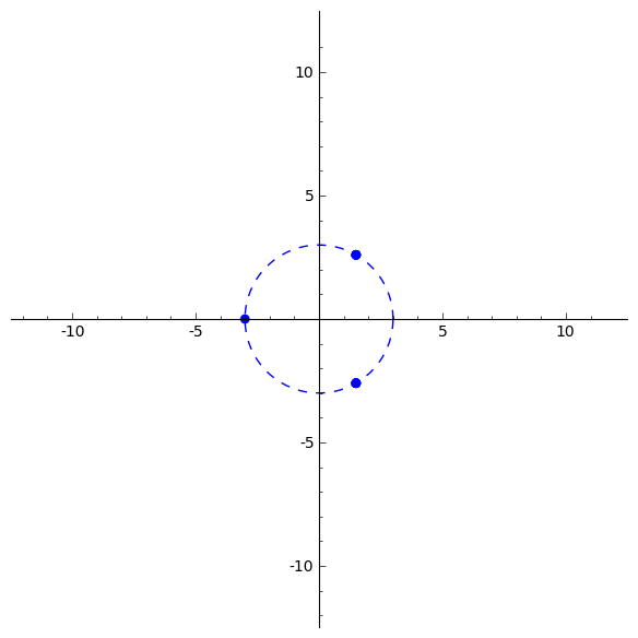
Figure 5: The plot of the values of the Hadamard transform of $f$ in the complex plane of the even $GF(3)$-valued bent function of two variables from Example 105. (The vertices are ordered as in Example 105.)

The set of such functions has some amusing combinatorial properties we shall discuss below.

There are exactly $18$ such bent functions.

$GF(3)^{2}$	(0, 0)	(1, 0)	(2, 0)	(0, 1)	(1, 1)	(2, 1)	(0, 2)	(1, 2)	(2, 2)
$b_{1}$	0	1	1	1	2	2	1	2	2
$b_{2}$	0	2	2	1	0	0	1	0	0
$b_{3}$	0	1	1	2	0	0	2	0	0
$b_{4}$	0	2	2	0	1	0	0	0	1
$b_{5}$	0	0	0	2	1	0	2	0	1
$b_{6}$	0	1	1	0	2	0	0	0	2
$b_{7}$	0	0	0	1	2	0	1	0	2
$b_{8}$	0	2	2	0	0	1	0	1	0
$b_{9}$	0	0	0	2	0	1	2	1	0
$b_{10}$	0	2	2	2	1	1	2	1	1
$b_{11}$	0	0	0	0	2	1	0	1	2
$b_{12}$	0	2	2	1	2	1	1	1	2
$b_{13}$	0	1	1	2	2	1	2	1	2
$b_{14}$	0	1	1	0	0	2	0	2	0
$b_{15}$	0	0	0	1	0	2	1	2	0
$b_{16}$	0	0	0	0	1	2	0	2	1
$b_{17}$	0	2	2	1	1	2	1	2	1
$b_{18}$	0	1	1	2	1	2	2	2	1

The unweighted Cayley graph of $b_{2}$ (as well as $b_{3}$, $b_{4}$, $b_{5}$, $b_{6}$, $b_{7}$, $b_{8}$, $b_{9}$, $b_{11}$, $b_{14}$, $b_{15}$ and $b_{16}$) is a strongly regular graph having parameters $SRG(\nu,k,\lambda,\mu)$ where $\nu=9$, $k=4$, $\lambda=1$, $\mu=2$. We say that these bent functions are of type $(9,4,1,2)$. The other $6$ bent functions are of type $(9,8,7,0)$. Up to isomorphism, there is only one (unweighted) strongly regular graph having parameters $SRG(9,4,1,2)$ [Br], [Sp]. We shall see later that the edge-weighted Cayley graphs arising from these $12$ bent functions of type $(9,4,1,2)$ are also isomorphic as weighted (strongly regular) graphs. Likewise, these $6$ bent functions of type $(9,8,7,0)$ are also isomorphic as weighted (strongly regular) graphs.

Example 106.

Let $b_{1},\dots,b_{18}$ denote the bent functions defined in §6.2. The following example shows that the dual of $b_{1}$ is $b_{10}$ and the dual of $b_{2}$ is $b_{3}$, but in one case we must pre-multiply by $-1$ and in the other case we don’t.

  Sage         sage: FF = GF(3)  sage: V = FF^2  sage: Vlist = V.list()  sage: flist = [0, 1, 1, 1, 2, 2, 1, 2, 2]  ## this is b1  sage: f = lambda x: GF(3)(flist[Vlist.index(x)])  sage: [CC(hadamard_transform(f,a)).abs() for a in V]  [3.00000000000000, 3.00000000000000, 3.00000000000000,   3.00000000000000, 3.00000000000000, 3.00000000000000,   3.00000000000000, 3.00000000000000, 3.00000000000000]  sage: L = [CC(hadamard_transform(f,a)) for a in V]; L  [-3.00000000000000 + 1.33226762955019e-15*I,   1.50000000000000 + 2.59807621135332*I,   1.50000000000000 + 2.59807621135332*I,   1.50000000000000 + 2.59807621135332*I,   1.50000000000000 - 2.59807621135331*I,   1.50000000000000 - 2.59807621135331*I,   1.50000000000000 + 2.59807621135332*I,   1.50000000000000 - 2.59807621135331*I,   1.50000000000000 - 2.59807621135331*I]  sage: [crude_CC_log(-z/3, 3) for z in L]  [0, 2, 2, 2, 1, 1, 2, 1, 1]  ## this is b10     

Note the pre-multiplication by $-1$. This bent function $f=b_{1}:GF(3)^{2}\to GF(3)$ is weakly regular, and the weakly regular dual of $b_{1}$ is $b_{10}$.

  Sage         sage: flist = [0, 2, 2, 1, 0, 0, 1, 0, 0]  ## this is b2  sage: f = lambda x: GF(3)(flist[Vlist.index(x)])  sage: L = [CC(hadamard_transform(f,a)) for a in V]; L  [3.00000000000000 + 6.66133814775094e-16*I,   -1.50000000000000 + 2.59807621135332*I,   -1.50000000000000 + 2.59807621135332*I,   -1.50000000000000 - 2.59807621135331*I,   3.00000000000000 + 6.66133814775094e-16*I,   3.00000000000000 + 6.66133814775094e-16*I,   -1.50000000000000 - 2.59807621135331*I,   3.00000000000000 + 6.66133814775094e-16*I,   3.00000000000000 + 6.66133814775094e-16*I]  sage: [crude_CC_log(z/3, 3) for z in L]  [0, 1, 1, 2, 0, 0, 2, 0, 0]  ## this is b3       

This bent function $f=b_{2}:GF(3)^{2}\to GF(3)$ is regular, and the regular dual of $b_{2}$ is $b_{3}$.

We similar computations verify the following:

• $b_{1}$ and $b_{10}$ are both weakly regular and $-1$-dual to each other,

• $b_{2}$ and $b_{3}$ are regular and dual to each other,

• $b_{4}$ and $b_{9}$ are regular and dual to each other,

• $b_{5}$ and $b_{8}$ are regular and dual to each other,

• $b_{6}$ and $b_{15}$ are regular and dual to each other,

• $b_{7}$ and $b_{14}$ are regular and dual to each other,

• $b_{11}$ and $b_{16}$ are regular and dual to each other,

• $b_{12}$, $b_{13}$, $b_{17}$ and $b_{18}$ are all weakly regular and are each $-1$-self-dual.

Relationships:

$$b_{1}=-b_{10},\ \ b_{2}=-b_{3},\ \ b_{4}=-b_{6},\ \ b_{5}=-b_{7},\ \ b_{8}=-b_{14},$$

$$b_{9}=-b_{15},\ \ b_{11}=-b_{16},\ \ b_{12}=-b_{18},\ \ b_{13}=-b_{17},$$

$$b_{1}=b_{7}+b_{14}=b_{6}+b_{15},\ \ b_{10}=b_{4}+b_{9}=b_{5}+b_{8},\ \ b_{12}=b_{2}+b_{11}=b_{7}+b_{8},$$

$$b_{13}=b_{3}+b_{11}=b_{6}+b_{9},\ \ b_{17}=b_{2}+b_{16}=b_{4}+b_{15,}\ \ b_{18}=b_{3}+b_{16}=b_{5}+b_{14}.$$

Recall from Example 106, the following are regular

$$b_{2}^{*}=b_{3},\ \ b_{4}^{*}=b_{9},\ b_{5}^{*}=b_{8},\ b_{6}^{*}=b_{15},\ \ b_{7}^{*}=b_{14},b_{11}^{*}=b_{16},\$$

whereas

$$b_{1}^{*}=-b_{10}$$

are weakly regular and $(-1)$-dual to each other (but not regular), and the others are all $(-1)$-self-dual and weakly regular (but not regular),

$$b_{12}^{*}=-b_{12},\ b_{13}^{*}=-b_{13},\ b_{17}^{*}=-b_{17},\ b_{18}^{*}=-b_{18}.$$

Supports:

$$\{1,2,3,6\}={\rm supp}(b_{2})={\rm supp}(b_{3}),\ \ \{1,2,4,8\}={\rm supp}(b_{4})={\rm supp}(b_{6}),$$

$$\{1,2,5,7\}={\rm supp}(b_{8})={\rm supp}(b_{14}),\ \ \{3,5,6,7\}={\rm supp}(b_{9})={\rm supp}(b_{15}),$$

$$\{3,4,6,8\}={\rm supp}(b_{5})={\rm supp}(b_{7}),\ \ \{4,5,7,8\}={\rm supp}(b_{11})={\rm supp}(b_{16}),$$

and

$${\rm supp}(b_{1})={\rm supp}(b_{10})={\rm supp}(b_{12})={\rm supp}(b_{13})={\rm supp}(b_{17})={\rm supp}(b_{18})$$

are all equal to $\{1,2,3,4,5,6,7,8\}$. Note that

• All these functions are weight $4$ or weight $8$.

• If you pick any two support sets of weight $4$, $S_{1}$ and $S_{2}$ say, then they satisfy either

  $$S_{1}\cap S_{2}=\emptyset\ \ \ {\rm or}\ \ \ |S_{1}\cap S_{2}|=2.$$

• The $12$ which are regular, but not $\mu$-regular for some $\mu\not=1$) can all be obtained from $f(x_{0},x_{1})=x_{0}^{2}+x_{0}x_{1}$ by linear transformations of the coordinates, i.e. $(x_{0},x_{1})\mapsto(ax_{0}+bx_{1},cx_{0}+dx_{1})$ where $ad-bc\not=0$. Each such isomorphism of $GF(3)^{2}$ induces an isomorphism of the associated edge-weighted Cayley graphs.

• Similarly, the $6$ which are weakly regular can all be obtained from $x_{0}^{2}+x_{1}^{2}$ by linear transformations of the coordinates.

In fact, if you consider the set

$$S=\{\emptyset\}\cup\{{\rm supp}(f)\ |\ f:GF(3)^{2}\to GF(3),\ f(0)=0\},$$

then $S$ forms a group under the symmetric difference operator $\Delta$. In fact, $S\cong GF(2)^{3}$.

Question 1.

To what extent is it true that if $f_{1}$, $f_{2}$ are bent functions on $GF(p)^{n}$ with $f_{1}(0)=f_{2}(0)=0$, then

$${\rm supp}(f_{1})\,\Delta\,{\rm supp}(f_{3})={\rm supp}(f_{3})$$

for some bent function $f_{3}$ satisfying $f_{3}(0)=0$?

More general version:

Question 2.

Over $GF(p)$, $p\not=2$, does the set of supports

$$\{\emptyset\}\cup\{{\rm supp}(f)\ |\ f\mbox{ is bent},f(0)=0,f\mbox{ is even}\}$$

form a group (under $\Delta$)?

This does not seem to hold in the binary case.

The following was verified with direct (computer-aided) computations.

Lemma 107.

Assume $p=3$, $n=2$.

• The edge-weighted Cayley graph of $b_{i}$ is strongly regular and not complete as a simple (unweighted) graph if and only if $b_{i}$ is regular if and only if $i\in\{2,3,4,5,6,7,8,9,11,14,15,16\}.$

• The edge-weighted Cayley graph of $b_{i}$ is strongly regular and complete as a simple (unweighted) graph if and only if $b_{i}$ is weakly regular if and only if $i\notin\{2,3,4,5,6,7,8,9,11,14,15,16\}.$

Example 108.

This example is intended to illustrate the bent function $b_{8}$ listed in the table above, and to provide more detail on Example 26.

Consider the finite field

$$GF(9)=GF(3)[x]/(x^{2}+1)=\{0,1,2,x,x+1,x+2,2x,2x+1,2x+2\}.$$

The set of non-zero quadratic residues is given by

$$D=\{1,2,x,2x\}.$$

Let $\Gamma$ be the graph whose vertices are $GF(9)$ and whose edges $e=(a,b)$ are those pairs for which $a-b\in D$.

The graph looks like the Cayley graph for $b_{8}$ in Figure 6, except

$$8\to 0,0\to 2x+2,1\to 2x+1,2\to 2x,$$

$$3\to x+2,4\to x+1,5\to x,6\to 2,7\to 1,8\to 0.$$

This is a strongly regular graph with parameters $(9,4,1,2)$. $v$ 0 1 2 3 4 5 6 7 8 $N(v,0)$ 3,4,6,8 4,5,6,7 3,5,7,8 0,2,6,7 0,1,7,8 1,2,6,8 0,1,3,5 1,2,3,4 0,2,4,5 $N(v,1)$ 5,7 3,8 4,6 1,8 2,6 0,7 2,4 0,5 1,3 $N(v,2)$ 1,2 0,2 0,1 4,5 3,5 3,4 7,8 6,8 6,7

The axioms of an edge-weighted strongly regular graph can be directly verified using this table.

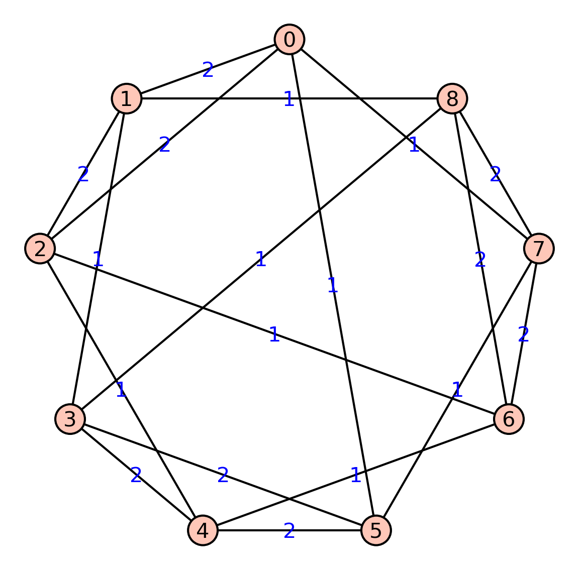
Figure 6: The Cayley graphs for $b_{8}$

6.3 Bent functions $GF(3)^{3}\to GF(3)$

Let $f:GF(3)^{3}\to GF(3)$ be an even bent function with $f(0)=0$, let

$$D_{i}=\{v\in GF(3)^{3}\ |\ f(v)=i\},\ \ \ i=1,2,$$

let $D_{0}=\{0\}$ and $D_{3}=GF(3)^{3}-(D_{0}\cup D_{1}\cup D_{2})$.

There are a total of $2340$ even bent functions on $GF(3)^{3}$.

We know that if $W_{f}(0)$ is rational then the level curves $f^{-1}(i)$, $i\not=0$, have the same cardinality. The following Sage computation shows that, in this case, $W_{f}(0)$ is not a rational number for therepresentatives of $B_{1},B_{2}$ displayed above.

  Sage         sage: PR.<x0,x1,x2> = PolynomialRing(FF, 3, "x0,x1,x2")  sage: f = x0^2 + x1^2 + x2^2  sage: V = GF(3)^3  sage: Vlist = V.list()  sage: flist = [f(x[0],x[1],x[2]) for x in Vlist]  sage: f = lambda x: FF(flist[Vlist.index(x)])  sage: hadamard_transform(f,V(0))  12*e^(4/3*I*pi) + 6*e^(2/3*I*pi) + 9  sage: CC(hadamard_transform(f,V(0)))  -3.99680288865056e-15 - 5.19615242270663*I  sage: f = x0*x2 + 2*x1^2 + 2*x0^2*x2^2  sage: flist = [f(x[0],x[1],x[2]) for x in Vlist]  sage: f = lambda x: FF(flist[Vlist.index(x)])  sage: hadamard_transform(f,V(0))  14*e^(4/3*I*pi) + 2*e^(2/3*I*pi) + 11  sage: CC(hadamard_transform(f,V(0)))  2.99999999999999 - 10.3923048454133*I     

Using Sage, we give some examples of an even bent function of $3$ variables over $GF(3)$.

  Sage         sage: FF = GF(3)  sage: V = FF^3  sage: Vlist = V.list()  sage: Vlist  [(0, 0, 0), (1, 0, 0), (2, 0, 0), (0, 1, 0), (1, 1, 0), (2, 1, 0),  (0, 2, 0), (1, 2, 0), (2, 2, 0), (0, 0, 1), (1, 0, 1), (2, 0, 1),  (0, 1, 1), (1, 1, 1), (2, 1, 1), (0, 2, 1), (1, 2, 1), (2, 2, 1),  (0, 0, 2), (1, 0, 2), (2, 0, 2), (0, 1, 2), (1, 1, 2), (2, 1, 2),  (0, 2, 2), (1, 2, 2), (2, 2, 2)]  sage: flist = [0,2,2,1,1,1,1,1,1,2,0,1,1,2,0,1,0,0,2,1,0,1,0,0,1,0,2]  sage: f = lambda x: GF(3)(flist[Vlist.index(x)])  sage: [f(a)- f(-a) for a in V]  [0, 0, 0, 0, 0, 0, 0, 0, 0, 0, 0, 0, 0, 0, 0, 0, 0, 0, 0, 0, 0, 0, 0, 0, 0, 0, 0]  sage: [CC(hadamard_transform(f,a)).abs() for a in V]  [5.19615242270663, 5.19615242270663, 5.19615242270664, 5.19615242270663,   5.19615242270663, 5.19615242270663, 5.19615242270663, 5.19615242270663,   5.19615242270663, 5.19615242270663, 5.19615242270663, 5.19615242270663,   5.19615242270663, 5.19615242270664, 5.19615242270663, 5.19615242270663,   5.19615242270663, 5.19615242270663, 5.19615242270664, 5.19615242270663,   5.19615242270663, 5.19615242270663, 5.19615242270663, 5.19615242270663,   5.19615242270663, 5.19615242270663, 5.19615242270664]  sage: supp_f = [Vlist.index(x) for x in V if f(x)<>0]; supp_f  [1, 2, 3, 4, 5, 6, 7, 8, 9, 11, 12, 13, 15, 18, 19, 21, 24, 26]     

Since $W_{f}(0)/3^{3/2}$ is a $6$-th root of unity, but not a cube root of unity, it follows from Lemma 11 that $f$ is not weakly regular.

  Sage         sage: a = 2; b = 4; c = 4  sage: flist = [0,a,a,c,b,1,c,1,b,2,0,1,1,2,0,1,0,0,2,1,0,1,0,0,1,0,2]  sage: f = lambda x: GF(3)(flist[Vlist.index(x)])  sage: [f(a)- f(-a) for a in V]  [0, 0, 0, 0, 0, 0, 0, 0, 0, 0, 0, 0, 0, 0, 0, 0, 0, 0, 0, 0, 0, 0, 0, 0, 0, 0, 0]  sage: [CC(hadamard_transform(f,a)).abs() for a in V]  [5.19615242270663, 5.19615242270663, 5.19615242270664, 5.19615242270663,   5.19615242270663, 5.19615242270663, 5.19615242270663, 5.19615242270663,   5.19615242270663, 5.19615242270663, 5.19615242270663, 5.19615242270663,   5.19615242270663, 5.19615242270664, 5.19615242270663, 5.19615242270663,   5.19615242270663, 5.19615242270663, 5.19615242270664, 5.19615242270663,   5.19615242270663, 5.19615242270663, 5.19615242270663, 5.19615242270663,   5.19615242270663, 5.19615242270663, 5.19615242270664]  sage: supp_f = [Vlist.index(x) for x in V if f(x)<>0]; supp_f  [1, 2, 3, 4, 5, 6, 7, 8, 9, 11, 12, 13, 15, 18, 19, 21, 24, 26]     

Here are some algebraic examples:

  Sage         sage: R.<x0,x1,x2> = PolynomialRing(FF,3,"x0,x1,x2")  sage: V = GF(3)^3  sage: ff = x1^2+x0*x2  sage: flist = [ff(x0=v[0],x1=v[1],x2=v[2]) for v in V]  sage: Vlist = V.list()  sage: f = lambda x: GF(3)(flist[Vlist.index(x)])  sage: [CC(hadamard_transform(f,a)).abs() for a in V]  [5.19615242270663, 5.19615242270663, 5.19615242270663,  5.19615242270663, 5.19615242270663, 5.19615242270663,  5.19615242270663, 5.19615242270663, 5.19615242270663,  5.19615242270663, 5.19615242270663, 5.19615242270663,  5.19615242270663, 5.19615242270663, 5.19615242270663,  5.19615242270663, 5.19615242270663, 5.19615242270663,  5.19615242270663, 5.19615242270663, 5.19615242270663,  5.19615242270663, 5.19615242270663, 5.19615242270663,  5.19615242270663, 5.19615242270663, 5.19615242270663]  sage:  sage: ff = x1^2+x0*x2+x1+2*x0  sage: flist = [ff(x0=v[0],x1=v[1],x2=v[2]) for v in V]  sage: f = lambda x: GF(3)(flist[Vlist.index(x)])  sage: [CC(hadamard_transform(f,a)).abs() for a in V]  [5.19615242270663, 5.19615242270663, 5.19615242270663,  5.19615242270663, 5.19615242270663, 5.19615242270663,  5.19615242270663, 5.19615242270663, 5.19615242270663,  5.19615242270663, 5.19615242270663, 5.19615242270663,  5.19615242270663, 5.19615242270663, 5.19615242270663,  5.19615242270663, 5.19615242270663, 5.19615242270663,  5.19615242270663, 5.19615242270663, 5.19615242270663,  5.19615242270663, 5.19615242270663, 5.19615242270663,  5.19615242270663, 5.19615242270663, 5.19615242270663]     

Note the first example is even but the second one is not.

6.4 Bent functions $GF(5)^{2}\to GF(5)$

Using Sage, we give examples of bent functions of $2$ variables over $GF(5)$ and study their signatures (14).

Do the “level curves” of a bent function $GF(5)^{2}\to GF(5)$ give rise to a PDS? An association scheme (see below for a definition)?

Example 109.

Let $G=GF(25)=GF(5)[x]/(x^{2}+2)$,

$$D_{1}=\{1,4,x+2,4x+3\},D_{2}=\{x+1,x+3,4x+2,4x+4\},$$

$$D_{3}=\{2x+1,2x+2,3x+3,3x+4\},D_{4}=\{2,3,2x+4,3x+1\},$$

and $D=D_{1}\cup D_{2}\cup D_{3}\cup D_{4}$. If $f(x_{0},x_{1})=x_{0}^{2}+x_{0}x_{1}$ then each subset $D_{i}$ ($i=1,2,3,4$) is the image of the level curve $f^{-1}(i)$ under the $GF(5)$-vector space isomorphism

$$\begin{array}[]{ccc}\phi\,:\,GF(5)^{2}&\to&GF(25),\\ (a,b)&\longmapsto&bx+a\,,\\ \end{array}$$

$D_{i}=\phi(f^{-1}(i))$, $i=1,2,3,4$. As in the previous example, we can compute the $k_{i,j}$’s, $\mu_{i,j}$’s, and $\lambda_{i,j}^{k}$’s (see Example 94 for the details). This $f$ is homogeneous, bent and regular (hence also weakly regular).

The weighted adjacency matrix $A$ of the edge-weighted Cayley graph associated to $f$, $\Gamma_{f}$, is given below:

$$\left(\begin{array}[]{rrrrrrrrrrrrrrrrrrrrrrrrr}0&1&4&4&1&0&2&1&2&0&0&3&3&0&4&0&4&0&3&3&0&0&2&1&2\\ 1&0&1&4&4&0&0&2&1&2&4&0&3&3&0&3&0&4&0&3&2&0&0&2&1\\ 4&1&0&1&4&2&0&0&2&1&0&4&0&3&3&3&3&0&4&0&1&2&0&0&2\\ 4&4&1&0&1&1&2&0&0&2&3&0&4&0&3&0&3&3&0&4&2&1&2&0&0\\ 1&4&4&1&0&2&1&2&0&0&3&3&0&4&0&4&0&3&3&0&0&2&1&2&0\\ 0&0&2&1&2&0&1&4&4&1&0&2&1&2&0&0&3&3&0&4&0&4&0&3&3\\ 2&0&0&2&1&1&0&1&4&4&0&0&2&1&2&4&0&3&3&0&3&0&4&0&3\\ 1&2&0&0&2&4&1&0&1&4&2&0&0&2&1&0&4&0&3&3&3&3&0&4&0\\ 2&1&2&0&0&4&4&1&0&1&1&2&0&0&2&3&0&4&0&3&0&3&3&0&4\\ 0&2&1&2&0&1&4&4&1&0&2&1&2&0&0&3&3&0&4&0&4&0&3&3&0\\ 0&4&0&3&3&0&0&2&1&2&0&1&4&4&1&0&2&1&2&0&0&3&3&0&4\\ 3&0&4&0&3&2&0&0&2&1&1&0&1&4&4&0&0&2&1&2&4&0&3&3&0\\ 3&3&0&4&0&1&2&0&0&2&4&1&0&1&4&2&0&0&2&1&0&4&0&3&3\\ 0&3&3&0&4&2&1&2&0&0&4&4&1&0&1&1&2&0&0&2&3&0&4&0&3\\ 4&0&3&3&0&0&2&1&2&0&1&4&4&1&0&2&1&2&0&0&3&3&0&4&0\\ 0&3&3&0&4&0&4&0&3&3&0&0&2&1&2&0&1&4&4&1&0&2&1&2&0\\ 4&0&3&3&0&3&0&4&0&3&2&0&0&2&1&1&0&1&4&4&0&0&2&1&2\\ 0&4&0&3&3&3&3&0&4&0&1&2&0&0&2&4&1&0&1&4&2&0&0&2&1\\ 3&0&4&0&3&0&3&3&0&4&2&1&2&0&0&4&4&1&0&1&1&2&0&0&2\\ 3&3&0&4&0&4&0&3&3&0&0&2&1&2&0&1&4&4&1&0&2&1&2&0&0\\ 0&2&1&2&0&0&3&3&0&4&0&4&0&3&3&0&0&2&1&2&0&1&4&4&1\\ 0&0&2&1&2&4&0&3&3&0&3&0&4&0&3&2&0&0&2&1&1&0&1&4&4\\ 2&0&0&2&1&0&4&0&3&3&3&3&0&4&0&1&2&0&0&2&4&1&0&1&4\\ 1&2&0&0&2&3&0&4&0&3&0&3&3&0&4&2&1&2&0&0&4&4&1&0&1\\ 2&1&2&0&0&3&3&0&4&0&4&0&3&3&0&0&2&1&2&0&1&4&4&1&0\end{array}\right)$$

This is verified using the following Sage commands:

  Sage         sage: attach "/home/wdj/sagefiles/hadamard_transform.sage"  sage: FF = GF(5)  sage: V = FF^2  sage: R.<x0,x1> = PolynomialRing(FF,2,"x0,x1")  sage: ff = x0^2+x0*x1  sage: flist = [ff(x0=v[0],x1=v[1]) for v in V]  sage: Vlist = V.list()  sage: f = lambda x: FF(flist[Vlist.index(x)])  sage: Gamma = boolean_cayley_graph(f, V)  sage: A = Gamma.weighted_adjacency_matrix(); A  25 x 25 sparse matrix over Finite Field of size 5       

First, we consider the bent regular function $f(x_{0},x_{1})=x_{0}^{2}+x_{0}x_{1}$.

  Sage         sage: FF = GF(5)  sage: V = FF^2  sage: R.<x0,x1> = PolynomialRing(FF,2,"x0,x1")  sage: ff = x0^2+x0*x1  sage: flist = [ff(x0=v[0],x1=v[1]) for v in V]  sage: Vlist = V.list()  sage: f = lambda x: FF(flist[Vlist.index(x)])  sage: [CC(hadamard_transform(f,a)).abs() for a in V]  [5.00000000000000, 5.00000000000000, 5.00000000000000,  5.00000000000000, 5.00000000000000, 5.00000000000000,  5.00000000000000, 5.00000000000000, 5.00000000000000,  5.00000000000000, 5.00000000000000, 5.00000000000000,  5.00000000000000, 5.00000000000000, 5.00000000000000,  5.00000000000000, 5.00000000000000, 5.00000000000000,  5.00000000000000, 5.00000000000000, 5.00000000000000,  5.00000000000000, 5.00000000000000, 5.00000000000000,  5.00000000000000]  sage: Gamma = boolean_cayley_graph(f, V)  sage: Gamma.connected_components_number()  1  sage: Gamma.spectrum()  [16, 1, 1, 1, 1, 1, 1, 1, 1, 1, 1, 1, 1, 1, 1, 1, 1, -4, -4, -4, -4,  -4, -4, -4, -4]       

Next, we consider $f(x_{0},x_{1})=x_{0}^{2}+x_{1}^{2}$, having signature $[9,4,4,4,4]$. This is also regular bent.

  Sage         sage: ff = x0^2+x1^2  sage: flist = [FF(x) for x in flist]  sage: f = lambda x: FF(flist[Vlist.index(x)])  sage: ff = x0^2+x1^2  sage: flist = [ff(x0=v[0],x1=v[1]) for v in V]  sage: f = lambda x: FF(flist[Vlist.index(x)])  sage: flist = [FF(x) for x in flist]  sage: [CC(hadamard_transform(f,a)).abs() for a in V]  [5.00000000000000, 5.00000000000000, 5.00000000000000,   5.00000000000000, 5.00000000000000, 5.00000000000000,   5.00000000000000, 5.00000000000000, 5.00000000000000,   5.00000000000000, 5.00000000000000, 5.00000000000000,   5.00000000000000, 5.00000000000000, 5.00000000000000,   5.00000000000000, 5.00000000000000, 5.00000000000000,   5.00000000000000, 5.00000000000000, 5.00000000000000,   5.00000000000000, 5.00000000000000, 5.00000000000000,   5.00000000000000]  sage: flist  [0, 1, 4, 4, 1, 1, 2, 0, 0, 2, 4, 0, 3, 3, 0, 4, 0, 3, 3, 0, 1, 2, 0, 0, 2]  sage: fcount = [flist.count(x) for x in FF]; fcount  [9, 4, 4, 4, 4]       

Not that this is even and the signature agrees with Lemma 56.

Finally, we consider $f(x_{0},x_{1})=x_{0}^{2}+2x_{1}^{2}+x_{0}$, having signature $[4,9,4,4,4]$. This is also regular bent.

  Sage         sage: ff = x0^2-x1^2+x0  sage: flist = [ff(x0=v[0],x1=v[1]) for v in V]  sage: f = lambda x: FF(flist[Vlist.index(x)])  sage: [CC(hadamard_transform(f,a)).abs() for a in V]  [5.00000000000000, 5.00000000000000, 5.00000000000000,   5.00000000000000, 5.00000000000000, 5.00000000000000,   5.00000000000000, 5.00000000000000, 5.00000000000000,   5.00000000000000, 5.00000000000000, 5.00000000000000,   5.00000000000000, 5.00000000000000, 5.00000000000000,   5.00000000000000, 5.00000000000000, 5.00000000000000,   5.00000000000000, 5.00000000000000, 5.00000000000000,   5.00000000000000, 5.00000000000000, 5.00000000000000,   5.00000000000000]  sage: flist = [FF(x) for x in flist]; flist  [0, 2, 1, 2, 0, 4, 1, 0, 1, 4, 1, 3, 2, 3, 1, 1, 3, 2, 3, 1, 4, 1, 0, 1, 4]  sage: fcount = [flist.count(x) for x in FF]; fcount  [4, 9, 4, 4, 4]       

Example 110.

Consider the bent function

$$f_{4}(x_{0},x_{1})=-x_{1}^{4}-2x_{1}^{2}+x_{0}x_{1}.$$

This function represents a $GL(2,GF(5))$ orbit of size $120$. The level curves of this function do not give rise to a weighted PDS. By the way, if we try a computation of all the $p_{ij}^{k}$’s as in the above example, we do not get integers.

Similarly, the level curves of $f_{7}$, $f_{8}$, $f_{10}$, and $f_{11}$ do not give rise to a weighted PDS.

Example 111.

The example of $f_{5}$ above can be used to construct an edge-weighted strongly regular Cayley graph, hence also a weighted PDS attached to its level curves. The examples of $f_{6}$ and $f_{9}$ above have an isomorphic weighted PDS attached to their (respective) level curves.

Acknowledgements: We are grateful to our colleague T. S. Michael for many stimulating conversations and suggestions on this paper.

7 Appendix: A new search algorithm for bent functions

The following algorithm and code is due to the first author C. Celerier.

  Python        from collections import defaultdict  from copy import deepcopy  from random import shuffle  from sage.crypto.boolean_function import BooleanFunction    class NoBentFunction(Exception):      pass    class BentFinder(object):      def __init__(self, n):          self.V = GF(2)**n          self.n = n        def searchForBent(self):          self.walshTrace = []          A = defaultdict(int)          W = defaultdict(int)          B = list(self.V.list())          shuffle(B)          R = self.__searchForBent(A,B,W,0)          self.walshTrace.reverse()          return BooleanFunction([R[tuple(x)] for x in self.V]), self.walshTrace        def __searchForBent(self, A, B, W, wgt):          n = self.n          if len(A) == 2**n:              return A          if wgt > 2**(n-1)-2**(n/2-1):              raise NoBentFunction            A,B,W,wgt = self.__deepcopy(A,B,W,wgt)          v = B.pop()          cf = self.__coinFlip()          values = (cf, (1+cf) % 2)          for a in values:              try:                  A[tuple(v)] = a                  update = self.__getUpdate(v, a)                  W_a = self.__applyUpdate(W, update, 2**n-len(A))                  R = self.__searchForBent(A,B,W_a,wgt+a)                  self.walshTrace.append((v, A[tuple(v)], [W_a[x] for x in W_a]))                  return R              except NoBentFunction:                  pass          raise NoBentFunction        def __applyUpdate(self, W, update, leftToFill):          n = self.n          W = deepcopy(W)          for u in self.V:              W[tuple(u)] += update[tuple(u)]              Wmin = W[tuple(u)] - leftToFill              Wmax = W[tuple(u)] + leftToFill              if not ((Wmin <= 2**(n/2) and 2**(n/2) <= Wmax) or (Wmin <= -2**(n/2) and -2**(n/2) <= Wmax)):                  raise NoBentFunction          return W        def __getUpdate(self,v,a):          update = {}          for u in self.V:              update[tuple(u)] = Integer(-1)**(a+u.dot_product(v))          return update        def __deepcopy(self, *args):          R = []          for a in args:              R.append(deepcopy(a))          return R        def __coinFlip(self):          return 1 if random() > .5 else 0       

An example:

  Sage         sage: %attach bentFunctions.sage  sage: B=BentFinder(4)  sage: B.searchForBent()  (Boolean function with 4 variables,   [((0, 0, 0, 1), 1, [1, 1, 1, 1, 1, 1, 1, 1, 1, 1, 1, 1, 1, 1, 1, 1]),    ((0, 1, 0, 0), 0, [2, 2, 0, 0, 0, 0, 2, 2, 2, 0, 2, 0, 0, 2, 0, 2]),    ((1, 1, 0, 1), 1, [1, 3, 1, 1, -1, -1, 3, 3, 3, 1, 1, 1, -1, 1, -1, 1]),    ((0, 1, 1, 1), 0, [2, 2, 2, 2, 0, -2, 4, 4, 2, 0, 2, 0, 0, 0, -2, 0]),    ((0, 0, 1, 0), 1, [3, 3, 1, 3, 1, -3, 3, 5, 1, -1, 1, 1, -1, 1, -1, -1]),    ((0, 0, 1, 1), 0, [2, 4, 2, 2, 0, -4, 2, 6, 0, 0, 2, 2, -2, 0, 0, 0]),    ((0, 1, 0, 1), 0, [1, 5, -1, 3, 1, -3, 1, 7, -1, -1, 3, 1, -1, 1, -1, 1]),    ((0, 1, 1, 0), 0, [2, 4, 4, 2, 2, -4, 0, 6, -2, 0, 4, 0, -2, 0, -2, 2]),    ((1, 1, 0, 0), 1, [1, 3, -1, 5, 1, -5, 1, 5, -1, -1, 5, 3, -3, 1, -1, 3]),    ((1, 0, 1, 1), 0, [0, 4, 6, 2, 2, -6, 0, 4, 0, -2, 4, 2, -2, 0, -2, 4]),    ((1, 0, 0, 0), 1, [1, 3, -1, 5, 1, -7, -1, 5, 1, -3, 3, 3, -1, 3, -1, 5]),    ((1, 1, 1, 0), 0, [2, 4, 6, 4, 2, -6, -2, 4, 2, -4, 4, 0, -2, -2, 0, 4]),    ((1, 0, 0, 1), 0, [3, 5, -3, 5, 1, -5, -1, 3, 1, -5, 3, 3, -3, 5, -1, 5]),    ((1, 1, 1, 1), 0, [4, 6, 4, 4, 4, -6, -2, 2, 2, -4, 4, 2, -2, -4, -2, 4]),    ((1, 0, 1, 0), 1, [3, 5, -3, 3, 3, -5, -3, 3, 3, -5, 5, 5, -3, 5, -3, 3]),    ((1, 0, 1, 0), 1, [4, 4, 4, 4, 4, -4, -4, 4, 4, -4, 4, 4, -4, -4, -4, 4])])

References

- [BD] John J. Benedetto and Somantika Datta, Constructions and a generalization of perfect autocorrelation sequences on , preprint.
- [B] Anna Bernasconi, Mathematical techniques for the analysis of Boolean functions, Ph. D. dissertation TD-2/98, Universit di Pisa-Udine, 1998.
-
[BC]
Anna Bernasconi and Bruno Codenotti, Spectral analysis
of Boolean functions as a graph eigenvalue problem,
IEEE Transactions on Computers, 48:3 (1999) 345-351.
http://ilex.iit.cnr.it/codenotti/ps_files/graph_fourier.ps - [BCV] A. Bernasconi, B. Codenotti, J.M. VanderKam. A characterization of bent functions in terms of strongly regular graphs, IEEE Transactions on Computers, 50:9 (2001), 984-985.
- [Br] A. Brouwer, webpage Parameters of Strongly Regular Graphs at http://www.win.tue.nl/~aeb/graphs/srg/srgtab1-50.html
- [BrCN] A. Brouwer, A. Cohen, A. Neumaier, Distance-Regular Graphs, New York: Springer-Verlag, 1989.
- [CvL] P. Cameron and J. van Lint, Designs, Graphs, Codes and Their Links, London Math. Soc. Lecture Note Series, Vol. 19, Cambridge University Press, 1991.
-
[C]
C. Carlet, Boolean functions for cryptography and error
correcting codes,
in Boolean Models and Methods in Mathematics, Computer Science,
and Engineering,
Cambridge University Press, edited by Yves Crama and Peter L. Hammer,
pp. 257-397, 2010.
http://www1.spms.ntu.edu.sg/~kkhoongm/chap-fcts-Bool.pdf - [CD] —–, C. Ding, Highly non-linear mappings, J. of Complexity, 20(2004)205-244.
-
[CJMP]
C. Celerier, D. Joyner, C. Melles, D. Phillips,
On the Walsh-Hadamard transform of monotone Boolean functions,
Tbilisi Mathematical Journal
(Special Issue on Sage and Research)
5(2012)19-35.
http://www.wdjoyner.org/papers/monotone-boolean-fcns-tmj2012-06-20.pdf - [CM] A. Cesmelioglu and W. Meidl, Bent functions of maximal degree, IEEE Trans. Info. Theory 58(2012)1186-1190.
-
[CTZ]
Y. Chee, Y. Tan, X. Zhang, Strongly regular graphs constructed
from -ary bent functions, preprint, 2010.
http://arxiv.org/abs/1011.4434. - [CP] Yu Qing Chen, John Polhill, Partial difference sets and amorphic group schemes from pseudo-quadratic bent functions, J Algebr Comb 37(2013)11-26.
- [CoM] Robert Coulter and Rex Matthews, Bent polynomials over finite fields, Bull. Austral. Math. Soc. 56(1977)429-437.
- [De] P. Delsarte, An algebraic approach to the association schemes of coding theory, Philips Res. Rep. Suppl. No. 10 (1973).
- [D] J.F. Dillon, Elementary Hadamard Difference Sets, PhD thesis, University of Maryland, 1974.
- [FWXY] T. Fen, B. Wen, Q. Xiang, J. Yin, Partial difference sets from quadratic forms and -ary weakly regular bent functions, Number Theory and Related Areas, ALM 27(2010)25-40.
- [F] Miroslav Fiedler. Algebraic connectivity of graphs. Czechoslovak Math. Journal. 23(98):298–305, 1973.
- [HK] Tor Helleseth and Alexander Kholosha, On Generalized Bent Functions, Information theory and applications workshop(ITA), 2010.
- [HK2] —— and ——, Connections between bent functions and combinatorics, in Surveys in Combinatorics 2013 (London Mathematical Society Lecture Note Series) Cambridge University Press, 2013.
- [HK3] —— and ——, Monomial and Quadratic Bent Functions over the Finite Fields of Odd Characteristic, IEEE Trans. Info. Theory 52 (2006)2018 - 2032.
-
[He]
A. Herman,
Seminar Notes: Algebraic Aspects of Association Schemes and Scheme Rings,
seminar notes, 2011.
http://uregina.ca/~hermana/ASSR-Lecture9.pdf - [H] X.-D. Hou, p-Ary and q-ary versions of certain results about bent functions and resilient functions, Finite Fields and it Appl. 10(2004)566-582.
- [KSW] P.V Kumar, R.A Scholtz, L.R Welch, Generalized bent functions and their properties, Journal of Combinatorial Theory, Series A, Volume 40, Issue 1, September 1985, Pages 90–107.
-
[Po]
J. Polhill, A brief survey of difference sets,
partial difference sets, and relative difference sets, preprint, 2003.
http://www.passhema.org/proceedings/2003/PolhillDifference2003.pdf - [PTFL] A. Pott, Y. Tan, T. Feng, S. Ling, Association schemes arising from bent functions, Des. Codes Crypt. 59(2011)319-331.
- [Sp] E. Spence, webpage Strongly Regular Graphs on at most 64 vertices at http://www.maths.gla.ac.uk/~es/srgraphs.php
- [St] Pantelimon Stanica, Graph eigenvalues and Walsh spectrum of Boolean functions, INTEGERS 7(2) (2007), #A32.
-
[T]
N. Tokareva, Generalizations of bent functions: a
survey, 2010.
http://eprint.iacr.org/2011/111.pdf - [vD] E. van Dam, Strongly regular decompositions of complete graphs, preprint 2001.
Index
- adjacency matrix §2.1
- adjacency ring §2.2
- association scheme §2.2
- balanced §3
- bent §1
-