Long range dependence and the dynamics of exploited fish populations

Abstract

Long range dependence or long memory is a feature of many processes in the natural world, which provides important insights on the underlying mechanisms that generate the observed data. The usual tools available to characterize the phenomenon are mostly based on second order correlations. However, the long memory effects may not be evident at the level of second order correlations and may require a deeper analysis of the nature of the stochastic processes.

After a short review of the notions and tools used to characterize long range dependence, we analyse data related to the abundance of exploited fish populations which provides an example of higher order long range dependence.

1 Introduction

Long range dependence or long memory is an important notion in many processes in the natural world. Studies involving this notion pervade fields from biology to econometrics, linguistics, hydrology, climate, DNA sequencing, etc. Although, at times, it has been considered a nuisance in the study of these processes, the existence of long memory is in fact a bonus, in the sense that it provides further insight in the nature of the process. Whereas short or no memory just points out to the essentially unstructured nature of the phenomena, long memory, by contrast, may provide a window on the underlying mechanisms that generate the observed data.

The most popular definitions of long range dependence are based on the second-order properties of the processes and relate to the asymptotic behavior of covariances, spectral densities and variances of partial sums. However there are other different points of view, some of which are not equivalent to the characterization of second-order properties. They include ergodic theory notions, limiting behavior, large deviations, fractional differentiation, etc. [1] [2] [3].

When looking for or extracting long range dependence from a time series, two important warnings should be taken into account. First, long range dependence may be mimicked by lack of stationarity or by a change of regime. Long range dependence is a notion that refers to stationary processes. Second, long range dependence is a feature which may only be associated to the higher order characteristics of the process. A process that looks short range when looked at through second-order properties, may in fact have an underlying long range dependence of higher order properties.

In Section 2 we collect a few definitions of the most usual parameters, used to characterize long range dependence, that will be useful later on and in Section 3 analyze some data related to the abundance of exploited fish populations which provides an example of higher order long range dependence.

2 Notions and tools for long-range dependence

When based on second order properties, long range dependence in a stationary time series $X\left(t\right)$ occurs when the covariances

$$\gamma\left(\tau\right)=\mathbb{E}\left\{X\left(t\right)X\left(t+\tau\right)\right\}$$ (1)

tend to zero so slowly that their sum

$$\sum_{\tau=0}^{\infty}\gamma\left(\tau\right)$$ (2)

diverges. Alternative definitions of long-range dependence are based on the power-law behavior of the covariances, namely

$$\begin{array}[]{cccccc}\sum_{\tau=-n}^{n}\gamma\left(\tau\right)&\backsim&n^{\alpha}L_{1}\left(n\right)&\text{when}&n\rightarrow\infty&;0<\alpha<1\\ \gamma\left(\tau\right)&\backsim&\tau^{-\beta}L_{2}\left(\tau\right)&\text{when}&\tau\rightarrow\infty&;0<\beta<1\\ f\left(\nu\right)&\backsim&\left|\nu\right|^{-\xi}L_{3}\left(\left|\nu\right|\right)&\text{when}&\nu\rightarrow 0&;0<\xi<1\end{array}$$ (3)

$f\left(\nu\right)$ being the spectral density

$$f\left(\nu\right)=\frac{1}{2\pi}\sum_{\tau=-\infty}^{\infty}e^{-i\nu\tau}\gamma\left(\tau\right)$$ (4)

$L_{1},L_{2}$ being slowly varying functions at infinity and $L_{3}$ slowly varying at zero.

If $\gamma\left(\tau\right)$ is monotone as $\tau\rightarrow\infty$, the definitions (3) are equivalent to the divergence of the sum in (2) with $\alpha=1-\beta$ and $\xi=1-\beta$.

In science, one of the main purposes when observing natural phenomena is the construction of models. A useful approach in this endeavour is the comparison of natural time series with the behavior of well-studied mathematical structures. In the context of long range dependence a central role is played by the theory of self-similar stochastic processes

$$X\left(at\right)\overset{d}{=}a^{H}X\left(t\right)$$ (5)

with stationary increments

$$X\left(t+h\right)-X\left(t\right)\overset{d}{=}X\left(t\right)-X\left(0\right)$$ (6)

$\overset{d}{=}$ meaning equality in distribution. These processes are denoted as $H-sssi$ processes and $H$ is called the Hurst exponent. Notice that there is a close relation between self-similarity and stationarity. If $X\left(t\right)$ is self-similar then $Y\left(t\right)=e^{-tH}X\left(t\right)$ is stationary and conversely if $Y\left(t\right)$ is stationary $X\left(t\right)=t^{H}Y\left(\ln t\right)$ is self-similar.

A finite $\sigma^{2}$ variance $H-sssi$ process has a covariance

$$\mathbb{E}\left\{X\left(s\right)X\left(t\right)\right\}=\frac{\sigma^{2}}{2}\left\{\left|t\right|^{2H}+\left|s\right|^{2H}-\left|t-s\right|^{2H}\right\}$$ (7)

Throughout this paper $\mathbb{E}\left\{\cdots\right\}$ will denote the expected value which, for all the data examples, one approximates by the empirical average $\left\langle\cdots\right\rangle$.

There are non-Gaussian $H-sssi$ processes as well as $H-sssi$ processes with infinite covariance [4]. However, the simplest example of a $H-sssi$ process is a Gaussian process uniquely defined by the covariance (7) and normalized to have $\sigma^{2}=1$. It is called fractional Brownian motion (fBm) $B_{H}\left(t\right)$ and the increment process

$$Z\left(t\right)=B_{H}\left(t+1\right)-B_{H}\left(t\right)$$ (8)

is called fractional Gaussian noise (fGn). For $H=\frac{1}{2}$, $B_{1/2}\left(t\right)$ is Brownian motion. Fractional Gaussian noise has covariance

$$\gamma\left(\tau\right)=\frac{1}{2}\left\{\left|\tau+1\right|^{2H}-2\left|\tau\right|^{2H}+\left|\tau-1\right|^{2H}\right\}$$ (9)

hence, if $H=\frac{1}{2}$ it has $\gamma\left(\tau\right)=0$ (no memory) and for $H\neq\frac{1}{2}$ and large $\tau$

$$\gamma\left(\tau\right)\backsim H\left(2H-1\right)\left|\tau\right|^{2H-2}\hskip 42.67912pt\tau\rightarrow\infty$$ (10)

For $\frac{1}{2}<H<1$ the process has long range dependence. Because $\gamma\left(\tau\right)>0$ for $H>\frac{1}{2}$ and $\gamma\left(\tau\right)<0$ for $H<\frac{1}{2}$, the process is called persistent in the first case and anti-persistent in the second. For the spectral function at $H\neq\frac{1}{2}$

$$f\left(\nu\right)\backsim\nu^{1-2H}\hskip 42.67912pt\nu\rightarrow 0$$ (11)

which for $H>\frac{1}{2}$ blows up at the origin.

The Hurst exponent ($H$) as an index of long range dependence quantifies the tendency of a time series either to regress strongly to the mean or to persist in a deviation from the mean. An $H$ value between $0.5$ and $1$ signals a time series with long-term positive autocorrelation, meaning that a high (or low) value in the series will probably be followed by another high (or low) value. A value in the range $0$ to $0.5$ signals long-term switching between high and low values, meaning that an high value will probably be followed by a low value, with this tendency to switch between high and low values lasting into the future.

Although the correlation behavior of the fractional processes is very different from simple Brownian motion, they may be represented as integrals of Brownian motion with the appropriate integration kernel. For example

$$B_{H}\left(t\right) = \int_{-\infty}^{0}\left\{\left(t-u\right)^{H-\frac{1}{2}}-\left(-u\right)^{H-\frac{1}{2}}\right\}dB\left(u\right)$$ (12)

$$+\int_{0}^{t}\left(t-u\right)^{H-\frac{1}{2}}dB\left(u\right)$$

where $B\left(u\right)=B_{\frac{1}{2}}\left(u\right)$. One practical implication is that to extract an eventual fractional behavior from the data it is not sufficient an observation of short time intervals where the process may easily be confused with an uncorrelated process.

Another way in which Brownian motion intervenes in modelling processes which are neither uncorrelated nor simple Brownian motion is through the following fundamental result of stochastic analysis [5]: If $X\left(t\right)$ is a random variable that is square-integrable in the measure generated by Brownian motion, then

$$dX\left(t\right)=\mu\left(t\right)dt+\sigma\left(t\right)dB\left(t\right)$$ (13)

where $\mu\left(t\right)$ and $\sigma\left(t\right)$ are well defined stochastic processes. Therefore although the increments of $X\left(t\right)$ have a representation in terms of the increments of Brownian motion, the process may be very different, depending on the nature of the processes $\mu\left(t\right)$ and $\sigma\left(t\right)$.

Whenever long range dependence is modelled by fractional Gaussian noise one benefits from the extensive theoretical and computational framework that is available for this process. However, fractional Gaussian noise is quite rigid in the sense that it specifies the correlations at all time lags, not only at $\tau\rightarrow\infty$. It may therefore not be suitable for modeling long range dependent phenomena where the covariance at short time lags differs from fGn. This motivated the development of other models through Gaussian linear sequences

$$X\left(t\right)=\sum_{j=-\infty}^{\infty}c_{t-j}\epsilon_{j}$$ (14)

where $\sum_{j=-\infty}^{\infty}c_{j}^{2}<\infty$ and $\left\{\epsilon_{j}\right\}_{j\in\mathbb{Z}}$ are independent identically distributed (i.i.d.) normal random variables, called innovations. A Gaussian linear sequence is stationary and for the convergence of the sum in (14) one requires

- If $\epsilon_{j}=N\left(\mu,\sigma^{2}\right)$ with $\mu\neq 0$, $\sum_{j}\left|c_{j}\right|<\infty$

- If $\epsilon_{j}=N\left(\mu,\sigma^{2}\right)$ with $\mu=0$, $\sum_{j}\left|c_{j}\right|^{2}<\infty$

An example is the FARIMA(p,d,q) process (fractional autoregressive integrated moving average) [6] [7]

$$X\left(t\right)=\Phi_{p}^{-1}\left(S\right)\Theta_{q}\left(S\right)\Delta^{-d}\epsilon_{t}\hskip 42.67912ptt\in\mathbb{Z}$$ (15)

$\left\{\epsilon_{t}\right\}$ is an i.i.d. $N\left(0,\sigma^{2}\right)$ sequence and $\Phi_{p}\left(S\right),\Theta_{q}\left(S\right)$ are polynomials on the shift operator

$$S\epsilon_{i}=\epsilon_{i-1}$$ (16)

$\Delta^{-d}$ being

$$\Delta^{-d}=\left(\mathbf{1-S}\right)^{-d}=\sum_{i=0}^{\infty}\frac{\Gamma\left(i+d\right)}{\Gamma\left(d\right)\Gamma\left(i+1\right)}S^{i}$$ (17)

The fractional differencing $\Delta^{-d}$ for $0<d<\frac{1}{2}$ models long range dependence, whereas the auto regressive $\Phi_{p}\left(S\right)$ and the moving average $\Theta_{q}\left(S\right)$ polynomials provide flexibility in modeling the short-range dependence.

Finally, as mentioned on the introduction, there are other ways to deal with long range dependence for which the behavior of covariances does not play the main role. A potentially promising way is based on ergodic theory because the notion of memory is related to the connection between a process and its shifts. Then, a possible definition of long range dependent process would be one that is ergodic but non-mixing. However the mixing property is probably not sufficiently strong to imply that a mixing stationary process has short memory. Stronger requirements may be needed. These notions will not be used here and we refer to [1] [8] for a discussion.

3 The dynamics of exploited fish populations

Long range dependence has been rarely documented in marine ecology, presumably because of the scarcity of long time series. This lack of extended time series has limited research on long memory in fish stock sizes, whose fluctuations are more often attributed to human exploitation, because most studies focus on highly exploited populations (such as the North Atlantic stocks) and over relatively short time periods. However, for a few fish populations, studies on long-term fluctuations have found long ranging trends related to human activity, mostly through overexploitation and pollution of spawning and nursery areas, environmental changes that affect the recruitment period inducing natural fluctuations in stock size and biotic processes, such as predation, cannibalism and competition [9] [10] [11].

A few years ago Niwa [12] studying the time series of 27 commercial fish stocks in the North Atlantic concluded that the variability in the population growth (the annual changes in the logarithm of population abundance $S\left(t\right)$)

$$r\left(t\right)=\ln\left(\frac{S\left(t+1\right)}{S\left(t\right)}\right)$$ (18)

is described by a Gaussian distribution. That is, the population variability process would be a geometric random walk

$$r\left(t\right)=\frac{dS\left(t\right)}{S\left(t\right)}=\sigma_{r}dB\left(t\right)$$ (19)

for some constant $\sigma_{r}$ depending on the species. The independence of the increments of Brownian motion would then imply that $r\left(t\right)$ is a purely random process.

If completely accurate this would be a sobering conclusion. Natural processes that look purely random, are processes that depend on some many uncontrollable variables that any attempt to handle them is outside our reach. This would be a serious blow to, for example, the implementation of sustentability measures.

In this paper we reanalyze some of the same type of data to confirm or sharpen the conclusions in [12]. To explore the variability in fish population growth we extracted information on the Spawning-stock biomass (SSB) data on commercial fish stocks in the North Atlantic. The available SSB time-series data are derived from age-based analytical assessments estimated by the 2013 working groups of the International Council for the Exploration of the Sea (ICES), based on the compilation of relevant data from sampling of fisheries (e.g. commercial catch-at-age) and from scientific research surveys. From the collection of available assessment data we selected three North Atlantic stocks for which the annual time-series of SSB covers at least 60 years, namely Northeast Arctic cod (Gadus morhua), Arctic haddock (Melanogrammus aeglefinus) and the North Sea autumn-spawning herring (Clupea harengus). At present, ICES classifies these stocks as having above average biomass levels with full reproductive capacity and being harvested sustainably under active management plans. The stock assessment detailed information is available at the ICES webpage [13].

For these three species we analyze the autocorrelation functions for $r\left(t\right)$ and $\left|r\left(t\right)\right|$

$$C\left(r,\tau\right)=\frac{\mathbb{E}\left\{r\left(t\right)r\left(t+\tau\right)\right\}}{\sigma^{2}}$$ (20)

$$C\left(\left|r\right|,\tau\right)=\frac{\mathbb{E}\left\{\left|r\left(t\right)\right|\left|r\left(t+\tau\right)\right|\right\}}{\sigma^{2}}$$ (21)

The results are shown in the Fig.1

Figure 1: Autocorrelation functions for $r\left(t\right)$ (upper plot) and $\left|r\left(t\right)\right|$ (lower plot)

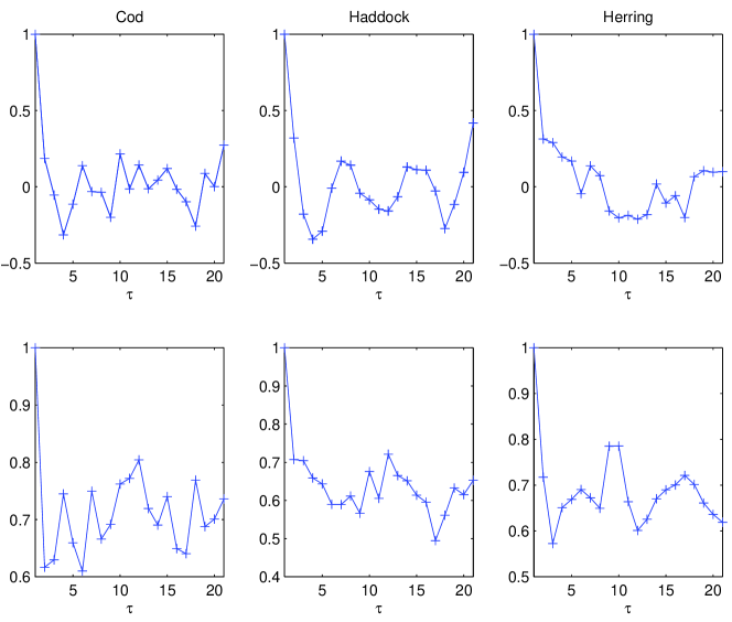
One sees that, already for time lags of one year, autocorrelations are at noise level, suggestive of uncorrelated processes. However, if $S\left(t\right)$ is indeed a geometrical Brownian motion, to rely on correlations or fitting of probability distribution functions is not sufficient. The scaling properties of $r\left(t\right)$ should be checked. As Niwa [12] rightly points out, defining

$$r_{\Delta}\left(t\right)=\ln\left\{\frac{S\left(t+\Delta\right)}{S\left(t\right)}\right\}=\sum_{i=1}^{\Delta}r\left(t+i\right)$$ (22)

the geometrical Brownian motion hypothesis would imply

$$\left(\mathbb{E}\left\{r_{\Delta}^{2}\right\}\right)^{1/2}\backsim\Delta^{1/2}$$ (23)

Normalizing $\mathbb{E}\left\{r_{\Delta}^{2}\right\}$ by the covariance $\sigma_{r}^{2}$ for each species and taking the average over all species, Niwa has obtained a behavior roughly consistent with (23). However, when we analyzed each species separately, the hypothesis does not hold. In Fig.2 we have plotted in loglog scale the computed $\left(\mathbb{E}\left\{r_{\Delta}^{2}\right\}\right)^{1/2}$ as a function of $\Delta$ for the three species analyzed in this paper.

Figure 2: $\left(\mathbb{E}\left\{r_{\Delta}^{2}\right\}\right)^{1/2}$ as a function of $\Delta$

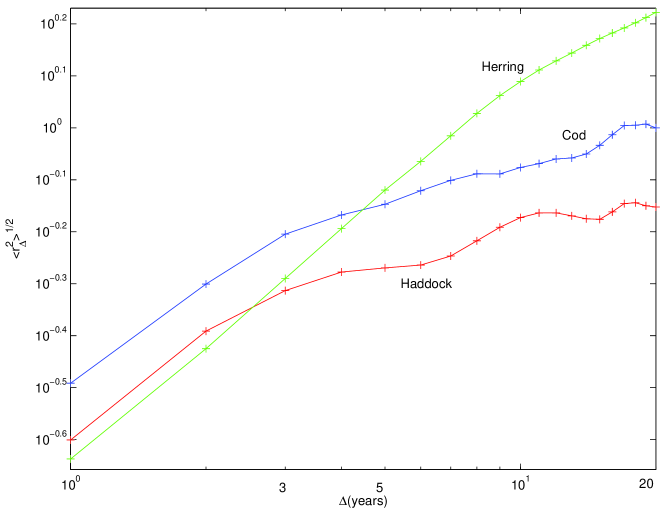
One sees that at the species level the geometrical Brownian motion is not a good hypothesis. Even for Herring, where the data seems to follow a scaling law, the slope at large $\Delta$ is closer to $0.7$ than to $0.5$. The conclusion is that whatever is actually determining the stochastic process for each species is somehow washed out when averaging over all the 27 species as Niwa did.

Actually this is no surprise. Recall the stochastic analysis result (13). To find a process $r\left(t\right)$ that has features close to Brownian motion, but is not exactly Brownian motion only means that the process is square-integrable with respect to the (Wiener) measure generated by Brownian motion. All the interesting features actually lie on the dynamics of the process $\sigma\left(t\right)$. That is, on the dynamics of the amplitude of the fluctuations. In fact this makes sense in biological terms because it is known [14] [15] that fishing magnifies fluctuations in exploited species.

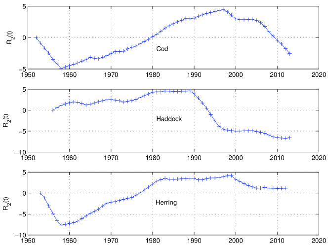
To reconstruct the dynamics of $\sigma\left(t\right)$ from the data we use a standard technique. First using a small time window we compute the local value of $\sigma\left(t\right)$ by the standard deviation of $r\left(t\right)$. For the numerical results presented here a window of $6$ years has been used. Then form the cumulative processes

$$\sum_{i=1}^{t}\sigma\left(i\right) = \beta_{1}t+R_{1}\left(t\right)$$

$$\sum_{i=1}^{t}\ln\sigma\left(i\right) = \beta_{2}t+R_{2}\left(t\right)$$ (24)

$\beta_{1}$ and $\beta_{2}$ being the average values of $\sigma$ and $\ln\sigma$ and $R_{1}$ and $R_{2}$ the cumulative processes of the fluctuations about the average. To obtain a model for the fluctuations one looks for the scaling properties of $R_{1}$ and $R_{2}$, namely the behavior of $\mathbb{E}\left|R_{1}\left(t\right)-R_{1}\left(t+\Delta\right)\right|$ and $\mathbb{E}\left|R_{2}\left(t\right)-R_{2}\left(t+\Delta\right)\right|$ as a function of the time lag $\Delta$.

Figure 3: The scaling behavior of $R_{1}$

Figure 4: The scaling behavior of $R_{2}$

The conclusion is that although not perfect, which would not be expected with data covering at most 68 points, we may assume that $R_{1}$ and $R_{2}$ obey an approximate scaling law with exponents $H$ in the range $0.8-0.9$. Therefore $R_{1}$ and $R_{2}$ may be modelled by fractional Brownian motion implying that the fluctuations of $\sigma$ and $\ln\sigma$, away from an average value, are modeled by Gaussian fractional noise. We have looked for scaling both for the cumulative $\sigma$ and $\ln\sigma$ to decide which one would provide a simpler model for the amplitude fluctuations. However, with the data available, there is no clear decision. Therefore two alternative models are proposed for the population fluctuations

$$dS\left(t\right) = \sigma\left(t\right)S\left(t\right)dB_{t}$$

$$\sigma\left(t\right) = \beta_{1}+\alpha_{1}\left(B_{H_{1}}\left(t\right)-B_{H_{1}}\left(t-1\right)\right)$$ (25)

or

$$dS\left(t\right) = \sigma\left(t\right)S\left(t\right)dB_{t}$$

$$\ln\sigma\left(t\right) = \beta_{2}+\alpha_{2}\left(B_{H_{2}}\left(t\right)-B_{H_{2}}\left(t-1\right)\right)$$ (26)

From the data the following values are obtained for the Hurst coefficients $H_{1}$ and $H_{2}$

	$H_{1}$	$H_{2}$
Cod	$0.86$	$0.87$
Haddock	$0.89$	$0.9$
Herring	$0.93$	$0.87$

From the $H-$values one sees that the dynamics of the fluctuations is a long range memory process. In addition we have found out that the processes seem to be species-dependent. For illustration we plot the cumulative amplitude fluctuations $R_{1}$ $R_{2}$ in the Figs.5 and 6.

Figure 5: Dynamics of the cumulative fluctuations of $\sigma\left(t\right)$

Figure 6: Dynamics of the cumulative fluctuations of $\ln\sigma\left(t\right)$

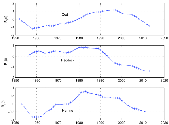
Processes with such high $H$ values are almost deterministic processes. This is an important outcome because they may provide clues on the causes of that particular dynamics.

In conclusion, this methodology of separation of the pure random features from the non-trivial dynamics of amplitude fluctuations may be useful for the analysis of other natural processes. In fact it has a solid mathematical basis as a consequence of the stochastic analysis result mentioned in (13). The dynamics of exploited fish populations provides a good example of a phenomenon where the long range dependence features appear not at the level of second order correlations but only through the analysis of higher order effects.

4 Discussion

1 - Our paper was motivated by the concerns raised in Niwa [12] that population variability corresponds to a geometric random walk and, consequently, the exploited population trajectory is a series of of random uncorrelated abundances over time. The annual change of population abundance is the result of many “shocks”, including recruitment variability, natural mortality (e.g. predation and competition) and varying fishing pressure. Despite these collection of independent drivers our results suggests that each fish stock dynamics exhibit long range dependence. Moreover, from the empirically found $H$-values associated to the fluctuations, one sees that the long range memory process seems to be species dependent. This is the reason leading to Niwa’s random walk conclusion because, when averaging over species, the $\sigma\left(t\right)$ process in Eqs. (25) and (26) would be simply replaced by a fixed number $\overline{\sigma\left(t\right)}$ (the average of $\sigma\left(t\right)$).

2 - A full discussion of whatever is actually determining the stochastic process for each species is beyond the scope of this study but the question why fish populations fluctuate has generated much attention from fishery scientists and marine ecologists over the past century. Three general hypotheses have been proposed to answer this question: (i) species interactions generate fluctuating and cyclic population dynamics; (ii) nonlinearity in single-species dynamics generates deterministic fluctuations; and (iii) changes in the environment determines variation in vital rates and recruitment, which in turn drive variation in abundance [17] [15] [20]. These are not mutually exclusive hypotheses as all three could act together to increase variability. For exploited species, fishing can also vary from year to year and translate directly into population variability or could interact with the other drivers to enhance fluctuations in fish abundance [15] [18].

Long range trends are frequently related to external forcing on the populations and are usually derived from human exploitation or environmental change. The dependence in the population growth observed for the haddock, herring and cod stocks could be derived from the different and varying exploitation regimes and/or from large-scale environmental changes as the North Atlantic Oscillation, that can induce low (or high) productivity regimes in fish recruitment (e.g. [16] [22] [23]).

Bjørnstad et al. [10] have shown that short-term variability in recruitment caused by environmental change, combined with intercohort interactions can be echoed through the population age structure inducing persistent cycles and long-term fluctuations. It is also known [21] that noise in recruitment combined with a large number of classes of spawners could lead to long-term variations in spawning stock biomass and yields, as well as to regular cycles, depending on the lifespan of the species. Furthermore, the stocks analyzed here showed species specific stochastic processes that should be analyzed considering the contrasting life history traits. The distinct growth rates, age at maturity, spawning duration and lifespan are characteristics that make some fish stocks more or less vulnerable to exploitation and environmental conditions [15] [19]. The small bodied and younger herring population should be less able to smooth out environmental fluctuations and more prone to exhibit unstable dynamics due to changing demographic parameters.

3 - There is no doubt that fisheries management would profit from a clearer understanding of the mechanisms determining the dynamics of the amplitude of the fluctuations in exploited fish stocks. The failure of many fish stocks, despite the implemented management measures, to recover rapidly to former levels of abundance, might arguably be related to the long range memory observed in this study. However, acknowledging the uncertainty arising from the reduced number of species analyzed stresses the importance of retaining more time series of population abundance over long periods, if the aim is to detect and describe the underlying mechanisms that drive population variability.

References

- [1] G. Samorodnitsky; Long Range Dependence, Foundations and Trends in Stochastic Systems 1 (2006) 163–257.
- [2] G. Dominique; How can we define the concept of long memory? An econometric survey, Econometric reviews 24 (2005) 113–149.
- [3] P. Doukhan, G. Oppenheim, and M. S. Taqqu; Theory and Applications of Long-Range Dependence, Springer, Berlin 2003.
- [4] G. Samorodnitsky and M. S. Taqqu; Stable non-Gaussian processes: Stochastic models with infinite variance, Chapman and Hall, New York 1994.
- [5] D. Nualart; The Malliavin calculus and related topics, Springer, Berlin 2006.
- [6] C. Granger and R. Joyeux; An introduction to long-memory time series and fractional differencing, J. of Time Series Analysis 1 (1980) 15-30.
- [7] J. Hosking; Fractional differencing, Biometrika 68 (1981) 165-176.
- [8] R. Bradley; Basic properties of strong mixing conditions. A survey and some open questions, Probability Surveys 2 (2005) 107-144.
- [9] R. Dickson and K. Brander; Effects of a changing windfield on cod stocks of the North Atlantic, Fisheries Oceanography 2 (1993)124-153.
- [10] O. Bjørnstad, J. M. Fromentin, N. C. Stenseth and J. Gjøsæter; Cycles and trends in cod populations, Proceedings of the National Academy of Sciences USA, 96 (1999) 5066–5071.
- [11] J. M. Fromentin, R. M. Myers, O. Bjørnstad, N. C. Stenseth, J. Gjøsæter and H. Christie; Effects of density-dependent and stochastic processes on the stabilization of cod populations, Ecology 82 (2001) 567–579.
- [12] H.-S. Niwa; Random-walk dynamics of exploited fish populations, ICES Journal of Marine Science, 64 (2007) 496–502.
- [13] http://www.ices.dk/community/advisory-process/Pages/Latest-Advice.aspx
- [14] C.-h. Hsieh, C. S. Reiss, J. R. Hunter, J. R. Beddington, R. M. May and G. Sugihara; Fishing elevates variability in the abundance of exploited species, Nature 443 (2006) 859-862.
- [15] C. N. K. Anderson, C.-h. Hsieh, S. A. Sandin, R. Hewitt, A. Hollowed, J. Beddington, R. S. May and G. Sugihara; Why fishing magnifies fluctuations in fish abundance, Nature 452 (2008) 835-839.
- [16] C. S. Leif, G. Ottersen, K. Brander, K. Chan and N. C. Stenseth; Cod and climate: effect of the North Atlantic Oscillation on recruitment in the North Atlantic, Marine Ecology Progress Series 325 (2006) 227–241.
- [17] A. O. Shelton and M. Mangel; Fluctuations of fish populations and the magnifying effects of fishing. Proceedings of the National Academy of Sciences USA, 108 (2011)7075–7080.
- [18] P. Turchin and A. D. Taylor; Complex dynamics in ecological time series. Ecology 73 (1992) 289–305.
- [19] J. Reynolds, S. Jennings and N. K. Dulvy; Life histories of fishes and population responses to exploitation, In : Conservation of Exploited Species pp. 147-168, J. D. Reynolds, G. M. Mace, K. H. Redford and J. G. Robinson (eds.), Cambridge University Press, Cambridge 2001.
- [20] J. E. Overland, J. Alheit, A. Bakun, J. W. Hurrell, D. L. Mackas and A. J. Miller; Climate controls on marine ecosystems and fish populations, Journal of Marine Systems 79 (2010) 305–315.
- [21] J. Fromentin and A. Fonteneau; Fishing effects and life history traits: a case study comparing tropical versus temperate tunas. Fisheries Research 53 (2001) 133-150.
- [22] M. F. Borges, H. C. Mendes and A. M. P. Santos; Sardine (Sardina pilchardus) recruitment is strongly affected by climate even at high spawning biomass in West Iberia/Canary upwelling system in Science and Management of Small Pelagics, S. Garcia, M. Tandstad and A. M. Caramelo (eds.), FAO Fisheries and Aquaculture Proceedings 18 (2011) 237-244.
- [23] K. Brander; Cod recruitment is strongly affected by climate when stock biomass is low, ICES Journal of Marine Science 62 (2005) 339-343.