On a class of matrix pencils and $\ell$-ifications equivalent to a given matrix polynomial

Abstract

A new class of linearizations and $\ell$-ifications for $m\times m$ matrix polynomials $P(x)$ of degree $n$ is proposed. The $\ell$-ifications in this class have the form $A(x)=D(x)+(e\otimes I_{m})W(x)$ where $D$ is a block diagonal matrix polynomial with blocks $B_{i}(x)$ of size $m$, $W$ is an $m\times qm$ matrix polynomial and $e=(1,\ldots,1)^{t}\in\mathbb{C}^{q}$, for a suitable integer $q$. The blocks $B_{i}(x)$ can be chosen a priori, subjected to some restrictions. Under additional assumptions on the blocks $B_{i}(x)$ the matrix polynomial $A(x)$ is a strong $\ell$-ification, i.e., the reversed polynomial of $A(x)$ defined by $A^{\#}(x):=x^{\deg A(x)}A(x^{-1})$ is an $\ell$-ification of $P^{\#}(x)$. The eigenvectors of the matrix polynomials $P(x)$ and $A(x)$ are related by means of explicit formulas. Some practical examples of $\ell$-ifications are provided. A strategy for choosing $B_{i}(x)$ in such a way that $A(x)$ is a well conditioned linearization of $P(x)$ is proposed. Some numerical experiments that validate the theoretical results are reported.

AMS classification: 65F15, 15A21, 15A03
Keywords: Matrix polynomials, matrix pencils, linearizations, companion matrix, tropical roots.

1 Introduction

A standard way to deal with an $m\times m$ matrix polynomial $P(x)=\sum_{i=0}^{n}P_{i}x^{i}$ is to convert it to a linear pencil, that is to a linear matrix polynomial of the form $L(x)=Ax-B$ where $A$ and $B$ are $mn\times mn$ matrices such that $\det P(x)=\det L(x)$. This process, known as linearization, has been considered in [17].

In certain cases, like for matrix polynomials modeling Non-Skip-Free stochastic processes [4], it is more convenient to reduce the matrix polynomial to a quadratic polynomial of the form $Ax^{2}+Bx+C$, where $A,B,C$ are matrices of suitable size [4]. The process that we obtain this way is referred to as quadratization. If $P(x)$ is a matrix power series, like in M/G/1 Markov chains [25, 26], the quadratization of $P(x)$ can be obtained with block coefficients of infinite size [28]. In this framework, the quadratic form is desirable since it is better suited for an effective solution of the stochastic model; in fact it corresponds to a QBD process for which there exist efficient solution algorithms [4], [22]. In other situations it is preferable to reduce the matrix polynomial $P(x)$ of degree $n$ to a matrix polynomial of lower degree $\ell$. This process is called $\ell$-ification in [15].

Techniques for linearizing a matrix polynomial have been widely investigated. Different companion forms of a matrix polynomial have been introduced and analyzed, see for instance [2, 14, 24] and the literature cited therein. A wide literature exists on matrix polynomials with contribution of many authors [1, 10, 12, 13, 14, 17, 19, 20, 21, 30, 33], motivated both by the theoretical interest of this subject and by the many applications that matrix polynomials have [4, 22, 23, 25, 25, 32]. Techniques for reducing a matrix polynomial, or a matrix power series into quadratic form, possibly with coefficients of infinite size, have been investigated in [4, 28]. Reducing a matrix polynomial to a polynomial of degree $\ell$ is analyzed in [15].

Denote by $\mathbb{C}[x]^{m\times m}$ the set of $m\times m$ matrix polynomials over the complex field $\mathbb{C}$. If $P(x)=\sum_{i=0}^{n}P_{i}x^{i}\in\mathbb{C}[x]^{m\times m}$ and $P_{n}\neq 0$ we say that $P(x)$ has degree $n$. If $\det P(x)$ is not identically zero we say that $P(x)$ is regular. Throughout the paper we assume that $P(x)$ is a regular polynomial of degree $n$. The following definition is useful in our framework.

Definition 1.

Let $P(x)\in\mathbb{C}[x]^{m\times m}$ be a matrix polynomial of degree $n$. Let $q$ be an integer such that $0<q\leq n$. We say that a matrix polynomial $Q(x)\in\mathbb{C}[x]^{qm\times qm}$ is equivalent to $P(x)$, and we write $P(x)\approx Q(x)$ if there exist two matrix polynomials $E(x),F(x)\in\mathbb{C}[x]^{qm\times qm}$ such that $\det E(x)$ and $\det F(x)$ are nonzero constants, that is $E(x)$ and $F(x)$ are unimodular, and

$$E(x)Q(x)F(x)=\begin{bmatrix}I_{m(q-1)}&0\\ 0&P(x)\\ \end{bmatrix}=:I_{m(q-1)}\oplus P(x).$$

Denote $P^{\#}(x)=x^{n}P(x^{-1})$ the reversed polynomial obtained by reverting the order of the coefficients. We say that the polynomials $P(x)$ and $Q(x)$ are strongly equivalent if $P(x)\approx Q(x)$ and $P^{\#}(x)\approx Q^{\#}(x)$. If the degree of $Q(x)$ is 1 and $P(x)\approx Q(x)$ we say that $Q(x)$ is a linearization of $P(x)$. Similarly, we say that $Q(x)$ is a strong linearization if $Q(x)$ is strongly equivalent to $P(x)$ and $\deg Q(x)=1$. If $Q(x)$ has degree $\ell$ we use the terms $\ell$-ification and strong $\ell$-ification.

It is clear from the definition that $P(x)\approx Q(x)$ implies $\det P(x)=\kappa\det Q(x)$ where $\kappa$ is some nonzero constant, but the converse is not generally true. The equivalence property is actually stronger because it preserves also the eigenstructure of the matrix polynomial, and not only the eigenvalues. For a more in-depth view of this subject see [15].

In the literature, a number of different linearizations have been proposed. The most known are probably the Frobenius and the Fiedler linearizations [13]. One of them is, for example,

$$xA-B=x\begin{bmatrix}I_{m}&&&\\ &\ddots&&\\ &&I_{m}&\\ &&&P_{n}\\ \end{bmatrix}-\begin{bmatrix}&&&-P_{0}\\ I_{m}&&&-P_{1}\\ &\ddots&&\vdots\\ &&I_{m}&-P_{n-1}\\ \end{bmatrix},$$ (1)

where $I_{m}$ denotes the identity matrix of size $m$.

1.1 New contribution

In this paper we provide a general way to transform a given $m\times m$ matrix polynomial $P(x)=\sum_{i=0}^{n}P_{i}x^{i}$ of degree $n$ into a strongly equivalent matrix polynomial $A(x)$ of lower degree $\ell$ and larger size endowed with a strong structure. The technique relies on representing $P(x)$ with respect to a basis of matrix polynomials of the form $C_{i}(x)=\prod_{j=1,\,j\neq i}^{q}B_{j}(x)$, $i=1,\ldots,q$, where $B_{i}(x)$ such that $\deg B_{i}(x)=d_{i}$ satisfy the following requirements:

1. For every $i,j$, $B_{i}(x)B_{j}(x)-B_{j}(x)B_{i}(x)=0$, i.e., the $B_{i}(x)$ commute;

2. $B_{i}(x)$ and $B_{j}(x)$ are right coprime for every $i\neq j$. This implies that there exist $\alpha_{i,j}(x)$, $\beta_{i,j}(x)$ appropriate matrix polynomials such that $B_{i}(x)\alpha_{i,j}(x)+B_{j}(x)\beta_{i,j}(x)=I$.

The above conditions are sufficient to obtain an $\ell$-ification. In order to provide a strong $\ell$-ification, we need the following additional assumptions

1. $\deg B_{i}(x)=d$ for $i=1,\ldots,q$;

2. $B_{i}^{\#}(x)$ and $B_{j}^{\#}(x)$ are right coprime for every $i\neq j$.

According to the choice of the basis we arrive at different $\ell$-ifications $A(x)$, where $\ell\geq\lceil n/q\rceil$ is determined by the degree of the $B_{i}(x)$, represented as a $q\times q$ block diagonal matrix with $m\times m$ blocks plus a matrix of rank at most $m$.

Moreover, we provide an explicit version of right and left eigenvectors of $A(x)$ in the general case.

An example of $\ell$-ification $A(x)$ is given by

$$\begin{split}&A(x)=D(x)+(e\otimes I_{m})[W_{1},\ldots,W_{q}],\\ &D(x)=\mathop{\operator@font diag}\nolimits(B_{1}(x),\ldots,B_{q}(x)),\quad e=(1,\ldots,1)^{t}\in\mathbb{C}^{q},\\ &B_{i}(x)=b_{i}(x)I_{m},\leavevmode\nobreak\ \leavevmode\nobreak\ \hbox{for }i=1,\ldots,q-1,\\ &B_{q}(x)=b_{q}(x)P_{n}+sI_{m},\leavevmode\nobreak\ \leavevmode\nobreak\ d_{q}=\deg b_{q}(x),\\ &W_{i}(x)\in\mathbb{C}[x]^{m\times m},\quad\deg W_{i}(x)<\deg B_{i}(x),\end{split}$$

where $b_{1}(x),\ldots,b_{q}(x)$ are pairwise co-prime monic polynomials of degree $d_{1},\ldots,d_{q}$, respectively, such that $n=d_{1}+\cdots+d_{q}$, and $s$ is such that $\lambda b_{q}(\xi)+s\neq 0$ for any eigenvalue $\lambda$ of $P_{n}$ and for any root $\xi$ of $b_{i}(x)$ for $i=1,\ldots,q-1$. The matrix polynomial $A(x)$ has degree $\ell=\max\{d_{1},\dots,d_{q}\}\geq\lceil\frac{n}{q}\rceil$ and size $mq\times mq$.

If $b_{i}(x)=x-\beta_{i}$ are linear polynomials then $\deg A(x)=1$ and the above equivalence turns into a strong linearization, moreover the eigenvalues of $P(x)$ can be viewed as the generalized eigenvalues of the matrix pencil $A(x)$

$$A(x)=x\begin{bmatrix}I\\ &\ddots\\ &&I\\ &&&P_{n}\end{bmatrix}-\begin{bmatrix}\beta_{1}I\\ &\ddots\\ &&\beta_{n-1}I\\ &&&\beta_{n}P_{n}-sI\end{bmatrix}+\begin{bmatrix}I\\ \vdots\\ \vdots\\ I\end{bmatrix}[W_{1}\ldots W_{n}]$$

where

$$W_{i}=\begin{cases}\frac{P(\beta_{i})}{\prod_{j=1,\,j\neq i}^{n-1}(\beta_{i}-\beta_{j})}((\beta_{i}-\beta_{n})P_{n}+sI_{m})^{-1}&\text{for }i<n,\\[8.61108pt] \frac{P(\beta_{n})}{\prod_{j=1}^{n-1}(\beta_{n}-\beta_{j})}-sI_{m}-s\sum_{j=1}^{n-1}\frac{W_{i}}{\beta_{n}-\beta_{j}}&\text{otherwise}.\\ \end{cases}$$ (2)

If $P(x)$ is a scalar polynomial then $\det A(x)=\prod_{i=1}^{n}(x-\beta_{i})(\sum_{j=1}^{n}\frac{W_{j}}{x-\beta_{j}}+1)$ so that the eigenvalue problem can be rephrased in terms of the secular equation $\sum_{j=1}^{n}\frac{W_{j}}{x-\beta_{j}}+1=0$. Motivated by this fact, we will refer to this linearization as secular linearization.

Observe that this kind of linearization relies on the representation of $P(x)-\prod_{i=1}^{n}B_{i}(x)$ in the Lagrange basis formed by $C_{i}(x)=\prod_{j=1,\,j\neq i}^{n}B_{j}(x)$, $i=1,\ldots,n$ which is different from the linearization given in [2] where the pencil $A(x)$ has an arrowhead structure. Unlike the linearization of [2], our linearization does not introduce eigenvalues at infinity.

This secular linearization has some advantages with respect to the Frobenius linearization (1). For a monic matrix polynomial we show that with the linearization obtained by choosing $\beta_{i}=\omega_{n}^{i}$, where $\omega_{n}$ is a principal $n$th root of 1, our linearization is unitarily similar to the block Frobenius pencil associated with $P(x)$. By choosing $\beta_{i}=\alpha\omega_{n}^{i}$, we obtain a pencil unitarily similar to the scaled Frobenius one. With these choices, the eigenvalues of the secular linearization have the same condition number as the eigenvalues of the (scaled) Frobenius matrix.

This observation leads to better choices of the nodes $\beta_{i}$ performed according to the magnitude of the eigenvalues of $P(x)$. In fact, by using the information provided by the tropical roots in the sense of [6], we may compute at a low cost particular values of the nodes $\beta_{i}$ which greatly improve the condition number of the eigenvalues. From an experimental analysis we find that in most cases the conditioning of the eigenvalues of the linearization obtained this way is lower by several orders of magnitude with respect to the conditioning of the eigenvalues of the Frobenius matrix even if it is scaled with the optimal parameter.

Our experiments, reported in Section 6 are based on some randomly generated polynomials and on some problems taken from the repository NLEVP [3].

We believe that the information about the tropical roots, used in [16] for providing better numerically conditioned problems, can be more effectively used with our $\ell$-ification. This analysis is part of our future work.

Another advantage of this representation is that any matrix in the form “diagonal plus low-rank” can be reduced to Hessenberg form $H$ by means of Givens rotation with a low number of arithmetic operations provided that the diagonal is real. Moreover, the function $p(x)=\det(xI-H)$ as well as the Newton correction $p(x)/p^{\prime}(x)$ can be computed in $O(nm^{2})$ operations [8]. This fact can be used to implement the Aberth iteration in $O(n^{2}m^{3})$ ops instead of $O(nm^{4}+n^{2}m^{3})$ of [5]. This complexity bound seems optimal in the sense that for each one of the $mn$ eigenvalues all the $m^{2}(n+1)$ data are used at least once.

The paper is organized as follows. In Section 2 we provide the reduction of any matrix polynomial $P(x)$ to the equivalent form

$$A(x)=D(x)+(e\otimes I_{m})[W_{1}(x),\ldots,W_{q}(x)],$$

that is, the $\ell$-ification of $P(x)$. In Section 2.1 we show that $P(x)$ is strongly equivalent to $A(x)$ in the sense of Definition 1. In Section 3 we provide the explicit form of left and right eigenvectors of $A(x)$ relating them to the corresponding eigenvectors of $P(x)$. In Section 4 we analyze the case where $B_{i}(x)=b_{i}(x)I$ for $i=1,\ldots,q-1$ and $B_{q}(x)=b_{q}(x)P_{n}+sI$ for scalar polynomials $b_{i}(x)$. Section 5 outlines an algorithm for computing the $\ell$-ifications. Finally, in Section 6 we present the results of some numerical experiments.

2 A diagonal plus low rank $\ell$-ification

Here we recall a known companion-like matrix for scalar polynomials represented as a diagonal plus a rank-one matrix, provide a more general formulation and then extend it to the case of matrix polynomials. This form was introduced by B.T. Smith in [29], as a tool for providing inclusion regions for the zeros of a polynomial, and used by G.H. Golub in [18] in the analysis of modified eigenvalue problems.

Let $p(x)=\sum_{i=0}^{n}p_{i}x^{i}$ be a polynomial of degree $n$ with complex coefficients, assume $p(x)$ monic, i.e., $p_{n}=1$, consider a set of pairwise different complex numbers $\beta_{1},\ldots,\beta_{n}$ and set $e=(1,\ldots,1)^{t}$. Then it holds that [18], [29]

$$\begin{split}&p(x)=\det(xI-D+ew^{t}),\\ &D=\mathop{\operator@font diag}\nolimits(\beta_{1},\ldots,\beta_{n}),\quad w=(w_{i}),\leavevmode\nobreak\ w_{i}=\frac{p(\beta_{i})}{\prod_{j\neq i}(\beta_{i}-\beta_{j})}.\end{split}$$ (3)

Now consider a monic polynomial $b(x)$ of degree $n$ factored as $b(x)=\prod_{i=1}^{q}b_{i}(x)$, where $b_{i}(x)$, $i=1,\ldots,q$ are monic polynomials of degree $d_{i}$ which are co-prime, that is, $\gcd(b_{i}(x),b_{j}(x))=1$ for $i\neq j$, where $\gcd$ denotes the monic greatest common divisor. Recall that given a pair $u(x),v(x)$ of polynomials there exist unique polynomials $s(x),r(x)$ such that $\deg s(x)<\deg v(x)$, $\deg r(x)<\deg u(x)$, and $u(x)s(x)+v(x)r(x)=\gcd(u(x),v(x))$. From this property it follows that if $u(x)$ and $v(x)$ are co-prime, there exists $s(x)$ such that $s(x)u(x)\equiv 1\mod v(x)$. This polynomial can be viewed as the reciprocal of $u(x)$ modulo $v(x)$. Here and hereafter we denote $u(x)\mod v(x)$ the remainder of the division of $u(x)$ by $v(x)$.

This way, we may uniquely represent any polynomial of degree $n$ in terms of the generalized Lagrange polynomials $c_{i}(x)=b(x)/b_{i}(x)$, $i=1,\ldots,q$ as follows.

Lemma 2.

Let $b_{i}(x)$, $i=1,\ldots,q$ be co-prime monic polynomials such that $\deg b_{i}(x)=d_{i}$ and $b(x)=\prod_{i=1}^{q}b_{i}(x)$ has degree $n$. Define $c_{i}(x)=b(x)/b_{i}(x)$. Then there exist polynomials $s_{i}(x)$ such that $s_{i}(x)c_{i}(x)\equiv 1\mod b_{i}(x)$, moreover, any monic polynomial $p(x)$ of degree $n$ can be uniquely written as

$$\begin{split}&p(x)=b(x)+\sum_{i=1}^{q}w_{i}(x)c_{i}(x),\\ &w_{i}(x)\equiv p(x)s_{i}(x)\mod b_{i}(x),\quad i=1,\ldots,q,\end{split}$$ (4)

where $\deg w_{i}(x)<d_{i}$.

Proof.

Since $\gcd(b_{i}(x),b_{j}(x))=1$ for $i\neq j$ then $b_{i}(x)$ and $c_{i}(x)=\prod_{j\neq i}b_{j}(x)$ are co-prime. Therefore there exists $s_{i}(x)\equiv 1/c_{i}(x)\mod b_{i}(x)$. Moreover, setting $w_{i}(x)\equiv p(x)s_{i}(x)\mod b_{i}(x)$ for $i=1,\ldots,q$, it turns out that the equation $p(x)=b(x)+\sum_{i=1}^{q}w_{i}(x)c_{i}(x)$ is satisfied modulo $b_{i}(x)$ for $i=1,\ldots,q$. For the primality of $b_{1}(x),\ldots,b_{q}(x)$, this means that the polynomial $\psi(x):=p(x)-b(x)-\sum_{i=1}^{q}w_{i}(x)c_{i}(x)$ is a multiple of $\prod_{i=1}^{q}b_{i}(x)$ which has degree $n$. Since $\psi(x)$ has degree at most $n-1$ it follows that $\psi(x)=0$. That is (4) provides a representation of $p(x)$. This representation is unique since another representation, say, given by $\tilde{w}_{i}(x)$, $i=1,\ldots,q$, would be such that $\sum_{i=1}^{q}(\tilde{w}_{i}(x)-w_{i}(x))c_{i}(x)=0$, whence $(\tilde{w}_{i}(x)-w_{i}(x))c_{i}(x)\equiv 0\mod b_{i}(x)$. That is, for the co-primality of $b_{i}(x)$ and $c_{i}(x)$, the polynomial $\tilde{w}_{i}(x)-w_{i}(x)$ would be multiple of $b_{i}(x)$. The property $\deg(b_{i}(x))<\deg(\tilde{w}_{i}(x)-w_{i}(x))$ implies that $\tilde{w}_{i}(x)-w_{i}(x)=0$. ∎

The polynomial $p(x)$ in Lemma 2 can be represented by means of the determinant of a (not necessarily linear) matrix polynomial as expressed by the following result which provides a generalization of (3)

Theorem 3.

Under the assumptions of Lemma 2 we have

$$p(x)=\det A(x),\quad A(x)=D(x)+e[w_{1}(x),\ldots,w_{q}(x)]$$

for $D=\mathop{\operator@font diag}\nolimits(b_{1}(x),\ldots,b_{q}(x))$ and $e=[1,\ldots,1]^{t}$.

Proof.

Formally, one has $A(x)=D(x)(I+D(x)^{-1}e[w_{1}(x),\ldots,w_{q}(x)])$ so that

$$\begin{split}\det A(x)&=\det D(x)\det(I_{q}+D(x)^{-1}e[w_{1}(x),\ldots,w_{q}(x)])\\ &=b(x)(1+[w_{1}(x),\ldots,w_{q}(x)]D(x)^{-1}e),\end{split}$$

where $b(x)=\prod_{i=1}^{q}b_{i}(x)$. Whence, we find that $\det A(x)=b(x)+\sum_{i=1}^{q}w_{i}(x)c_{i}(x)=p(x)$, where the latter equality holds in view of Lemma 2. ∎

Observe that for $d_{i}=1$ the above result reduces to (3) where $w_{i}$ are constant polynomials. From the computational point of view, the polynomials $w_{i}(x)$ are obtained by performing a polynomial division since $w_{i}(x)$ is the remainder of the division of $p(x)s_{i}(x)$ by $b_{i}(x)$.

2.1 Strong $\ell$-ifications for matrix polynomials

The following technical Lemma is needed to prove the next Theorem 6.

Lemma 4.

Let $B_{1}(x),B_{2}(x)\in\mathbb{C}[x]^{m\times m}$ be regular and such that $B_{1}(x)B_{2}(x)=B_{2}(x)B_{1}(x)$. Assume that $B_{1}(x)$ and $B_{2}(x)$ are right co-prime, that is, there exist $\alpha(x),\beta(x)\in\mathbb{C}[x]^{m\times m}$ such that $B_{1}(x)\alpha(x)+B_{2}(x)\beta(x)=I_{m}.$ Then the $2\times 2$ block-matrix polynomial $F(x)=\left[\begin{smallmatrix}\alpha(x)&B_{2}(x)\\ -\beta(x)&B_{1}(x)\\ \end{smallmatrix}\right]$ is unimodular.

Proof.

From the decomposition

$$\begin{bmatrix}I_{m}&0\\ B_{1}(x)&-B_{2}(x)\\ \end{bmatrix}\begin{bmatrix}\alpha(x)&B_{2}(x)\\ -\beta(x)&B_{1}(x)\\ \end{bmatrix}=\begin{bmatrix}\alpha(x)&B_{2}(x)\\ I_{m}&0\\ \end{bmatrix}$$

we have $-\det B_{2}(x)\det F(x)=-\det B_{2}(x)$. Since $B_{2}(x)$ is regular then $\det F(x)=1$. ∎

Lemma 5.

Let $P(x),Q(x)$ and $T(x)$ be pairwise commuting right co-prime matrix polynomials. Then $P(x)Q(x)$ and $T(x)$ are also right co-prime.

Proof.

We know that there exists $\alpha_{P}(x),\beta_{P}(x),\alpha_{Q}(x),\beta_{Q}(x)$, matrix polynomials such that

$$P(x)\alpha_{P}(x)+T(x)\beta_{P}(x)=I,\quad Q(x)\alpha_{Q}(x)+T(x)\beta_{Q}(x)=I.$$

We shall prove that there exist appropriate $\alpha(x),\beta(x)$ matrix polynomials such that $P(x)Q(x)\alpha(x)+T(x)\beta(x)=I$. We have

$$P(x)Q(x)(\alpha_{Q}(x)\alpha_{P}(x))+T(x)(P(x)\beta_{Q}(x)\alpha_{P}(x)+\beta_{P}(x))=$$

$$P(x)(Q(x)\alpha_{Q}(x)+T(x)\beta_{Q}(x))\alpha_{P}(x)+T(x)\beta_{P}(x)=$$

$$P(x)\alpha_{P}(x)+T(x)\beta_{P}(x)=I,$$

where the first equality holds since $T(x)P(x)=P(x)T(x)$. So we can conclude that also $P(x)Q(x)$ and $T(x)$ are right coprime, and a possible choice for $\alpha(x)$ and $\beta(x)$ is:

$$\alpha(x)=\alpha_{Q}(x)\alpha_{P}(x),\qquad\beta(x)=P(x)\beta_{Q}(x)\alpha_{P}(x)+\beta_{P}(x).$$

∎

Now we are ready to prove the main result of this section, which provides an $\ell$-ification of a matrix polynomial $P(x)$ which is not generally strong. Conditions under which this $\ell$-ification is strong are given in Theorem 8.

Theorem 6.

Let $P(x)=\sum_{i=0}^{n}P_{i}x^{i}$, $B_{1}(x),\ldots,B_{q}(x)$, and $W_{1}(x),\ldots,W_{q}(x)$ be polynomials in $\mathbb{C}[x]^{m\times m}$. Let $C_{i}(x)=\prod_{\begin{subarray}{c}j=1,\,\end{subarray}{j\neq i}}^{q}B_{j}(x)$ and suppose that the following conditions hold:

1. $P(x)=\prod_{i=1}^{q}B_{i}(x)+\sum_{i=1}^{q}W_{i}(x)C_{i}(x)$;

2. the polynomials $B_{i}(x)$ are regular, commute, i.e., $B_{i}(x)B_{j}(x)-B_{j}(x)B_{i}(x)=0$ for any $i,j$, and are pairwise right co-prime.

Then the matrix polynomial $A(x)$ defined as

$$A(x)=D(x)+(e\otimes I_{m})[W_{1}(x),\ldots,W_{q}(x)],\leavevmode\nobreak\ D(x)=\mathop{\operator@font diag}\nolimits(B_{1}(x),\ldots,B_{q}(x))$$ (5)

is equivalent to $P(x)$, i.e., there exist unimodular $q\times q$ matrix polynomials $E(x)$, $F(x)$ such that $E(x)A(x)F(x)=I_{m(q-1)}\oplus P(x)$.

Proof.

Define $E_{0}(x)$ the following (constant) matrix:

$$E_{0}(x)=\begin{bmatrix}I_{m}&-I_{m}\\ &I_{m}&-I_{m}\\ &&\ddots&\ddots\\ &&&I_{m}&-I_{m}\\ &&&&I_{m}\\ \end{bmatrix}.$$

A direct inspection shows that

$$E_{0}(x)A(x)=\begin{bmatrix}B_{1}(x)&-B_{2}(x)\\ &B_{2}(x)&-B_{3}(x)\\ &&\ddots&\ddots\\ &&&B_{q-1}(x)&-B_{q}(x)\\ W_{1}(x)&W_{2}(x)&\cdots&W_{q-1}(x)&B_{q}(x)+W_{q}(x)\\ \end{bmatrix}.$$

Using the fact that the polynomials $B_{i}(x)$ are right co-prime, we transform the latter matrix into block diagonal form. We start by cleaning $B_{1}(x)$. Since $B_{1}(x),B_{2}(x)$ are right co-prime, there exist polynomials $\alpha(x)$, $\beta(x)$ such that $B_{1}(x)\alpha(x)+B_{2}(x)\beta(x)=I_{m}.$ For the sake of brevity, from now on we write $\alpha,\beta$, $W_{i}$ and $B_{i}$ in place of $\alpha(x),\beta(x)$, $W_{i}(x)$ and $B_{i}(x)$, respectively. Observe that the matrix

$$F_{1}(x)=\begin{bmatrix}\alpha&B_{2}\\ -\beta&B_{1}\\ \end{bmatrix}\oplus I_{m(q-2)}.$$

is unimodular in view of Lemma 4, moreover

$$E_{0}(x)A(x)F_{1}(x)=\begin{bmatrix}I_{m}&\\ -B_{2}\beta&B_{1}B_{2}&-B_{3}\\ &&\ddots&\ddots\\ &&&B_{q-1}&-B_{q}\\ W_{1}\alpha-W_{2}\beta&W_{1}B_{2}+W_{2}B_{1}&\cdots&W_{m-1}&B_{q}+W_{q}\\ \end{bmatrix}.$$

Using row operations we transform to zero all the elements in the first column of this matrix (by just adding multiples of the first row to the others). That is, there exists a suitable unimodular matrix $E_{1}(x)$ such that

$$E_{1}(x)E_{0}(x)A(x)F_{1}(x)=\begin{bmatrix}I_{m}&\\ &B_{1}B_{2}&-B_{3}\\ &&\ddots&\ddots\\ &&&B_{q-1}&-B_{q}\\ &W_{2}B_{1}+W_{1}B_{2}&\cdots&W_{q-1}&B_{q}+W_{q}\\ \end{bmatrix}.$$

In view of Lemma 5, $B_{1}B_{2}$ is right coprime with $B_{3}$. Thus, we can recursively apply the same process until we arrive at the final reduction step:

$$E_{q-1}(x)\ldots E_{0}(x)A(x)F_{1}(x)\ldots F_{q-1}(x)=I_{m(q-1)}\oplus\left(\prod_{i=1}^{q}B_{i}(x)+\sum_{i=1}^{q}W_{i}(x)C_{i}(x)\right)$$

where the last diagonal block is exactly $P(x)$ in view of assumption 1. ∎

Observe that if $m=1$ and $B_{i}(x)=x-\beta_{i}$ then we find that (3) provides the secular linearization for $P(x)$.

Now, we can prove that the polynomial equivalence that we have just presented is actually a strong equivalence, under the following additional assumptions

$$\begin{split}&\deg B_{i}(x)=d,\quad i=1,\ldots,q,\\ &n=dq,\quad\deg W_{i}(x)<\deg B_{i}(x)\\ &B_{i}^{\#}(x),\hbox{ are pairwise right co-prime}.\end{split}$$ (6)

Remark 7.

Recall that, according to Theorem 7.5 of [15] in an algebraically closed field there exists a strong $\ell$-ification for a degree $n$ regular matrix polynomial $P(x)\in\mathbb{C}^{m\times m}[x]$ if and only if $\ell|nm$. Conditions (6) satisfy this requirement, since $\ell=d$ and $d|n$.

To accomplish this task we will show that the reversed matrix polynomial of $A(x)=D(x)+(e\otimes I_{m})W$, $W=[W_{1},\ldots,W_{q}]$, has the same structure as $A(x)$ itself.

Theorem 8.

Under the assumptions of Theorem 6 and of (6) the secular $\ell$-ification given in Theorem 6 is strong.

Proof.

Consider $A^{\#}(x)=x^{d}A(x^{-1})$. We have

$$A^{\#}(x)=\mathop{\operator@font diag}\nolimits(x^{d}B_{1}(x^{-1}),\ldots,x^{d}B_{q}(x^{-1}))+(e\otimes I_{m})[x^{d}W_{1}(x^{-1}),\cdots,x^{d}W_{q}(x^{-1})].$$

This matrix polynomial is already in the same form as $A(x)$ of (5) and verifies the assumptions of Theorem 6 since the polynomials $x^{d}B_{1}(x^{-1})$ are pairwise right co-prime and commute with each other in view of equation (6). Thus, Theorem 6 implies that $A^{\#}(x)$ is an $\ell$-ification for

$$\begin{split}\prod_{i=1}^{q}x^{d}B_{i}(x^{-1})&+\sum_{i=1}^{q}x^{d}W_{i}(x^{-1})\prod_{j\neq i}x^{d}B_{j}(x^{-1})\\ &=x^{dq}\left(\prod_{i=1}^{q}B_{i}(x^{-1})+\sum_{i=1}^{q}W_{i}(x^{-1})\prod_{j\neq i}B_{j}(x^{-1})\right)\\ &=x^{n}P(x^{-1})=P^{\#}(x),\end{split}$$

where the first equality follows from the fact that $n=dq$ in view of equation (6). This concludes the proof. ∎

Remark 9.

Note that in the case where the $B_{i}(x)$ do not have the same degree, the secular $\ell$-ification might not be strong: the finite eigenstructure is preserved but some infinite eigenvalues not present in $P(x)$ will be artificially introduced.

3 Eigenvectors

In this section we provide an explicit expression of right and left eigenvectors of the matrix polynomial $A(x)$.

Theorem 10.

Let $P(x)$ be a matrix polynomial, $A(x)$ its secular $\ell$-ification defined in Theorem 6, $\lambda\in\mathbb{C}$ such that $\det P(\lambda)=0$, and assume that $\det B_{i}(\lambda)\neq 0$ for all $i=1,\ldots,q$. If $v_{A}=(v_{1}^{t},\ldots,v_{q}^{t})^{t}\in\mathbb{C}^{mq}$ is such that $A(\lambda)v_{A}=0$, $v_{A}\neq 0$ then $P(\lambda)v=0$ where $v=-\prod_{i=1}^{q}B_{i}(\lambda)^{-1}\sum_{j=1}^{q}W_{j}v_{j}\neq 0$. Conversely, if $v\in\mathbb{C}^{m}$ is a nonzero vector such that $P(\lambda)v=0$, then the vector $v_{A}$ defined by $v_{i}=\prod_{j\neq i}B_{j}(\lambda)v$, $i=1,\ldots,q$ is nonzero and such that $A(\lambda)v_{A}=0$.

Proof.

Let $v_{A}\neq 0$ be such that $A(\lambda)v_{A}=0$, so that

$$B_{i}(\lambda)v_{i}+\sum_{j=1}^{q}W_{j}(\lambda)v_{j}=0,\quad i=1,\ldots,q.$$ (7)

Let $v=-(\prod_{i=1}^{q}B_{i}(\lambda)^{-1})\sum_{j=1}^{q}W_{j}(\lambda)v_{j}$. Combining the latter equation and (7) yields

$$v_{i}=-B_{i}(\lambda)^{-1}\left(\sum_{j=1}^{q}W_{j}(\lambda)v_{j}\right)=\prod_{j=1,\,j\neq i}^{q}B_{j}(\lambda)v.$$ (8)

Observe that if $v=0$ then, by definition of $v$, one has $\sum_{j=1}^{q}W_{j}(\lambda)v_{j}=0$ so that, in view of (7), we find that $B_{i}(\lambda)v_{i}=0$. Since $\det B_{i}(\lambda)\neq 0$ this would imply that $v_{i}=0$ for any $i$ so that $v_{A}=0$ which contradicts the assumptions. Now we prove that $P(\lambda)v=0$. In view of (8) we have

$$P(\lambda)v=\prod_{j=1}^{q}B_{j}(\lambda)v+\sum_{i=1}^{q}W_{i}(\lambda)\prod_{j=1,\,j\neq i}^{q}B_{j}(\lambda)v=\prod_{j=1}^{q}B_{j}(\lambda)v+\sum_{i=1}^{q}W_{i}(\lambda)v_{i}.$$

Moreover, by definition of $v$ we get

$$P(\lambda)v=-\prod_{j=1}^{q}B_{j}(\lambda)(\prod_{i=1}^{q}B_{i}(\lambda)^{-1})\sum_{i=1}^{q}W_{i}(\lambda)v_{i}+\sum_{i=1}^{q}W_{i}(\lambda)v_{i}=0.$$

Similarly, we can prove the opposite implication. ∎

A similar result can be proven for left eigenvectors. The following theorem relates left eigenvectors of $A(x)$ and left eigenvectors of $P(x)$.

Theorem 11.

Let $P(x)$ be a matrix polynomial, $A(x)$ its secular $\ell$-ification defined in Theorem 6, $\lambda\in\mathbb{C}$ such that $\det P(\lambda)=0$, and assume that $\det B_{i}(\lambda)\neq 0$. If $u_{A}^{t}=(u_{1}^{t},\ldots,u_{q}^{t})\in\mathbb{C}^{mq}$ is such that $u_{A}^{t}A(\lambda)=0$, $u_{A}\neq 0$, then $u^{t}P(\lambda)=0$ where $u=\sum_{i=1}^{q}u_{i}\neq 0$. Conversely, if $u^{t}P(\lambda)=0$ for a nonzero vector $u\in\mathbb{C}^{m}$ then $u_{A}^{t}A(\lambda)=0$, where $u_{A}$ is a nonzero vector defined by $u_{i}^{t}=-u^{t}W_{i}(\lambda)B_{i}(\lambda)^{-1}$ for $i=1,\ldots,q$.

Proof.

If $u_{A}^{t}A(\lambda)=0$ then from the expression of $A(x)$ given in Theorem 6 we have

$$u_{i}^{t}B_{i}(\lambda)+\left(\sum_{j=1}^{q}u_{j}^{t}\right)W_{i}(\lambda)=0,\quad i=1,\ldots,q.$$ (9)

Assume that $u=\sum_{j=1}^{q}u_{j}=0$. Then from the above expression we obtain, for any $i$, $u_{i}^{t}B_{i}(\lambda)=0$ that is $u_{i}=0$ for any $i$ since $\det B_{i}(\lambda)\neq 0$. This is in contradiction with $u_{A}\neq 0$. From (9) we obtain $u_{i}^{t}=-u^{t}W_{i}(\lambda)B_{i}(\lambda)^{-1}$. Moreover, multiplying (9) to the right by $\prod_{j=1,\,j\neq i}^{q}B_{j}$ yields

$$0=u_{i}^{t}\prod_{j=1}^{q}B_{j}(\lambda)+u^{t}W_{i}(\lambda)\prod_{j=1,\,j\neq i}^{q}B_{j}(\lambda).$$

Taking the sum of the above expression for $i=1,\ldots,q$ yields

$$0=\left(\sum_{i=1}^{q}u_{i}^{t}\right)\prod_{j=1}^{q}B_{j}(\lambda)+u^{t}\sum_{i=1}^{q}W_{i}(\lambda)\prod_{j=1,\,j\neq i}^{q}B_{j}(\lambda)=u^{t}P(\lambda).$$

Conversely, assuming that $u^{t}P(\lambda)=0$, from the representation

$$P(x)=\prod_{j=1}^{n}B_{j}(x)+\sum_{i=1}^{q}W_{i}(x)\prod_{j=1,\,j\neq i}^{q}B_{i}(x),$$

defining $u_{i}^{t}=-u^{t}W_{i}(\lambda)B_{i}(\lambda)^{-1}$ we obtain

$$\sum_{i=1}^{q}u_{i}^{t}=-u^{t}\sum_{i=1}^{q}W_{i}(\lambda)B_{i}(\lambda)^{-1}=-u^{t}(P(\lambda)\prod_{j=1}^{q}B_{j}(\lambda)^{-1}-I)=u^{t}$$

and therefore from (9) we deduce that $u_{A}^{t}A(\lambda)=0$. ∎

The above result does not cover the case where $\det B_{i}(\lambda)=0$ for some $i$.

3.1 A sparse $\ell$-ification

Consider the block bidiagonal matrix $L$ having $I_{m}$ on the block diagonal and $-I_{m}$ on the block subdiagonal. It is immediate to verify that $L(e\otimes I_{m})=e_{1}\otimes I_{m}$, where $e_{1}=(1,0,\ldots,0)^{t}$. This way, the matrix polynomial $H(x)=LA(x)$ is a sparse $\ell$-ification of the form

$$H(x)=\left[\begin{array}[]{ccccc}B_{1}(x)+W_{1}(x)&W_{2}(x)&\ldots&W_{q-1}(x)&W_{q}(x)\\ -B_{1}(x)&B_{2}(x)\\ &-B_{2}(x)&\ddots\\ &&\ddots&B_{q-1}(x)\\ &&&-B_{q-1}(x)&B_{q}(x)\end{array}\right]$$

4 A particular case

In the previous section we have provided (strong) $\ell$-ifications of a matrix polynomial $P(x)$ under the assumption of the existence of the representation

$$P(x)=\prod_{i=1}^{q}B_{i}(x)+\sum_{i=1}^{q}W_{i}(x)\prod_{j\neq i}B_{j}(x)$$ (10)

and under suitable conditions on $B_{i}(x)$. In this section we show that a specific choice of the blocks $B_{i}(x)$ satisfies the above assumptions and implies the existence of the representation (10). Moreover, we provide explicit formulas for the computation of $W_{i}(x)$ given $P(x)$ and $B_{i}(x)$.

We provide also some additional conditions in order to make the resulting $\ell$-ification strong.

Assumption 1.

The matrix polynomials $B_{i}(x)$ are defined as follows

$$\begin{cases}B_{i}(x)=b_{i}(x)I&i=1,\ldots,q-1\\ B_{q}(x)=b_{q}(x)P_{n}+sI&\text{otherwise}\\ \end{cases}$$

where $b_{i}(x)$ are scalar polynomials such that $\deg b_{i}(x)=d_{i}$ and $\sum_{i=1}^{q}d_{i}=n$; the polynomials $b_{i}(x)$, $i=1,\ldots,q$, are pairwise co-prime; $s$ is a constant such that $\lambda b_{q}(\xi)+s\neq 0$ for any eigenvalue $\lambda$ of $P_{n}$ and for any root $\xi$ of $b_{i}(x)$, for $i=1,\dots,q-1$.

In this case it is possible to prove the existence of the representation (10). We rely on the Chinese remainder theorem that here we rephrase in terms of matrix polynomials.

Lemma 12.

Let $b_{i}(x)$, $i=1,\ldots,q$ be co-prime polynomials of degree $d_{1},\ldots,d_{q}$, respectively, such that $\sum_{i=1}^{q}d_{i}=n$. If $P_{1}(x)$, $P_{2}(x)$ are matrix polynomials of degree at most $n-1$ then $P_{1}(x)=P_{2}(x)$ if and only if $P_{1}(x)-P_{2}(x)\equiv 0\mod b_{i}(x)$, for $i=1,\ldots,q$.

Proof.

The implication $P_{1}(x)-P_{2}(x)=0$ $\Rightarrow$ $P_{1}(x)-P_{2}(x)\equiv 0\mod b_{i}(x)$ is trivial. Conversely, if $P_{1}(x)-P_{2}(x)\equiv 0\mod b_{i}(x)$ for every $b_{i}$ then the entries of $P_{1}(x)-P_{2}(x)$ are multiples of $\prod_{i=1}^{q}b_{i}(x)$ for the co-primality of the polynomials $b_{i}(x)$. But this implies that $P_{1}(x)-P_{2}(x)=0$ since the degree of $P_{1}(x)-P_{2}(x)$ is at most $n-1$ while $\prod_{i=1}^{q}b_{i}(x)$ has degree $n$. ∎

We have the following

Theorem 13.

Let $P(x)=\sum_{i=0}^{n}x^{i}P_{i}$ be an $m\times m$ matrix polynomial over an algebraically closed field. Under Assumption 1, set $C_{i}(x)=\prod_{j\neq i}B_{j}(x)$. Then there exists a unique decomposition

$$P(x)=B(x)+\sum_{i=1}^{q}W_{i}(x)C_{i}(x),\qquad B(x)=\prod_{i=1}^{q}B_{i}(x),$$ (11)

where $W_{i}(x)$ are matrix polynomials of degree less than $d_{i}$ for $i=1,\dots,q$ defined by

$$\begin{split}&W_{i}(x)=\frac{P(x)}{\prod_{j=1,\,j\neq i}^{q-1}b_{j}(x)}(b_{q}(x)P_{n}+sI_{m})^{-1}\mod b_{i}(x),\quad i=1,\ldots,q-1\\ &W_{q}(x)=\frac{1}{\prod_{j=1}^{q-1}b_{j}(x)}P(x)-sI_{m}-s\sum_{j=1}^{q-1}\frac{W_{j}(x)}{b_{j}(x)}\mod b_{q}(x).\end{split}$$ (12)

Proof.

We show that there exist matrix polynomials $W_{i}(x)$ of degree less than $d_{i}$ such that $P(x)-B(x)\equiv\sum_{i=1}^{q}W_{i}(x)C_{i}(x)\mod b_{i}(x)$ for $i=1,\ldots,q$. Then we apply Lemma 12 with $P_{1}(x)=P(x)-B(x)$ that by construction has degree at most $n-1$, and with $P_{2}(x)=\sum_{i=1}^{q}W_{i}(x)C_{i}(x)$, and conclude that $P(x)=B(x)+\sum_{i=1}^{q}W_{i}(x)C_{i}(x)$. Since for $i=1,\ldots,q-1$ the polynomial $b_{i}(x)$ divides every entry of $B(x)$ and of $C_{j}(x)$ for $j\neq i$, we find that $P(x)\equiv W_{i}(x)C_{i}(x)\mod b_{i}(x),\quad i=1,\ldots,q.$ Moreover, for $i<q$ we have $C_{i}(x)=\left(\prod_{j\neq i,j<q}b_{j}(x)I_{m}\right)(b_{q}(x)P_{n}+sI_{m})$. The first term is invertible modulo $b_{i}(x)$ since by assumption $b_{i}(x)$ is co-prime with $b_{j}$ for every $j\neq i$. We need to prove that the matrix on the right is invertible modulo $b_{i}(x)$, that is, its eigenvalues $\mu$ are such that $b_{i}(\mu)\neq 0$. Now, since the eigenvalues of $b_{q}(x)P_{n}+sI_{m}$ have the form $\mu=b_{q}(x)\lambda+s$, where $\lambda$ is an eigenvalue of $P_{n}$, it is enough to ensure that for every $\xi$ which is a root of $b_{i}(x)$ the value $\lambda b_{q}(\xi)+s$ is different from $0$ for $i=1,\ldots,q-1$. This is guaranteed by hypothesis, and so we obtain the explicit formula for $W_{i}(x)$, $i=1,\ldots,q-1$ given by (12). It remains to find an explicit expression for $W_{q}(x)$. We have $W_{q}(x)C_{q}(x)=P(x)-\sum_{j=1}^{q-1}W_{j}(x)C_{j}(x)$, where the right-hand side is made by known polynomials. This way, taking the latter expression modulo $b_{q}(x)$ we can compute $W_{q}(x)$ since $C_{q}(x)=\prod_{j=1}^{q-1}b_{j}(x)I_{m}$ is invertible modulo $b_{q}(x)$ in view of the co-primality of the polynomials $b_{1}(x),\ldots,b_{q}(x)$. This way we get the expression of $W_{q}$ in (12). ∎

Remark 14.

Note that in the case where $P_{n}=I$ it is possible to choose $s=0$ so that Equations (12) take a simpler form.

We observe that the matrix polynomials $B_{i}(x)$ which satisfy Assumption 1 verify the hypotheses of Theorem 6. Therefore there exists an $\ell$-ification of $P(x)$ which can be computed. In view of Theorem 8 we have that this $\ell$-ification is also strong if the following conditions are satisfied:

1. The $B_{i}(x)$ have the same degree $d$. In our case this implies that $\deg b_{i}(x)=d$ for every $i=1,\dots,q$.

2. The matrix polynomials $x^{d}B_{i}(x^{-1})$ are right coprime. It can be seen that under Assumption 1 this is equivalent to asking that $b_{i}(0)\neq 0$ for every $i=1,\dots,q$ and that either $P_{n}\neq I$ or $\xi^{d}b_{q}(\xi)+s\neq 0$ for every $\xi$ root of $b_{i}(x)$, for $i<q$.

Here we provide an example of an $\ell$-ification of degree $2$ for a $2\times 2$ matrix polynomial $P(x)$ of degree $4$.

Example 15.

Let

$$P(x)=\begin{bmatrix}x^{4}+2&-1\\ x&x^{3}-1\\ \end{bmatrix},\quad b_{1}(x)=x^{2}-2,\quad b_{2}(x)=x^{2}+2,\quad s=1.$$

Applying the above formulas we obtain

$$W_{1}(x)=\begin{bmatrix}\frac{6}{5}&-1\\ \frac{1}{5}x&-1+2x\\ \end{bmatrix},\qquad W_{2}(x)=\begin{bmatrix}-\frac{11}{5}&0\\ -\frac{1}{5}x&-1+x\\ \end{bmatrix}.$$

Then we have that $A(x)$ is a degree $2$ $\ell$-ification for $P(x)$, that is, a quadratization, by setting

$$A(x)=\begin{bmatrix}x^{2}-2&0&0&0\\ 0&x^{2}-2&0&0\\ 0&0&x^{2}+3&0\\ 0&0&0&1\\ \end{bmatrix}+\begin{bmatrix}\frac{6}{5}&-1&-\frac{11}{5}&0\\ \frac{1}{5}x&-1+2x&-\frac{1}{5}x&-1+x\\ \frac{6}{5}&-1&-\frac{11}{5}&0\\ \frac{1}{5}x&-1+2x&-\frac{1}{5}x&-1+x\\ \end{bmatrix}.$$

In the case where $b_{i}(x)$, $i=1,\ldots,q$ are linear polynomials we have the following:

Corollary 16.

If $b_{i}(x)=x-\beta_{i}$, $i=1,\ldots,q$, then $q=n$ and

$$\begin{split}&W_{i}=\frac{P(\beta_{i})}{\prod_{j=1,\,j\neq i}^{n-1}(\beta_{i}-\beta_{j})}((\beta_{i}-\beta_{n})P_{n}+sI_{m})^{-1},\quad i=1,\ldots,n-1,\\[4.30554pt] &W_{n}=\frac{P(\beta_{n})}{\prod_{j=1}^{n-1}(\beta_{n}-\beta_{j})}-sI_{m}-s\sum_{j=1}^{n-1}\frac{W_{j}}{\beta_{n}-\beta_{j}}.\end{split}$$

Moreover, if $P(x)$ is monic then with $s=0$ the expression for $W_{i}$ turns simply into $W_{i}=P(\beta_{i})/\prod_{j=1,\,j\neq i}^{n}(\beta_{i}-\beta_{j})$, for $i=1,\ldots,n$.

Proof.

It follows from Theorem 13 and from the property $v(x)\mod x-\beta=v(\beta)$ valid for any polynomial $v(x)$. ∎

Given $n$ and $q\leq n$, let $\ell=\lceil\frac{n}{q}\rceil$. We may choose polynomials $b_{i}(x)$ of degree $d_{i}$ in between $\ell-1$ and $\ell$ such that $\sum_{i=1}^{q}d_{i}=n$. This way $A(x)$ is an $mq\times mq$ matrix polynomial of degree $\ell$. For instance, if $\ell=2$ we obtain a quadratization of $P(x)$.

If $P(x)$ is monic, that is $P_{n}=I$, we can handle another particular case of $\ell$-ification by choosing diagonal matrix polynomials $B_{i}(x)$.

Let $B_{i}(x)=\mathop{\operator@font diag}\nolimits(d^{(i)}_{1}(x),\ldots,d^{(i)}_{m}(x))=:D_{i}(x)$ be monic matrix polynomials such that the corresponding diagonal entries of $D_{i}(x)$ and $D_{j}(x)$ are pairwise co-prime for any $i\neq j$ so that the second assumption of Theorem 6 is satisfied. Let us prove that there exist matrix polynomials $W_{i}(x)$ such that $\deg W_{i}(x)<\deg D_{i}(x)$ and

$$P(x)=\prod_{i=1}^{q}D_{i}(x)+\sum_{i=1}^{q}W_{i}(x)C_{i}(x),\quad C_{i}(x)=\prod_{j=1,\,j\neq i}^{q}D_{i}(x),$$ (13)

so that Theorem 6 can be applied. Observe that equating the coefficients of $x^{i}$ in (13) for $i=0,\ldots,n-1$ provides a linear system of $m^{2}n$ equations in $m^{2}n$ unknowns. Equating the $j$th columns of both sides of (13) modulo $d^{(i)}_{j}(x)$ yields

$$P(x)e_{j}\mod d^{(i)}_{j}(x)=\prod_{s=1,\,s\neq i}^{n}d_{j}^{(s)}W_{i}(x)e_{j}\mod d^{(i)}_{j}(x),\quad i=1,\ldots,m.$$

The above equation allows one to compute the coefficients of the polynomials of degree at most $\deg D_{j}(x)-1$ in the $j$th column of $W_{j}(x)$ by means of the Chinese remainder theorem.

5 Computational issues

In the previous section we have given explicit formulas for the (strong) $\ell$-ification of a matrix polynomial satisfying Assumption 1. Here we describe some algorithms for the computation of the matrix coefficients $W_{i}(x)$.

In the case where $d=1$, the equations given in Corollary 16 provide a straightforward algorithm for the computation of the matrices $W_{i}$ for $i=1,\ldots,n$. In the case where $d_{i}=\deg b_{i}(x)>1$ for some values of $i$ we have to apply (12) which involve operations modulo scalar polynomials $b_{i}(x)$ for $i=1,\ldots,q$.

The main computational issues in this case are the evaluation of a scalar polynomial modulo a given $b_{i}(x)$, the evaluation of the inverse of a scalar polynomial modulo $b_{i}(x)$ and the more complicated task of evaluating the inverse of a matrix polynomial modulo $b_{i}(x)$.

In general we recall that, given polynomials $v(x)$ and $b(x)$ such that $v(x)$ is co-prime with $b(x)$, there exist polynomials $\alpha(x)$ and $\beta(x)$ such that

$$\alpha(x)v(x)+\beta(x)b(x)=1.$$ (14)

This way, we have $\alpha(x)=1/v(x)\mod b(x)$.

There are algorithms for computing the coefficients of $\alpha(x)$ given the coefficients of $v(x)$ and $b(x)$. We refer the reader to the book [7] and to any textbook in computer algebra for the design and analysis of algorithms for this computation. Here, we recall a simple numerical technique, based on the evaluation-interpolation strategy, which can be also directly applied to the matrix case.

Observe that from (14) it turns out that $\alpha(\xi_{j})=1/v(\xi_{j})$ for $j=1,\ldots,d$, where $\xi_{j}$ are the zeros of the polynomial $b(x)$ of degree $d$. Since $\alpha(x)$ has degree at most $d-1$, it is enough to compute the values $1/v(\xi_{j})$ in order to recover the coefficients of $\alpha(x)$ through an interpolation process. This procedure amounts to $d$ evaluations of a polynomial at a point and to solving an interpolation problem for the overall cost of $O(d^{2})$ arithmetic operations. If the polynomial $b(x)$ is chosen in such a way that its roots are multiples of the $d$th roots of unity then the evaluation/interpolation problem is well conditioned, and it can be performed by means of FFT which is a fast and numerically stable procedure.

The evaluation/interpolation technique can be extended to the case of matrix polynomials. For instance, the computation of the coefficients of the matrix polynomial $F(x)=V(x)^{-1}\mod b(x)$, where $V(x)$ is a given matrix polynomial co-prime with $b(x)I$, can be performed in the following way:

1. compute $Y_{k}=V(\xi_{k})^{-1}$, for $k=1,\ldots,d$;

2. for any pair $(i,j)$, interpolate the entries $y^{(k)}_{i,j}$, $k=1,\ldots,d$ of the matrix $Y_{k}$ and find the coefficients of the polynomial $f_{i,j}(x)$, where $F(x)=(f_{i,j}(x))$.

This procedure requires the evaluation of $m^{2}$ polynomials at $d$ points, followed by the inversion of $d$ matrices of order $m$ and the solution of $m^{2}$ interpolation problems. The cost turns to $O(m^{2}d^{2})$ ops for the evaluation stage, $O(m^{3}d)$ ops for the inversion stage, and $O(m^{2}d^{2})$ for the interpolation stage. In the case where the polynomial $b(x)$ is such that its roots are multiple of the $d$ roots of the unity, the evaluation and the interpolation stage have cost $O(m^{2}d\log d)$ if performed by means of FFT.

Observe that, in the case of polynomials $b_{i}(x)$ of degree one, the above procedure coincides with the one provided directly by equations in Corollary (16).

6 Numerical issues

Let $\omega_{n}$ be a principal $n$th root of the unity, define $\Omega_{n}=\frac{1}{\sqrt{n}}(\omega_{n}^{ij})_{i,j=1,n}$ the Fourier matrix such that $\Omega_{n}^{*}\Omega_{n}=I_{n}$ and observe that $\Omega_{n}e=e_{n}$ where $e=(1,\ldots,1)^{t}$, $e_{n}=(0,\ldots,0,1)^{t}$. Assume for simplicity $P_{n}=I_{m}$. For the linearization obtained with $\beta_{i}=\omega_{n}^{i}$, $i=1,\ldots,n$, we have, following Corollary 16,

$$A(x)=xI_{mn}-\mathop{\operator@font diag}\nolimits(\omega_{n}^{1}I_{m},\omega_{n}^{2}I_{m},\ldots,\omega_{n}^{n}I_{m})+(e\otimes I_{m})[W_{1},\ldots,W_{n}]$$

with $W_{i}=\frac{1}{n}\omega_{n}^{i}P(\omega_{n}^{i})$. The latter equation follows from $W_{i}=P(\omega_{n}^{i})/(\prod_{j\neq i}(\omega_{n}^{i}-\omega_{n}^{j}))$ since $\prod_{j\neq i}(\omega_{n}^{i}-\omega_{n}^{j})$ coincides with the first derivative of $x^{n}-1=\prod_{j=1}^{n}(x-\omega_{n}^{j})$ evaluated at $x=\omega_{n}^{i}$, that is $\prod_{j\neq i}(\omega_{n}^{i}-\omega_{n}^{j})=n\omega_{n}^{-i}$. It is easy to verify that the pencil $(\Omega_{n}^{*}\otimes I_{m})A(x)(\Omega_{n}\otimes I_{m})$ has the form

$$xI_{mn}-F,\quad F=(C\otimes I_{m})-\begin{bmatrix}P_{0}+I_{m}\\ P_{1}\\ \vdots\\ P_{n-1}\end{bmatrix}(e_{n}^{t}\otimes I_{m})$$

where $C=(c_{i,j})$ is the unit circulant matrix defined by $c_{i,j}=(\delta_{i,j+1\mod n})$. That is, $F$ is the block Frobenius matrix associated with the matrix polynomial $P(x)$.

This shows that our linearization includes the companion Frobenius matrix with a specific choice of the nodes. In particular, since $\Omega_{n}$ is unitary, the condition number of the eigenvalues of $A(x)$ coincides with the condition number of the eigenvalues of $F$. Observe also that if we choose $\beta_{i}=\alpha\omega_{n}^{i}$ with $\alpha\neq 0$, then $(\Omega_{n}^{*}\otimes I_{m})A(x)(\Omega_{n}\otimes I_{m})=xI-D_{\alpha}^{-1}FD_{\alpha}$ for $D_{\alpha}=\mathop{\operator@font diag}\nolimits(1,\alpha,\ldots,\alpha^{n-1})$. That is, we obtain a scaled Frobenius pencil.

Here, we present some numerical experiments to show that in many interesting cases a careful choice of the $B_{i}(x)$ can lead to linearizations (or $\ell$-ifications) where the eigenvalues are much better conditioned than in the original problem. Here we are interested in measuring the conditioning of the eigenvalues of a pencil built using these different strategies. Recall that the conditioning of an eigenvalue $\lambda$ of a matrix pencil $xA-B$ can be bounded by $\kappa_{\lambda}\leq\frac{\lVert v\rVert\lVert w\rVert}{|w^{*}Av|}$ where $v$ and $w$ are the right and left eigenvectors relative to $\lambda$, respectively [31]. This is the quantity measured by the condeig function in MATLAB that we have used in the experiments. The above bound can be extended to a matrix polynomial $P(x)=\sum_{i=0}^{n}P_{i}x^{i}$. In particular, the conditioning number of an eigenvalue $\lambda$ of $P$ can be bounded by $\kappa_{\lambda}\leq\frac{\lVert v\rVert\lVert w\rVert}{|w^{*}P^{\prime}(\lambda)v|}$ where $v$ and $w$ are the right and left eigenvectors relative to $\lambda$, respectively, [31]. Observe that, if $xA-B$ is the Frobenius linearization of a matrix polynomial $P(x)$, then the condition number of the eigenvalues of the linearization is larger than the one concerning $P(x)$, since the perturbation to the input data on $xA-B$ can be seen as a larger set with respect to the perturbation to the coefficients of $P(x)$. This is not true, in general, for a linearization in a different basis, as in our case, since there is not a direct correspondence between the perturbations on the original coefficients and the perturbations on the linearization. An analysis of the condition number for eigenvalue problems of matrix polynomials represented in different basis is given in [11].

The code used to generate these examples can be downloaded from http://numpi.dm.unipi.it/software/secular-linearization/.

6.1 Scalar polynomials

As a first example, consider a monic scalar polynomial $p(x)=\sum_{i=0}^{n}p_{i}x^{i}$ where the coefficients $p_{i}$ have unbalanced moduli. In this case, we generate $p_{i}$ using the MATLAB command p = exp(12 * randn(1,n+1)); p(n+1)=1;

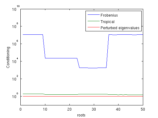
Figure 1: Conditioning of the eigenvalues of different linearizations of a degree $50$ scalar polynomial with random unbalanced coefficients.

Then we build our linearization by means of the function seccomp(b,p) that takes a vector b together with the coefficients of the polynomial and generates the linearization $A(x)$ where $B_{i}(x)=x-\beta_{i}$ for $\beta_{i}={\tt b(i)}$. Finally, we measure the conditioning of the eigenvalues of $A(x)$ by means of the Matlab function condeig.

We have considered three different linearizations:

• The Frobenius linearization obtained by compan(p);

• the secular linearization obtained by taking as $\beta_{i}$ some perturbed values of the roots; these values have been obtained by multiplying the roots by $(1+\epsilon)$ with $\epsilon$ chosen randomly with Gaussian distribution $\epsilon\sim 10^{-12}\cdot N(0,1)$.

• the secular linearization with nodes given by the tropical roots of the polynomial multiplied by unit complex numbers.

The results are displayed in Figure 1. One can see that in the first case the condition numbers of the eigenvalues are much different from each other and can be as large as $10^{8}$ for the worst conditioned eigenvalue. In the second case the condition number of all the eigenvalues is close to $1$, while in the third linearization the condition numbers are much smaller than those of the Frobenius linearization and have an almost uniform distribution.

These experimental results are a direct verification of a conditioning result of [9, Sect. 5.2] that is at the basis of the secsolve algorithm presented in that paper. These tests are implemented in the function files Example1.m and Experiment1.m included in the MATLAB source code for the experiments. A similar behavior of the conditioning for the eigenvalue problem holds in the matrix case.

6.2 The matrix case

Consider now a matrix polynomial $P(x)=\sum_{i=0}^{n}P_{i}x^{i}$. As in the previous case, we start by considering monic matrix polynomials. As a first example, consider the case where the coefficients $P_{i}$ have unbalanced norms. Here is the Matlab code that we have used to generate this test:

⬇

n = 5; m = 64;

P = {};

for i = 1 : n

P{i} = exp(12 * randn) * randn(m);

end

P{n+1} = eye(m);

We can give reasonable estimates to the modulus of the eigenvalues using the Pellet theorem or the tropical roots. See [16, 27], for some insight on these tools.

The same examples given in the scalar case have been replicated for matrix polynomials relying on the Matlab script published on the website reported above by issuing the following commands:

⬇

>> P = Example2();

>> Experiment2(P);

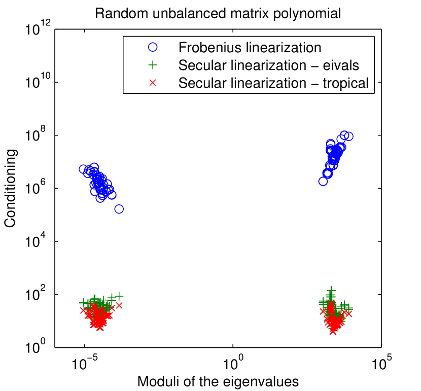
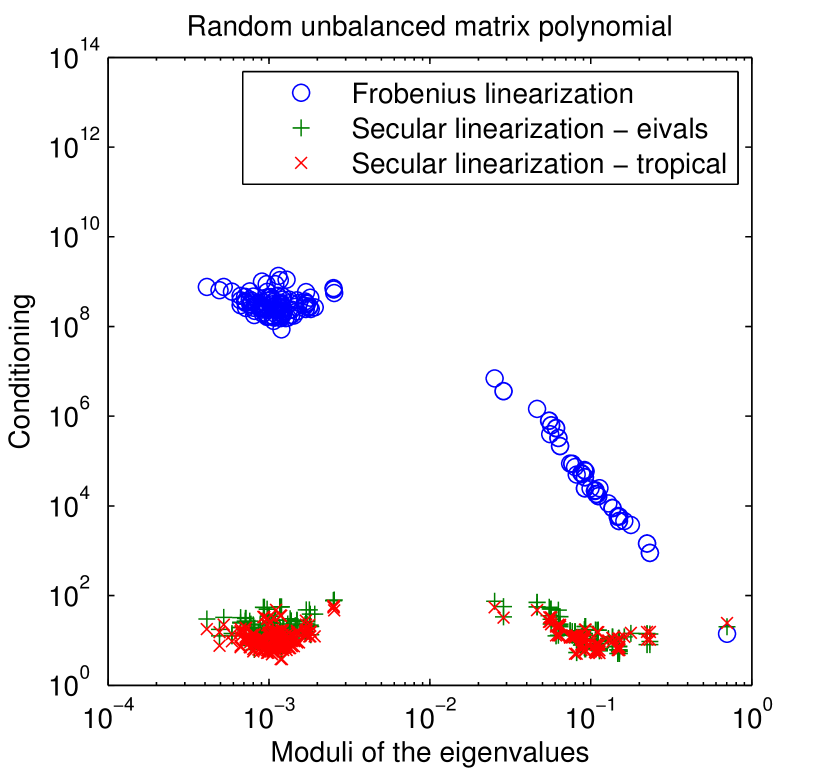
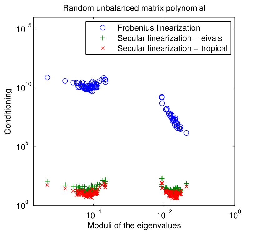
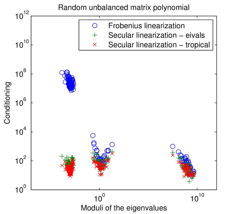
Figure 2: Conditioning of the eigenvalues of different linearizations for some matrix polynomials with random coefficients having unbalanced norms.

We have considered three linearizations: the standard Frobenius companion linearization, and two versions of our secular linearizations. In the first version the nodes $\beta_{i}$ are the mean of the moduli of set of eigenvalues with close moduli multiplied by unitary complex numbers. In the second, the values of $\beta_{i}$ are obtained by the Pellet estimates delivered by the tropical roots.

In Figure 2 we report the conditioning of the eigenvalues, measured with Matlab’s condeig.

It is interesting to note that the conditioning of the secular linearization is, in every case, not exceeding $10^{3}$. Moreover it can be observed that no improvement is obtained on the conditioning of the eigenvalues that are already well-conditioned. In contrast, there is a clear improvement on the ill-conditioned ones. In this particular case, this class of linearizations seems to give an almost uniform bound to the condition number of all the eigenvalues.

Further examples come from the NLEVP collection of [3]. We have selected some problems that exhibit bad conditioning.

As a first example we consider the problem orr_sommerfeld. Using the tropical roots we can find some values inside the unique annulus that is identified by the Pellet theorem. In this example the values obtained only give a partial picture of the eigenvalues distribution. The Pellet theorem gives about 1.65e-4 and 5.34 as lower and upper bound to the moduli of the eigenvalues, but the tropical roots are rather small and near to the lower bound. More precisely, the tropical roots are 1.4e-3 and 1.7e-4 with multiplicities $3$ and $1$, respectively.

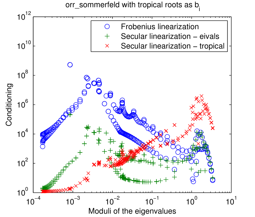
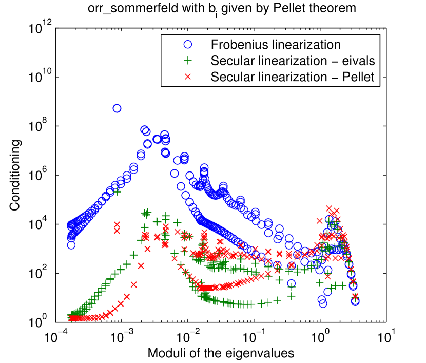
Figure 3: On the left we report the conditioning of the Frobenius and of the secular linearization with the choices of $b_{i}$ as mean of subsets of eigenvalues with close moduli and as the estimates given by the tropical roots. On the right the tropical roots are coupled with estimates given by the Pellet theorem.

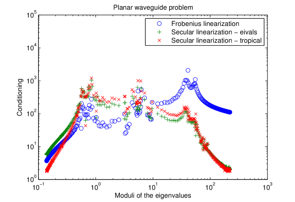
Figure 4: Conditioning of the eigenvalues for three different linearizations on the planar_waveguide problem.

This leads to a linearization $A(x)$ that is well-conditioned for the smaller eigenvalues but with a higher conditioning on the eigenvalues of bigger modulus as can be seen in Figure 3 on the left (the eigenvalues are ordered in nonincreasing order with respect to their modulus). It can be seen, though, that coupling the tropical roots with the standard Pellet theorem and altering the $b_{i}$ by adding a value slightly smaller than the upper bound (in this example we have chosen $5$ but the result is not very sensitive to this choice) leads to a much better result that is reported in Figure 3 on the right. In the right figure we have used b = [ 1.7e-4, 1.4e-3, -1.4e-3, 5 ]. This seems to justify that there exists a link between the quality of the approximations obtained through the tropical roots and the conditioning properties of the secular linearization.

We analyzed another example problem from the NLEVP collection that is called planar_waveguide. The results are shown in Figure 4. This problem is a PEP of degree $4$ with two tropical roots approximately equal to $127.9$ and $1.24$. Again, it can be seen that for the eigenvalues of smaller modulus (that will be near the tropical root $1.24$) the Frobenius linearization and the secular one behave in the same way, whilst for the bigger ones the secular linearization has some advantage in the conditioning. This may be justified by the fact that the Frobenius linearization is similar to a secular linearization on the roots of the unity.

Note that in this case the information obtained by the tropical roots seems more accurate than in the orr_sommerfeld case, so the secular linearization built using the tropical roots and the one built using the block-mean of the eigenvalues behave approximately in the same way.

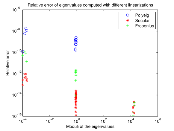
Figure 5: The accuracy of the computed eigenvalues using polyeig, the Frobenius linearization and the secular linearization with the $b_{i}$ obtained through the computation of the tropical roots.

As a last example, we have tried to find the eigenvalues of a matrix polynomial defined by integer coefficients. We have used polyeig and our secular linearization (using the tropical roots as $b_{i}$) and the QZ method. We have chosen the polynomial $P(x)=P_{11}x^{11}+P_{9}x^{9}+P_{2}x^{2}+P_{0}$ where

$$P_{11}=\begin{bmatrix}1&1&1&1\\ &1&1&1\\ &&1&1\\ &&&1\\ \end{bmatrix},\leavevmode\nobreak\ P_{9}=10^{8}\begin{bmatrix}3&1\\ 1&3&1\\ &1&3&1\\ &&1&3\\ \end{bmatrix},P_{2}=10^{8}P_{11}^{t},\leavevmode\nobreak\ P_{0}=\begin{bmatrix}1\\ &2\\ &&3\\ &&&4\\ \end{bmatrix}.$$

In this case the tropical roots are good estimates of the blocks of eigenvalues of the matrix polynomial. We obtain the tropical roots $1.2664\cdot 10^{4}$, $0.9347$ and $1.1786\cdot 10^{-4}$ with multiplicities $2$, $7$ and $2$, respectively. We have computed the eigenvalues with a higher precision and we have compared them with the results of polyeig and of eig applied to the secular linearization and to the standard Frobenius linearization. Here, the secular linearization has been computed with the standard floating point arithmetic. As shown in Figure 5 we have achieved much better accuracy with the latter choice. The secular linearization has achieved a relative error of the order of the machine precision on all the eigenvalues except the smaller block (with modulus about $10^{-4}$). In that case the relative error is about $10^{-12}$ but the absolute error is, again, of the order of the machine precision. Moreover, polyeig fails to detect the eigenvalues with bigger modules, and marks them as eigenvalues at infinity. This can be noted by the fact that the circles relative to the bigger eigenvalues are missing in polyeig plot of Figure 5.

References

- [1] Maha Al-Ammari and Françoise Tisseur. Standard triples of structured matrix polynomials. Linear Algebra Appl., 437(3):817–834, 2012.
- [2] Amir Amiraslani, Robert M. Corless, and Peter Lancaster. Linearization of matrix polynomials expressed in polynomial bases. IMA J. Numer. Anal., 29(1):141–157, 2009.
- [3] Timo Betcke, Nicholas J. Higham, Volker Mehrmann, Christian Schröder, and Françoise Tisseur. NLEVP: A collection of nonlinear eigenvalue problems. http://www.mims.manchester.ac.uk/research/numerical-analysis/nlevp.html.
- [4] Dario A. Bini, Guy Latouche, and Beatrice Meini. Numerical methods for structured Markov chains. Numerical Mathematics and Scientific Computation. Oxford University Press, New York, 2005. Oxford Science Publications.
- [5] Dario A. Bini and Vanni Noferini. Solving polynomial eigenvalue problems by means of the Ehrlich-Aberth method. Linear Algebra and its Applications, 439(4):1130–1149, 2013.
- [6] Dario A. Bini, Vanni Noferini, and Meisam Sharify. Locating the eigenvalues of matrix polynomials. SIAM J. Matrix Anal. Appl., 34(4):1708–1727, 2013.
- [7] Dario A. Bini and Victor Y. Pan. Polynomial and matrix computations. Vol. 1. Progress in Theoretical Computer Science. Birkhäuser Boston, Inc., Boston, MA, 1994. Fundamental algorithms.
- [8] Dario A. Bini and Leonardo Robol. Quasiseparable Hessenberg reduction of real diagonal plus low rank matrices and applications. Submitted.
- [9] Dario A. Bini and Leonardo Robol. Solving secular and polynomial equations: A multiprecision algorithm. Journal of Computational and Applied Mathematics, 272:276–292, 2014.
- [10] Robert M. Corless. Generalized companion matrices in the Lagrange basis. In L. Gonzalez-Vega and T. Recio, editors, Proceedings EACA, June 2004.
- [11] Robert M. Corless and Stephen M. Watt. Bernstein bases are optimal, but, sometimes, Lagrange bases are better. In Proceedings of SYNASC, Timisoara, pages 141–153, 2004.
- [12] Fernando De Terán, Froilán M. Dopico, and D. Steven Mackey. Linearizations of singular matrix polynomials and the recovery of minimal indices. Electron. J. Linear Algebra, 18:371–402, 2009.
- [13] Fernando De Terán, Froilán M. Dopico, and D. Steven Mackey. Fiedler companion linearizations and the recovery of minimal indices. SIAM J. Matrix Anal. Appl., 31(4):2181–2204, 2009/10.
- [14] Fernando De Terán, Froilán M. Dopico, and D. Steven Mackey. Fiedler companion linearizations for rectangular matrix polynomials. Linear Algebra Appl., 437(3):957–991, 2012.
- [15] Fernando De Terán, Froilán M. Dopico, and D. Steven Mackey. Spectral equivalence of matrix polynomials and the index sum theorem. Technical report, MIMS E-Prints, Manchester, 2013.
- [16] Stéphane Gaubert and Meisam Sharify. Tropical scaling of polynomial matrices. In Positive systems, volume 389 of Lecture Notes in Control and Inform. Sci., pages 291–303. Springer, Berlin, 2009.
- [17] Israel Gohberg, Peter Lancaster, and Leiba Rodman. Matrix polynomials. Academic Press, Inc. [Harcourt Brace Jovanovich, Publishers], New York-London, 1982. Computer Science and Applied Mathematics.
- [18] Gene H. Golub. Some modified matrix eigenvalue problems. SIAM Review, 15(2):318–334, 1973.
- [19] Nicholas J. Higham, D. Steven Mackey, Niloufer Mackey, and Françoise Tisseur. Symmetric linearizations for matrix polynomials. SIAM J. Matrix Anal. Appl., 29(1):143–159 (electronic), 2006/07.
- [20] Nicholas J. Higham, D. Steven Mackey, and Françoise Tisseur. The conditioning of linearizations of matrix polynomials. SIAM J. Matrix Anal. Appl., 28(4):1005–1028, 2006.
- [21] Nicholas J. Higham, D. Steven Mackey, and Françoise Tisseur. Definite matrix polynomials and their linearization by definite pencils. SIAM J. Matrix Anal. Appl., 31(2):478–502, 2009.
- [22] Guy Latouche and Vaidyanathan Ramaswami. Introduction to Matrix Geometric Methods in Stochastic Modeling. ASA-SIAM Series on Statistics and Applied Probability. SIAM, Philadelphia, 1999.
- [23] D. Steven Mackey, Niloufer Mackey, Christian Mehl, and Volker Mehrmann. Structured polynomial eigenvalue problems: good vibrations from good linearizations. SIAM J. Matrix Anal. Appl., 28(4):1029–1051 (electronic), 2006.
- [24] D. Steven Mackey, Niloufer Mackey, Christian Mehl, and Volker Mehrmann. Vector spaces of linearizations for matrix polynomials. SIAM J. Matrix Anal. Appl., 28(4):971–1004 (electronic), 2006.
- [25] Marcel F. Neuts. Structured stochastic matrices of type and their applications, volume 5 of Probability: Pure and Applied. Marcel Dekker, Inc., New York, 1989.
- [26] Marcel F. Neuts. Matrix-geometric solutions in stochastic models. Dover Publications, Inc., New York, 1994. An algorithmic approach, Corrected reprint of the 1981 original.
- [27] A.E. Pellet. Sur un mode de séparation des racines des équations et la formule de Lagrange. Bull. Sci. Math., 5:393–395, 1881.
- [28] Vaidyanathan Ramaswami. The generality of Quasi Birth-and-Death processes. In S. Chakravarthy A. Alfa, editor, Advances in Matrix Analytic Methods for Stochastic Models, pages 93–113, 1998.
- [29] Brian T. Smith. Error bounds for zeros of a polynomial based upon Gershgorin’s theorems. J. Assoc. Comput. Mach., 17:661–674, 1970.
- [30] Leo Taslaman, Françoise Tisseur, and Ion Zaballa. Triangularizing matrix polynomials. Linear Algebra Appl., 439(7):1679–1699, 2013.
- [31] Françoise Tisseur. Backward error and condition of polynomial eigenvalue problems. Linear Algebra and its Applications, 309(1):339–361, 2000.
- [32] Françoise Tisseur and Karl Meerbergen. The quadratic eigenvalue problem. SIAM Rev., 43(2):235–286, 2001.
- [33] Françoise Tisseur and Ion Zaballa. Triangularizing quadratic matrix polynomials. SIAM J. Matrix Anal. Appl., 34(2):312–337, 2013.