Rotation in an exact hydro model

Abstract

We study an exact and extended solution of the fluid dynamical model of heavy ion reactions, and estimate the rate of slowing down of the rotation due to the longitudinal and transverse expansion of the system. The initial state parameters of the model are set on the basis of a realistic 3+1D fluid dynamical calculation at TeV energies, where the rotation is enhanced by the build up of the Kelvin Helmholtz Instability in the flow.

I Introduction

In peripheral heavy ion collisions the system has angular momentum. It has been shown in hydrodynamical computations that this leads to a large shear and vorticity CMW13 . Furthermore when the Quark-Gluon Plasma (QGP) is formed with low viscosity CKM , interesting new phenomena may occur like rotation hydro1 , or turbulence, which shows up in form of a starting Kelvin-Helmholtz Instability (KHI) hydro2 ; WNC13 .

Surprisingly, the effects arising from non-vanishing initial angular momentum in fireball hydrodynamics can be studied with the help of exact and explicit, analytic solutions of the equations of hydrodynamics. The pioneers to the application of the hydrodynamical method to high energy particle and nuclear collisions initially neglected the effects from the non-vanishing angular momentum: Belenkij and Landau considered the 1+1 dimensional explosion of a non-expanding region of very high energy density Belenkij:1956cd , while Hwa and Bjorken considered  Hwa:1974gn ; Bjorken:1982qr a boost-invariant, already asymptotic expansion as the initial condition of 1+1 dimensional expansion governed by relativistic hydrodynamics.

However, if the collision of two protons or two heavy ions is not exactly head-on, there is a non-vanishing initial angular momentum present in the initial conditions, which was for a long time neglected. However, rather recently, numerical investigations of relativistic hydrodynamics CMW13 ; CKM ; hydro1 ; hydro2 ; WNC13 , as well as exact and explicit analytic solutions of relativistic and non-relativistic hydrodynamics were found for rotating fluids  Nagy:2009eq ; Csorgo:2013ksa . It took 35 years after the publication of the first exact, non-rotational solution in a similar class Bondorf:1978kz to find and publish rotating solutions of hydrodynamics, a long road with lots of surprises and unexpected turns, that were recently briefly summarized in ref.  Csorgo:2013ksa . In ref. McI-Teo the AdS/CFT holography method is used to study the QGP created in heavy ion collisions. The authors chose two types of velocity profiles, which do not favor instability classically, and they use the planar black hole geometry to compute the fluid shear by using parameters predicted in hydro2 . The discussion shows that for the two clasically stable configurations in the holographic model instability develops very slowly for lower chemical potentials, but turbulence may still exist for high chemical potentials. Finding of these rotating solutions started to shed more light on the effects of rotation, which plays a very important role McI2014 in shaping the events in astrophysical, hydrodynamically evolving systems, turbulence, or in eddy and vortex formation in fluid dynamics. This motivates the subject of the present paper, which evaluates numerically some of the important characteristics of the fireball (like the size of the fireball along the axis of rotation and the size of the fireball in the plane perpendicular to the rotation) for quasi-realistic initial conditions and compares it with the case when the initial angular momentum is negligible, or is neglected.

Based on ref. hydro2 we can extract some basic parameters of the rotation obtained with numerical fluid dynamical model PICR. These parameters are extracted from model calculation of a Pb+Pb collisions at $\sqrt{s_{NN}}=2.76$ A TeV and at the impact parameter of $b=0.7b_{max}$, with high resolution and thus small numerical viscosity. Thus, in this collision the KHI occurs and enhances rotation at intermediate times, because the turbulent rotation gains energy from the original shear flow. The turbulent rotations leads to a rotation profile where the rotation of the external regions lags behind the rotation of the internal zones. This is a typical growth of the KHI. See Table 1.

${}^{|}_{|}$ $t$	$Y$	$\dot{Y}$	$\theta$	$R$	$\dot{R}$	$\omega$
(fm/c)	(fm)	(c)	(Rad)	(fm)	(c)	(c/fm)
0.	4.38	0.90	0.000	3.68	0.60	0.0175
2.	6.18	0.88	0.035	4.87	0.84	0.0350
4.	7.91	0.84	0.105	6.56	0.97	0.0520
6.	9.54	0.80	0.209	8.49	0.86	0.0700
8.	11.09	0.76	0.349	10.21	0.81	0.0350

Table 1: Time dependence of some characteristic parameters of the fluid dynamical calculation presented in ref. hydro2 . $R$ is the average transverse radius ($R\approx\sqrt{XZ}$), $Y$ is the length of the system in the direction of the axis of the rotation $y$, $\theta$ is the polar angle of the rotation of the interior region of the system measured versus the $z$ directed, beam axis, of the reaction plane, $[x,z]$ plane, $\dot{R},\ \dot{Y}$ are the speeds of expansion in radial and rotational axis directions, and $\omega$ is the angular velocity of the internal region of the matter during the collision.

The initial angular momentum of the system is large, $L_{y}=-1.05\times 10^{4}\hbar$ in mid-peripheral collision. This is arising from the pre-collision state. In refs. CMW13 ; hydro1 ; hydro2 the same Initial State (IS) model is used, before the PICR fluid dynamical model started. The IS model M1 ; M2 describes the first 4 fm/c time period after the moment when the Lorentz contracted, thin projectile and target slabs (like in the CGC model) penetrate each other. The matter is then divided into longitudinally ($z$ directed) expanding (fire)streaks. The $[x,y]$ transverse plane is divided into surface elements according to the resolution of the PICR model, and each element belongs to one streak. The streak expansion is described in a one-dimensional classical Yang-Mills field, spanned by the color charges at the two ends of the streak. This field slows down the expansion due to the large string-rope tension. The IS dynamics satisfies the momentum conservation $Streak\ by\ Streak$, and this way the total angular momentum of the IS is also exactly conserved. During the IS model the dynamics is one dimensional ($z$), with $z$ directed velocities only, but the expansion is different in different transverse points.

After 4 fm/c of the IS model, local equilibrium is reached and the PICR (3+1)D fluid dynamical model starts (with $t=0$ fm/c fluid dynamical model time). Then, due to the fluid dynamical development and equilibration, the $x$-directed velocity starts to increase and the average of the $z$-directed velocity decreases. This way the angular momentum is exactly conserved in the (3+1)D fluid dynamical calculation. Thus the $x$-directed velocity or otherwise the rotation in the horizontal plane starts up delayed. This is a fully realistic model of the initial longitudinally transparent non-equilibrium dynamics, and the subsequent equilibration of rotation on a larger scale hydro2 .

As the initial conditions and initial times in the exact model and in the PICR (3+1)D model are not identical we have matched the time coordinates such that $t_{exact}=0$ fm/c in the exact model corresponds to: $t=3$ fm/c in the full (3+1)D calculation.

If we compare the rotation of the horizontal plane ($x$ directed velocity) only, then the PICR model and the exact model are becoming similar at $t=6$ ($t_{exact}=3$) fm/c and after (see Table I and Table II). If however, we estimate the average of the $z$ directed velocity also, and consider then the average of the $x$ and $z$ directed velocities, the two models are becoming similar already at $t=4$ ($t_{exact}=1$) fm/c and after. Thus, the applicability of the exact model with the parameters chosen here, starts approximately after $t=5$ fm/c on the timescale of the PICR model. The radius, $R$, parameters are matched to each other in the two models s0 that in the (3+1)D model at the same time moments, $t=5$ and $8$ fm/c the radii are 8.49 and 10.21 fm for a sharp matter surface, while in the exact model the corresponding radii are 3.97 and 5.36 fm respectively (i.e. about half of the previous values) but these represent the width parameter of an infinite Gaussian matter distribution.

The initial part of the (3+1)D model describes the equilibration of the rotational flow from the initial shear flow, which rotation then leads to a maximal, azimuthally averaged angular velocity. Then the system expands and the angular velocity decreases. The exact model, assuming uniform rotation can only describe this second phase of the process. It is important to mention that the KHI facilitates the equilibration and speed up of the rotation and leads to an earlier and bigger maximal angular velocity. In this case the applicability of the exact model is more extended in time, and spans the range between the equilibration of the rotation and the freeze out. At lower beam energies and small impact parameters (i.e. at lover angular momentum) the timespan of the applicability of exact model should be tested separately.

We want to use these fluid dynamical calculations to test a new family of exact rotating solutions Csorgo:2013ksa , which may provide more fundamental insight to the interaction between the rotation and expansion of the system. This model offers a few possible variations, here we chose the version 1A to test. We change the axis labeling of ref. Csorgo:2013ksa , so that the axis of the rotation is $y$ while the transverse plane of the rotation is the $[x,z]$ plane. Thus the values extracted from the results of the fluid dynamical model, hydro2 , should take this into account. The initial radius parameter, $R$, corresponds to the system size in the $x$ or $z$ directions in hydro, and we assume an $x,z$ symmetry in the exact model. The rotation axis is the $y$ axis in hydro and now also in the exact model. The exact model assumes azimuthal symmetry, so it cannot describe the beam directed elongation of the system, but this is arising from the initial beam momentum, and we intend to describe the rotation of the interior part of the reaction plane and the rotation there.

In Section II we recapitulate some of the central results of ref. Csorgo:2013ksa for clarity and so that the manuscript be self-contained. New studies will start in Section III.

II From the Euler Equation to Scaling

In ref. Csorgo:2013ksa it is assumed that the temperature and the density have time independent distributions with respect to a scaling variable: $s=r_{x}^{2}/X^{2}+r_{y}^{2}/Y^{2}+r_{z}^{2}/Z^{2}\ .$ Now instead we assume azimuthal symmetry and thus use the corresponding cylindrical coordinates instead of $(x,y,z)$. However, we also use the coordinates in length dimension, $(r_{\rho},r_{\varphi},r_{y})$, so that

$$r_{\rho}=\rho,\ \ r_{\varphi}=r_{\rho}\varphi,\ \ r_{y}=y\ .$$

These represent the so called ”out, side, long” directions. The boundary values of these coordinates are then $(R,S,Y)$. The scaling variables can be introduced as

$$s_{\rho}=r_{\rho}^{2}/R^{2},\ \ s_{\varphi}=r_{\varphi}^{2}/S^{2}\ \ s_{y}=r_{y}^{2}/Y^{2}\ ,$$

where $S$ is the roll-length on the outside circumference, starting from $\varphi_{0}=0$ and $S_{0}=0$ at $t_{0}$,   $S=R\varphi$ and $\dot{\varphi}~{}=~{}\omega$ and this displacement is orthogonal to the longitudinal and transverse displacements. The internal roll-length is $r_{\varphi}=\varphi\,r_{\rho}$, the corresponding velocity is $v_{\varphi}=\omega\,r_{\rho}$, and so $v_{\varphi}^{2}=\omega^{2}\,r_{\rho}^{2}$. On the other hand from the scaling of $r_{\rho}$, it follows that $r_{\rho}^{2}=R^{2}\,s_{\rho}$.

Nevertheless, in case of these scaling variables the distributions of density and temperature, $n(s)$ and $T(t,s)$ should not depend on $s_{\varphi}$ or $r_{\varphi}$, just on the radius and the longitudinal coordinates. Therefore in this work we introduce another scaling variable:

$$s\equiv s_{\rho}+s_{y}\ .$$

Our reference frame is then spanned by the directions $(r_{\rho},r_{\varphi},r_{y})$. In this case due to the azimuthal symmetry the derivatives, $\partial s/\partial r_{\varphi}$ vanish. In this coordinate system the volume is $V=2\pi R^{2}Y$.

The derivatives, $\dot{R}(t_{0})$ and $\dot{Y}(t_{0})$ in this exact model should not equal the ones obtained from the fluid dynamical model, because in the more realistic model the density and velocity profiles do not agree with the exact model’s assumptions. Also initially in the realistic fluid dynamical model the angular momentum increases in the central region due to the developing turbulence, while in the exact model it is monotonously decreasing due to the scaling expansion.

For simplicity we also assume that the Equation of State (EoS), $\epsilon=\epsilon(n,p)$, with a constant $\kappa$ is:

$$\epsilon=\kappa p\ \ \ {\rm and}\ \ \ p=nT\ ,$$ (1)

where $n$ is the conserved net baryon charge and $T$ is the temperature.

Now we calculate the eq. (15) in ref. Csorgo:2013ksa .

$$n\,m\,(\partial_{t}+\mbox{\boldmath$v$}\cdot\nabla)\mbox{\boldmath$v$}=-\nabla p\ .$$ (2)

For the variables of this equation we have:

$$T = T_{0}\left(\frac{V_{0}}{V}\right)^{1/\kappa}\mathcal{T}(s)\ ,$$

$$n = n_{0}\frac{V_{0}}{V}\nu(s),$$

$$\nu(s) = \frac{1}{\mathcal{T}(s)}e^{-\frac{1}{2}\int_{0}^{s}\frac{du}{\mathcal{T}(u)}},$$ (3)

and in addition in ref. Csorgo:2013ksa it is assumed that the temperature and the density have time independent distributions with respect to the scaling variable $s$.

Thus, for the right hand side of eq. (2):

$$-\nabla p = -\nabla nT$$ (4)

$$= -n_{0}\frac{V_{0}}{V}T_{0}\left(\frac{V_{0}}{V}\right)^{1/\kappa}\nabla e^{-\frac{1}{2}\int_{0}^{s}\frac{du}{\mathcal{T}(u)}}$$

$$= -n_{0}\frac{V_{0}}{V}T_{0}\left(\frac{V_{0}}{V}\right)^{1/\kappa}e^{-\frac{1}{2}\int_{0}^{s}\frac{du}{\mathcal{T}(u)}}(-\frac{1}{2})\frac{1}{\mathcal{T}(s)}\nabla s$$

$$= nmQ/V^{\gamma}\left(\frac{r_{\rho}}{R^{2}}\mbox{\boldmath$e$}_{\rho}{+}\frac{r_{y}}{Y^{2}}\mbox{\boldmath$e$}_{y}\right)\ ,$$

where $\gamma=1/\kappa$ and $Q\equiv\frac{T_{0}V_{0}^{\gamma}}{m}$.

Using the $\rho,\varphi,y$ coordinates, the rotation would show up as an independent orthogonal term. However, the closed system has no external torque, and the internal force from the gradient of the pressure is radial, which does not contribute to tangential acceleration. The change of the angular velocity arises from the angular momentum conservation in the closed system as a constraint, so we do not have to derive additional dynamical equations to describe the evolution of the rotation.

Now for the left hand side of eq. (2), the velocity, $\mbox{\boldmath$v$}=\mbox{\boldmath$v$}(t,r_{\rho},r_{\varphi},r_{y})$, scales as

$$\mbox{\boldmath$v$}=v_{\rho}\mbox{\boldmath$e$}_{\rho}{-}v_{\varphi}\mbox{\boldmath$e$}_{\varphi}{+}v_{y}\mbox{\boldmath$e$}_{y}=\frac{\dot{R}}{R}r_{\rho}\mbox{\boldmath$e$}_{\rho}{-}\omega r_{\rho}\mbox{\boldmath$e$}_{\varphi}{+}\frac{\dot{Y}}{Y}r_{y}\mbox{\boldmath$e$}_{y}\ .$$ (5)

Let us first calculate the time derivatives for the components. (See e.g. Stoecker_handbook ):

$$\partial_{t}v_{\rho} = \left[\left(\frac{\ddot{R}}{R}{-}\frac{\dot{R}^{2}}{R^{2}}\right)-\omega^{2}\right]r_{\rho},$$

$$\partial_{t}v_{\varphi} = -\omega\frac{\dot{R}}{R}r_{\rho},\ \ \ \partial_{t}v_{y}=\left[\frac{\ddot{Y}}{Y}{-}\frac{\dot{Y}^{2}}{Y^{2}}\right]r_{y}.$$ (6)

The other term of the comoving derivative gives:

$$(\mbox{\boldmath$v$}\cdot\nabla)\mbox{\boldmath$v$}=\frac{\dot{R}^{2}}{R^{2}}r_{\rho}\mbox{\boldmath$e$}_{\rho}+\omega\frac{\dot{R}}{R}r_{\rho}\mbox{\boldmath$e$}_{\varphi}+\frac{\dot{Y}^{2}}{Y^{2}}r_{z}\mbox{\boldmath$e$}_{z}\ .$$ (7)

Adding eq. (6) and (7) we get:

$$mn(\partial_{t}{+}\mbox{\boldmath$v$}\cdot\nabla)v_{\rho} = mn\left[\left(\ddot{R}/R\right)-\omega^{2}\right]r_{\rho}\ ,$$

$$mn(\partial_{t}{+}\mbox{\boldmath$v$}\cdot\nabla)v_{z} = mn\left(\ddot{Y}/Y\right)r_{z}\ .$$ (8)

Then the equality of the right hand side and left hand side of the Euler equation (2) leads to the ordinary differential equations. Multiplying the two non-vanishing equations with $R^{2}$ and $Y^{2}$ respectively yields:

$$R\ddot{R}-W/R^{2} = Y\ddot{Y}=\frac{T_{0}}{m}\left(\frac{V_{0}}{V}\right)^{\gamma}\ ,$$ (9)

where $W~{}\equiv~{}\omega_{0}^{2}~{}R_{0}^{4}$. Notice that from the angular momentum conservation $\omega=\omega_{0}R_{0}^{2}/R^{2}$, thus the rotational term, $R^{2}\omega^{2}$ in the equation, takes the form $W/R^{2}$.

Notice that due to the EoS the pressure is proportional to the baryon density $n$, just as the r.h.s. of the Euler equation, therefore the equation of motion does not depend on $n$ or $n_{0}$.

III Conservation Laws

If we want to calculate the energy of the whole system, then we should actually integrate it for the whole volume, $V$. Thus, not only the scaling of $\mbox{\boldmath$v$}=(v_{\rho},v_{\varphi},v_{z})$ but the particle density distribution, $n(s)$ will also play a role.

The rotational energy at the surface is $\mathcal{E}_{Side}\equiv\frac{1}{2}m\dot{S}^{2}=\frac{1}{2}mR^{2}\omega^{2}$, and if we express $\omega$ via $\omega_{0}$ using the relation $\omega=\omega_{0}R_{0}^{2}/R^{2}$, then $\mathcal{E}_{Side}=W/R^{2}$, i.e. just as before. The expansion energy at the surface is $\mathcal{E}_{Out}\equiv\frac{1}{2}m\dot{R}^{2}$, and for the longitudinal direction, $\mathcal{E}_{Long}\equiv\frac{1}{2}m\dot{Y}^{2}$.

For the interior we can calculate the radial and longitudinal expansion velocities and the corresponding kinetic energies, as well as the kinetic energy of the rotation. In the evaluation of the internal and kinetic energies the radial and longitudinal density profiles of the system should be taken into account.

We now assume that the temperature profile is flat, and consequently the density profiles are Gaussian and separable ACLS01 . With this approximation the different integrated energies are calculated. The boundary of the spatial integrals can be set to infinity or to finite values ($s_{\rho M},\ s_{yM}$) as well. To be consistent with the earlier exact model results we integrate now to infinity, the integrals are finite.

Adding up the kinetic energies yields

$$E_{K}=\frac{1}{2}mN_{B}\left(\alpha^{2}\dot{R}^{2}+\alpha^{2}R^{2}\omega^{2}+\beta^{2}\dot{Y}^{2}\right)\ ,$$ (10)

where
$\alpha^{2}\!\equiv\!4\sqrt{2}\,C_{n}I_{B}({\small\frac{1}{2}}s_{yM})I_{C}({\small\frac{1}{2}}s_{\rho M})\ {\rm and}\,\\ \beta^{2}\!\equiv\!4\sqrt{2}\,C_{n}I_{A}({\small\frac{1}{2}}s_{\rho M})I_{D}({\small\frac{1}{2}}s_{yM}),{\rm where}\\$ $C_{n}=1\left/\left[2\sqrt{2}\,I_{A}(0.5s_{\rho M})\,I_{B}(0.5s_{yM})\right]\right.$  . Now we extend the boundaries to infinity, thus $\alpha^{2}=2$ and $\beta^{2}=1$.

Here $\alpha^{2}$ and $\beta^{2}$ are time independent, because they depend on the scaling variables only. If we divide this result by the conserved baryon charge, $N_{B}$, we will get

$$\frac{E_{K}}{N_{B}}=\frac{1}{2}m\left[\alpha^{2}\left(\dot{R}^{2}{+}R^{2}\omega^{2}\right)+\beta^{2}\,\dot{Y}^{2}\right]\ .$$ (11)

Based on the EoS, $\epsilon=\kappa p=\kappa nT$, one can calculate the compression energy also based on the density profiles of $n(s)$ and $\epsilon(s)=\kappa\,n(s)T$. Here we made the same simplifying assumptions on the density profiles as before.

Then volume integrated internal energy and net baryon charge will have the same density profile, normalized to $N_{B}$:

$$E_{int} = \kappa\int pdV=\kappa\int nTdV=\kappa N_{B}T_{0}(V_{0}/V)^{\gamma}\,C_{n}$$ (12)

$$\times \frac{1}{V}\ 2\pi R^{2}Y\!\!\int_{0}^{s_{yM}}\!\!\int_{0}^{s_{\rho M}}\!\!\!\nu(s)\ ds_{\rho}\,\frac{ds_{y}}{\sqrt{s_{y}}}$$

$$= \kappa N_{B}T_{0}(V_{0}/V)^{\gamma}\ =\ \kappa T_{0}\left(\frac{V_{0}}{V}\right)^{\gamma}$$

where $C_{n}$ is the normalization constant.

IV Reduction to a Single Differential Equation

Now following the method of ref. ACLS01 , we study the following combination:

$${\cal F} = {\small\frac{1}{2}}\partial_{t}^{2}\left(\alpha^{2}R^{2}+\beta^{2}Y^{2}\right)=\partial_{t}\left(\alpha^{2}R\dot{R}+\beta^{2}Y\dot{Y}\right)$$ (13)

$$= \alpha^{2}\dot{R}^{2}+\beta^{2}\dot{Y}^{2}+\alpha^{2}R\ddot{R}+\beta^{2}Y\ddot{Y}.$$

Here we used the notation $\partial_{t}=\frac{\partial}{\partial t}\ \ {\rm and}\ \ \partial_{t}^{2}=\frac{\partial^{2}}{\partial t^{2}}.$ Now we can replace the last two terms, $\alpha^{2}R\ddot{R},\ \beta^{2}Y\ddot{Y}$, by using eqs. (9), i.e. we use the Euler equation (2). Then we obtain:

$${\cal F}=\alpha^{2}\dot{R}^{2}+\beta^{2}\dot{Y}^{2}+\alpha^{2}\frac{W}{R^{2}}+(\alpha^{2}{+}\beta^{2})\frac{Q}{(2\pi R^{2}Y)^{\gamma}},$$ (14)

On the other hand from the energy conservation, $E_{tot}=E_{k}+E_{int}$, we get that

$$\frac{E_{tot}}{N_{B}\,m}=\frac{1}{2}\left[\alpha^{2}\dot{R}^{2}{+}\beta^{2}\dot{Y}^{2}{+}\alpha^{2}\frac{W}{R^{2}}{+}\frac{2\kappa Q}{(2\pi R^{2}Y)^{\gamma}}\right],$$ (15)

where we used the EoS and thus the parameter $\kappa$ now appears in the expression of the energy.

Now, if our EoS is such that

$$\kappa=(\alpha^{2}{+}\beta^{2})\ /2\ ,$$ (16)

then ${\cal F}=2E_{tot}/(N_{B}\,m)=$ const., and in the same type of calculation as in ref. ACLS01 , we can introduce

$$U^{2}(t)\equiv\alpha^{2}R^{2}(t)+\beta^{2}Y^{2}(t),$$ (17)

which satisfies

$$\partial_{t}^{2}\left(\alpha^{2}R^{2}+\beta^{2}Y^{2}\right)=\partial_{t}^{2}U^{2}(t)=2{\cal F}\ .$$ (18)

Thus, the solution of eq. (18), can be parametrized as:

$$U^{2}(t)=A(t-t_{0})^{2}+B(t-t_{0})+C\ ,$$ (19)

$${\rm where:}\ \ A = \alpha^{2}\dot{R}_{0}^{2}+\beta^{2}\dot{Y}_{0}^{2}+\alpha^{2}W/R_{0}^{2}+(\alpha^{2}{+}\beta^{2})\frac{T_{0}}{m}$$

$$B = 2\alpha^{2}R_{0}\dot{R}_{0}+2\beta^{2}Y_{0}\dot{Y}_{0}\phantom{\frac{T_{0}}{m}}$$

$$C = \alpha^{2}R_{0}^{2}+\beta^{2}Y_{0}^{2}\phantom{\frac{T_{0}}{m}}\ .$$ (20)

${}^{|}_{|}$ $t$	$Y$	$\dot{Y}$	$\theta$	$R$	$\dot{R}$	$\omega$
(fm/c)	(fm)	(c)	(Rad)	(fm)	(c)	(c/fm)
0.0	4.000	0.300	0.000	2.500	0.250	0.150
1.0	4.349	0.393	0.135	2.852	0.441	0.115
2.0	4.776	0.458	0.235	3.360	0.567	0.083
3.0	5.258	0.503	0.307	3.970	0.646	0.059
4.0	5.777	0.534	0.358	4.642	0.696	0.044
5.0	6.322	0.555	0.397	5.356	0.729	0.033
6.0	6.886	0.571	0.426	6.096	0.752	0.025
7.0	7.462	0.582	0.449	6.856	0.767	0.020
8.0	8.049	0.591	0.467	7.629	0.779	0.016

Table 2: Time dependence of characteristic parameters of the exact fluid dynamical model Csorgo:2013ksa . R is the transverse radius, Y is the (rotation axis directed) length of the system, $\dot{R},\ \dot{Y}$ are the speed of expansion in transverse and axis directions, $\theta$ id the angle of rotation, and $\omega$ is the angular velocity of the matter.

Let us take one of the Euler equations from eq. (9),

$$\ddot{Y}=\frac{Q}{Y(2\pi R^{2}Y)^{\gamma}}\ ,$$ (21)

and express $R^{2}$ in terms of $U^{2}(t)$ which is known based on the energy conservation:

$$R^{2}(t)=(U^{2}(t)-\beta^{2}Y^{2})/\alpha^{2}\ .$$ (22)

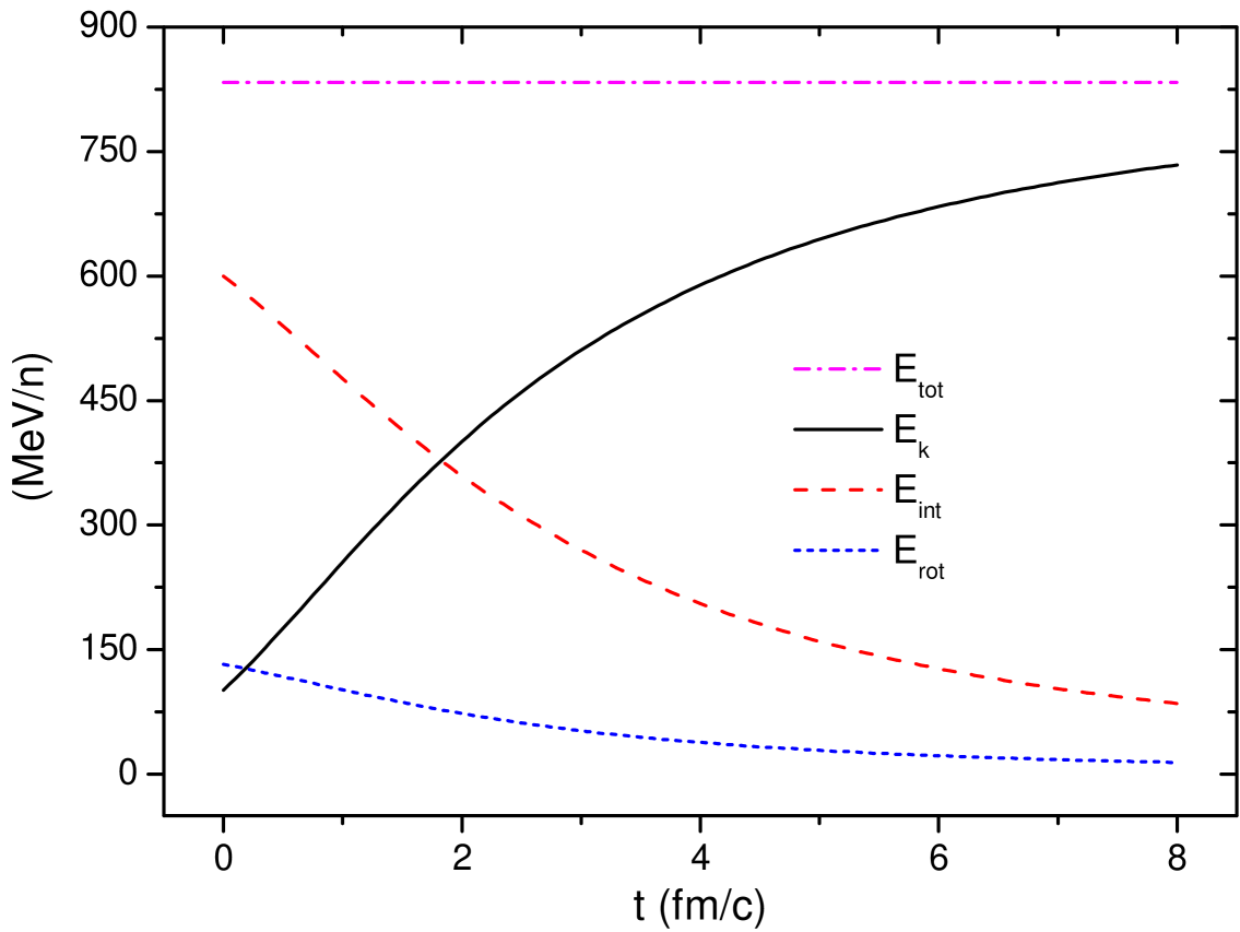
Figure 1: (color online) The time dependence of the kinetic energy of the expansion, $E_{K}$, of the internal energy, $E_{int}$, and the rotational energy, $E_{rot}$ per nucleon in the exact model with the initial conditions described above. The kinetic energy of the expansion is increasing, at the cost of the decreasing internal energy and the slower decreasing rotational energy. The rotational energy is decreasing to the half of the initial one in 2.1 fm/c.

This leads to a 2nd order differential equation for $Y(t)$:

$$\ddot{Y}=\frac{\alpha^{2\gamma}\,Q}{Y\left[2\pi Y(U^{2}(t){-}\beta^{2}Y^{2})\right]^{\gamma}}=f(Y,t)\ ,$$ (23)

which can be solved. Then $R(t)$ and $\dot{R}(t)$ are given by eqs. (22) and (14) respectively.

In the main steps we followed ref. ACLS01 , however it turned out that the modified last step of the method provides a more straightforward solution. We show the model provides an excellent and simple semi-analytic tool to study the effects and consequences of an expanding and rotating system.

We used the Runge Kutta RungeKutta method to solve this differential equation. We need the constants, $Q$ and $W$, as well as the initial conditions for $R$ and $Y$.

Based on fluid dynamical model calculation results, presented in table 1, we chose the parameters: $T_{0}=250\ {\rm MeV},\ m=939.57{\rm MeV}\ \omega_{0}=0.15$ c/fm. For the internal region we take the initial radius parameters as $R_{0}=2.5{\rm fm\ and\ }\dot{R}=0.25{\rm c}$, and we disregard the larger extension in the beam direction, because our model is azimuthally symmetric and because the beam directed large elongation is a consequence of the initial beam directed momentum excess, which is converted into rotation in the course of initial equilibration only. In this exact model the rotation axis, denoted by $Y$, corresponds to the out of plane, $y$ direction in the fluid dynamical model (and not to the beam direction!). Due to the eccentricity at finite impact parameters, with an almond shape profile, the initial out of plane size is larger than the in plane transverse size, so we chose $Y_{0}=4.0{\rm fm\ and\ }\dot{Y}=0.3{\rm c}$.

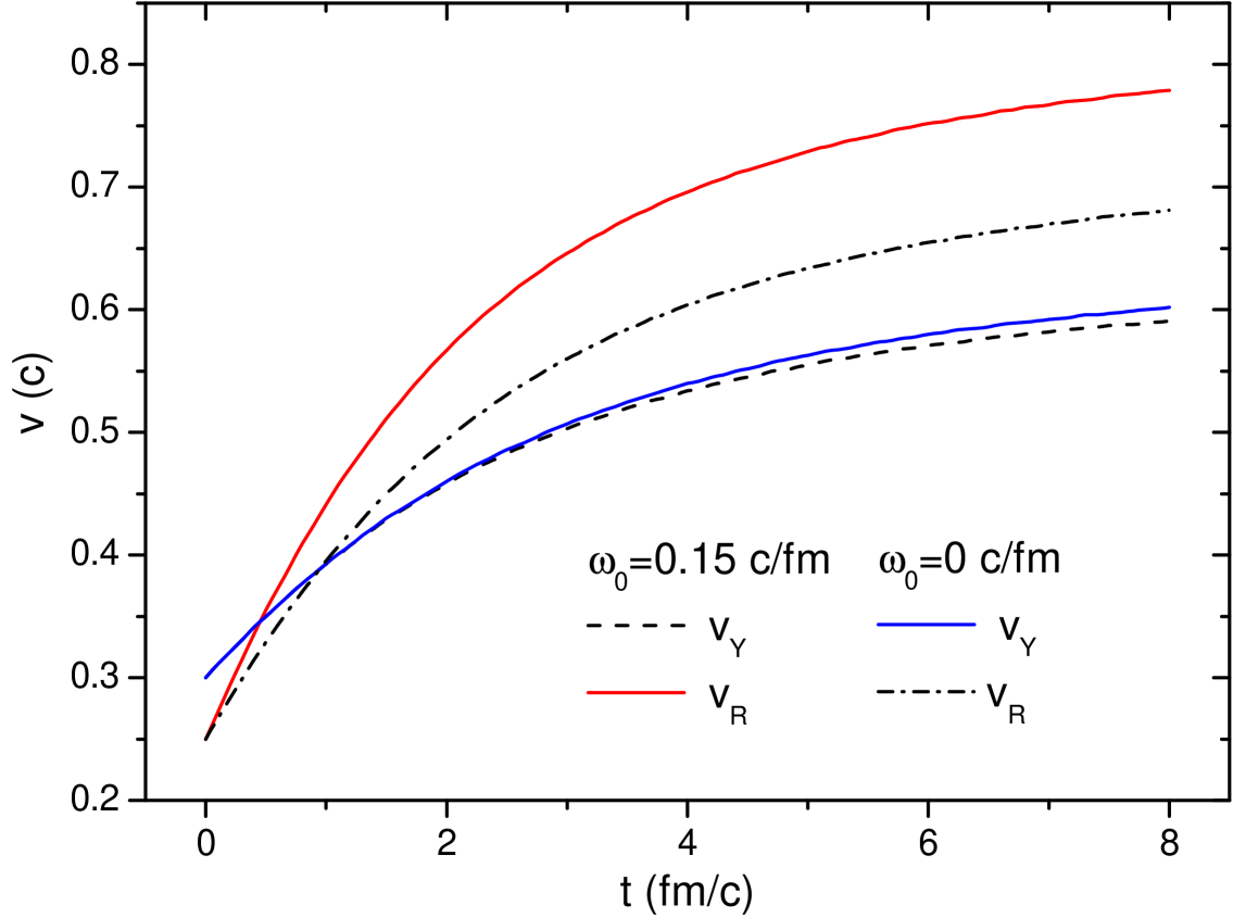
Figure 2: (color online) The time dependence of the velocity of expansion in the transverse radial direction, $v_{R}$ and in the direction of the axis of the rotation, $v_{Y}$.

As the exact solution is able to describe the monotonic expansion, and so the steady decrease of the rotation, we start from a higher initial angular velocity than shown by the fluid dynamical model, PICR, as the angular velocity was measured versus the horizontal plane where the angular velocity starts from zero.

With these initial parameters the exact model yields a dynamical development shown in Table 2. According to expectations the radius, $R$, and the axis directed size, $Y$, are increasing, the angular velocity, $\omega$ decreases, The total energy is conserved, while the kinetic energy of expansion is increasing, and that of the rotation and internal energy are decreasing. See Fig. 1.

The change of the expansion velocity is shown in Fig. 2. The expansion velocity is increasing in both directions. While in the axis, $y$, direction the velocity increases from 0.4 c to 0.5 c in 8 fm/c time, the radial expansion increases faster, in part due to the centrifugal force from the rotation. The radial expansion velocity increases by near to 10 percent due to the rotation, which is significant, while the expansion in the direction of the axis of rotation is hardly changed. In both cases the expansion in the radial direction is large. This is due to the choice of a small initial radius parameter. This exact, perfect fluid model overestimates the radial expansion velocity due to the lack of dissipation and the Freeze out happens earlier than 8 fm/c as at this time the size of the system is already reaching 16 fm (see Fig. 3) larger than the estimates based two particle correlation experiments. At the same time, although the rotation is non-relativistic, the Hubble flow terms are large and the Hubble flows are relativistic. This problem is not new, it is also present in ref. [15] and in earlier exact models. The radial (directional Hubble) solutions go smoothly over to a relativistic exact solution of hydrodynamics CsCsHK03 . As the velocity of rotation decreases faster asymptotically than the Hubble flow, the rotation is not expected to influence essentially the asymptotic relativistic behaviour of the flow.

The more rapid velocity change arises partly from the centrifugal acceleration of the rotation, but also from the fact that the initially smaller transverse size increases faster in the direction of equal sizes in both directions. See Fig. 3.

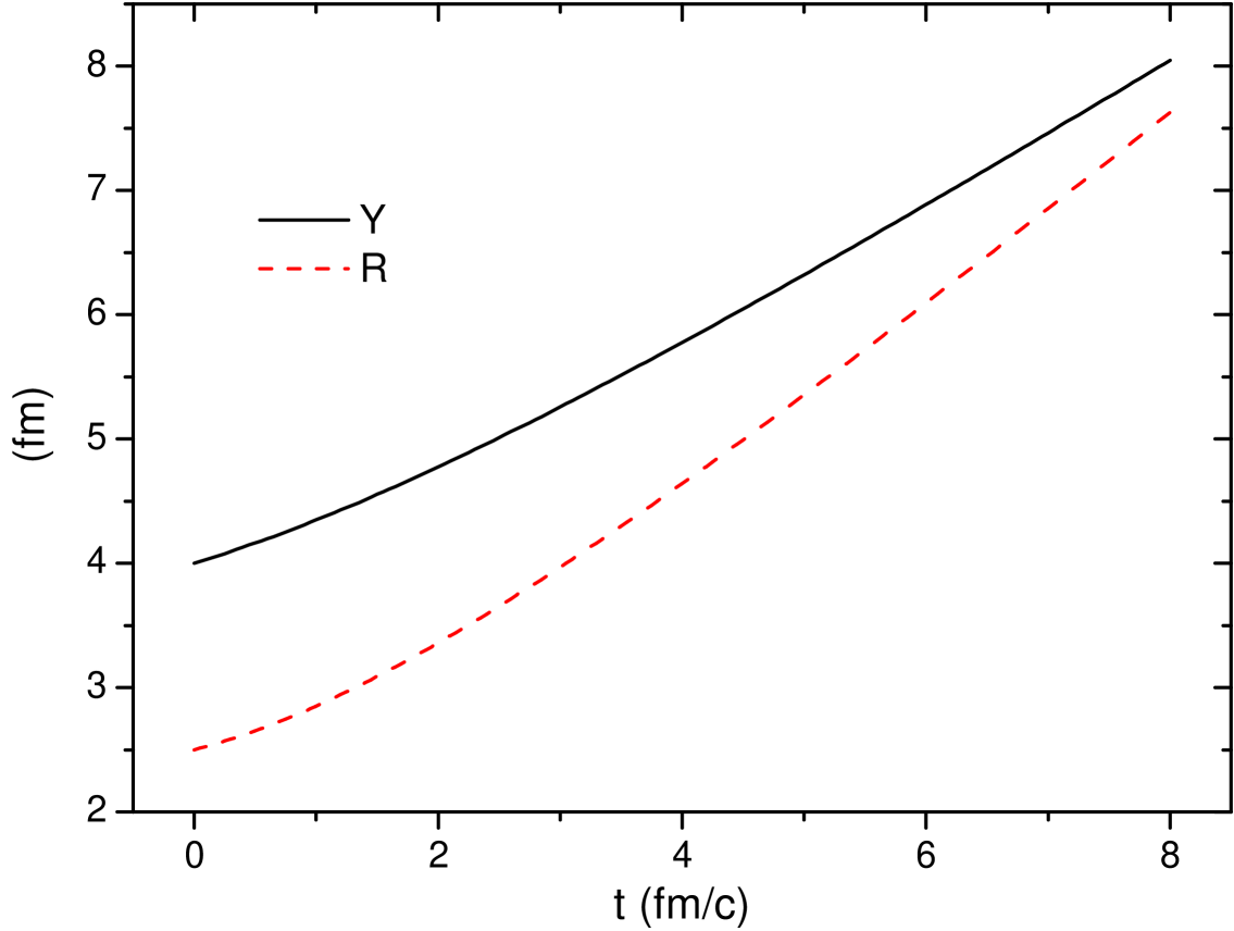
Figure 3: (color online) The time dependence of the Radial, $R$, and the $y$ axis directed size, $Y$, of the expanding system. As the $y$ directed velocity is initially larger and its change is relatively smaller the change of the rate of increase is hardly visible.

V Conclusions

In conclusion, the exact model can be well realized with parameters extracted from detailed, high resolution, 3+1D relativistic fluid dynamical model calculations with the PICR code. The exact model describes a system with with one single, uniform $\omega$ representing the whole matter at a given moment of time. Depending on the impact parameter, the system size, the beam energy, and the transport properties, the uniform flow can develop from the initial shear flow at different times. It is important to know when this time is reached in a collision and with which parameters. Then this will enable us to conclude about the material parameters and the equilibration dynamics. The exact model provides us with a simple and straightforward tool to give a precise estimate about the time moment when the rotation equilibrated and the parameters of the matter at that moment.

The exact model can be used as a tool, when the rotations can be detected at freeze out. Then it provided an estimate of the rate of decrease of angular speed and rotational energy due to the expansion in an explosively expanding system. This indicates that the effects of rotation can be observable in case of rapid freeze out and hadronization, and the rate if conversion from rotational energy to expansion can be studied in detail depending on the parameters of the model.

At the same time these studies also show that the initial rotation is also influencing the rate of decrease of rotation. Here especially the enhancement of initial rotation due to the Kelvin Helmholtz Instability is essential, although this is a special (3+1)D instability, which in itself cannot be included in the exact rotational model. Still the presence of the KHI is essential to generate the rotation, and thus the observation of the rotation is strongly connected to the evolving turbulent instability in low viscosity Quark-gluon plasma.

Due to the difference of the time evolution between the numerical and the exactly solvable hydrodynamical models at early times one expects that the predictions of the two models in the sector of penetrating probes (dilepton spectrum, direct photon spectra, elliptic flow, HBT) will be different and these differences later on can be used to explore the mechanism of equilibration.

References

- (1) L. P. Csernai, V. K. Magas, D. J. Wang, Phys. Rev. C 87, 034906 (2013).
- (2) L. P. Csernai, J. I. Kapusta, L. D. McLerran, Phys. Rev. Lett. 97, 152303 (2006).
- (3) L.P. Csernai, V.K. Magas, H. Stöcker, and D.D. Strottman, Phys. Rev. C 84, 024914 (2011).
- (4) L.P. Csernai, D.D. Strottman and Cs. Anderlik, Phys. Rev. C 85, 054901 (2012).
- (5) D.J. Wang, Z. Néda, and L.P. Csernai, Phys. Rev. C 87, 024908 (2013)
- (6) S. Z. Belenkij and L. D. Landau, Nuovo Cim. Suppl. 3S10, 15 (1956); Usp. Fiz. Nauk 56, 309 (1955).
- (7) R. C. Hwa, Phys. Rev. D 10, 2260 (1974).
- (8) J. D. Bjorken, Phys. Rev. D 27, 140 (1983).
- (9) M. I. Nagy, Phys. Rev. C 83, 054901 (2011);
- (10) T. Csörgő and M. I. Nagy, arXiv: 1309.4390 [nucl-th], Phys. Rev. C (2014) in press
- (11) J. P. Bondorf, S. I. A. Garpman and J. Zimányi, Nucl. Phys. A 296, 320 (1978).
- (12) Brett McInnes and Edward Teo Nucl. Phys. B 878, 186 (2014).
- (13) Brett McInnes, arXiv: 1403.3258v1 [hep-th].
- (14) V.K. Magas, L.P. Csernai, and D.D. Strottman, Phys. Rev. C 64 014901 (2001).
- (15) V.K. Magas, L.P. Csernai, and D.D. Strottman, Nucl. Phys. A 712 167 (2002).
- (16) Horst Stöcker: Taschenbuch Der Physik, (Harri Deutsch, 2000), 1.3.2/6d.
- (17) S. V. Akkelin, T. Csorgo, B. Lukacs, Yu. M. Sinyukov, M. Weiner Phys. Lett. B 505, 64 (2001), arXiv: hep-ph/0012127; T. Csorgo, Acta Phys. Polon. B 37, 483 (2006), arXiv: hep-ph/0111139
- (18) M. Abramowitz, and I.A. Stegun: Handbook of mathematical functions (Dover, New York, 1965) 6.5.2; I.S. Gradstein, and I.M. Ryzhik: Table of Integrals …, (Academic Press, 1994) 3.321/2., 3.361/1., 3.381/1., 8.250/1., 8.251/1., 8.350/1., 8.354/1.
- (19) W.E. Boyce and R.C. DiParma: Elementary Differential Equations and Boundary Value Problems, (Wiley, 1997).
- (20) T. Csörgő, L.P. Csernai, Y. Hama, T. Kodama, Heavy Ion Phys. A21 73-84, (2004). arXiv: 0306.004v1 [nucl-th]