The cosmic web of the Local Universe: cosmic variance, matter content and its relation to galaxy morphology

Abstract

We present, for the first time, a Local Universe (LU) characterization using high precision constrained $N$-body simulations based on self-consistent phase-space reconstructions of the large-scale structure in the Two-Micron All-Sky Galaxy Redshift Survey. We analyse whether we live in a special cosmic web environment by estimating cosmic variance from a set of unconstrained $\Lambda$CDM simulations as a function of distance to random observers. By computing volume and mass filling fractions for voids, sheets, filaments and knots, we find that the LU displays a typical scatter of about $1\sigma$ at scales $r\gtrsim 15\,\mbox{$h^{-1}$\,Mpc}$, in agreement with $\Lambda$CDM, converging to a fair unbiased sample when considering spheres of about $60\,\mbox{$h^{-1}$\,Mpc}$ radius. Additionally, we compute the matter density profile of the LU and found a reasonable agreement with the estimates of Karachentsev (2012) only when considering the contribution of dark haloes. This indicates that observational estimates may be biased towards low density values. As a first application of our reconstruction, we investigate the likelihood of different galaxy morphological types to inhabit certain cosmic web environments. In particular, we find that, irrespective of the method used to define the web, either based on the density or the peculiar velocity field, elliptical galaxies show a clear tendency to preferentially reside in clusters as opposed to voids (up to a level of $5.3\sigma$ and $9.8\sigma$ respectively) and conversely for spiral galaxies (up to a level of $5.6\sigma$ and $5.4\sigma$ respectively). These findings are compatible with previous works, albeit at higher confidence levels.

1 Introduction

Figure 1: Mollview projection in Galactic coordinates of all galaxies in the 2MRS catalogue (red dots) at distances of $50-60\,\mbox{$h^{-1}$\,Mpc}$ generated using HEALPix (Górski et al., 2005). The grey colour scale shows the DM density field of our best-correlated $N$-body reconstruction. The initial conditions of the reconstruction have been produced using the kigen-code (see Section 2.2). Note that the empty region around the Galactic plane corresponds to the Zone of Avoidance.

The location of our place in the Universe was found to be quite particular in a number of studies. Our local environment within a distance of about $50\,\mbox{Mpc}$ appears to be less dense than the expected mean density of the Universe (e.g., Vennik, 1984; Tully, 1987; Magtesyan, 1988; Bahcall et al., 2000; Crook et al., 2007; Makarov & Karachentsev, 2011; Karachentsev, 2012). Additionally, a prominent low density region, the so-called Local Void, is found to be located in our immediate vicinity (Tully & Fisher, 1987). At larger distances, it has been found that most of the nearby clusters lie on an approximately ring-like structure that surrounds our location. This feature led de Vaucouleurs (1953) to propose the super-galactic coordinate system in the plane of this structure to enhance this curious pattern (de Vaucouleurs et al., 1976; de Vaucouleurs et al., 1991).

After considering these peculiarities a natural question arises: is our location in the Universe special? More specifically: how likely are the prevailing structures in our Local Universe (LU)? Are these local patterns capable of challenging the $\Lambda$CDM cosmology? To answer these questions we first need to define those cosmic patterns in a quantitative way. The distribution of galaxies as obtained by galaxy redshift surveys, such as the Two-Micron All-Sky Galaxy Redshift Survey (2MRS; Huchra et al., 2012) which we consider in this work, reveals the existence of an intricate network of interconnected structures comprising a web of walls, filaments, galaxy clusters and voids (Zel’dovich, 1970; Peebles, 1980; Bond et al., 1996). According to the picture introduced by Zel’dovich (1970) such a cosmic web naturally arises as a result of gravitational collapse. Early numerical simulations (e.g., Doroshkevich et al. 1980; Davis et al. 1985) have confirmed this scenario. These different environments are characterized by their distinctive dynamical nature: voids are expanding low-density regions whereas clusters are collapsing dense structures residing at the intersection of elongated filaments. Similarly, filaments are ‘chains’ of galaxies being constantly stretched across their major axes that are located where two-dimensional expanding sheets meet.

Ever since the pioneering works of Fry & Peebles (1978) and White & Rees (1978) the hierarchical structure formation paradigm has been established in cosmology. According to this picture, structures are formed in a hierarchical process, in which smaller objects merge to form larger ones. Such a process will predominantly occur in higher density environments, where mergers are more likely to happen. Numerical simulations have long since shown that mergers or tidal interactions can destroy galactic discs converting spiral or irregular galaxies into elliptical and S0 galaxies (Toomre & Toomre, 1972; Farouki & Shapiro, 1981). Therefore, this mechanism can naturally generate a morphological segregation of galaxies as the density of the environment increases. In fact, such a morphology-density relation was already discovered by Oemler (1974) and Dressler (1980), showing that star-forming, disc-dominated galaxies preferentially reside in lower density regimes as opposed to elliptical ones.

A large number of works have further investigated the relation between the environment and galaxy properties in the LU, such as morphological type, stellar mass, (specific) star formation rate, colour and luminosity (e.g., Balogh et al. 2001, 2004; Hogg et al. 2004; Kauffmann et al. 2004; Tanaka et al. 2004; Blanton et al. 2005; Croton et al. 2005; Alonso et al. 2006; Baldry et al. 2006; Martínez et al. 2006; Weinmann et al. 2006; Einasto et al. 2007; Park et al. 2007; Ball et al. 2008; van der Wel 2008; Deng et al. 2011; Tempel et al. 2011; Zandivarez & Martínez 2011; Alonso et al. 2012; Wetzel et al. 2012; Lackner & Gunn 2013). Most of these studies have focused on the high density regime, which can relatively easily be determined through the local number density of galaxies. Additionally, other authors have focused in the classification of filamentary-like structures (e.g., Sousbie et al., 2008; Stoica et al., 2010; Sousbie et al., 2011; Smith et al., 2012; Beygu et al., 2013; Tempel et al., 2014) and voids (e.g., Müller et al., 2000; Hoyle & Vogeley, 2004; Ceccarelli et al., 2006; Kreckel et al., 2012; Lietzen et al., 2012; Pan et al., 2012; Sutter et al., 2012; Ceccarelli et al., 2013; Sutter et al., 2013; Tavasoli et al., 2013) as a way to shed light on the galaxy formation process in these environments.

Despite these efforts, a comprehensive study of the local environment with respect to the nonlinear cosmic web is still missing. In this respect, some remarkable attempts have been presented in the literature. For instance, Lee & Lee (2008) used a LU reconstruction based on a linear Wiener filter method that, however, tends to smooth out structures at scales of the order of $10\,\mbox{$h^{-1}$\,Mpc}$ (see Erdoǧdu et al. 2004, 2006, as well as the discussion in Kitaura et al. 2009). Nuza et al. (2010) studied the properties of simulated galaxy populations in a simpler reconstruction of the LU, with the additional complication of including gas physics. Another interesting example is the work of Muñoz-Cuartas et al. (2011) who performed a halo-based reconstruction of the local web by convolving the information of unconstrained $N$-body simulations with a group galaxy catalog. Alternatively, Aragon-Calvo (2012) performed an ensemble of randomly seeded $N$-body simulations displaying the same large-scale structure, but different small-scale perturbations, aiming at studying the statistics of haloes as a function of environment.

In this context, it is mandatory to revise the environmental studies with more accurate reconstructions of the large-scale structure. We therefore extend such works using the recently performed high precision constrained simulations that correlate with 2MRS galaxies down to a few Mpc scales (Heß et al., 2013). These simulations are based on the first self-consistent phase-space reconstruction method of the primordial fluctuations corresponding to a set of matter tracers (the kigen-code: Kitaura 2013). At the same time, the unprecedented accuracy of our simulations, permit us to characterize the dark matter (DM) content within the LU and compare with observational estimates.

In this work, we present a systematic study of the cosmic web, as predicted both by random simulations and precise reconstructions of the LU after studying the eigenvalues of the tidal field tensor of the density field (Hahn et al., 2007; Forero-Romero et al., 2009). As will be explained further, while classifying the web, we will use the information contained in the nonlinear and linear reconstructed density fields to assess the robustness of the measurements. It is worth noting, however, that the linear overdensity will be estimated only by means of the nonlinear velocities of the reconstruction which are known to be more linear than the density field (see e.g., Zaroubi et al. 1999; Kitaura & Angulo 2012 and references therein). Moreover, the reconstructed velocity field yields a complementary environmental view that is based on the kinematics of the LU.

In summary, the aim of the present work is twofold. In the first place, we aim at studying the LU matter content as well as the impact of cosmic variance as a function of distance to the observer. In this way, we will be able to assess the scale at which our LU becomes a fair sample. To do so, we characterize the cosmic web of the LU by using high precision constrained $N$-body simulations with two different approaches. In particular, we compute the volume and mass filling fractions (VFFs and MFFs, respectively) of different cosmic web environments. Then, we compare these statistics with those corresponding to a set of unconstrained randomly seeded $\Lambda$CDM simulations. Secondly, we want to benefit from the high level of accuracy of our reconstructions to measure the correlation between galaxy morphology and their location within the cosmic web, presenting a first application of the LU density field estimation for the galaxy population inhabiting the nearby Universe.

Figure 2: DM overdensity map in a slice of $22.5\,\mbox{$h^{-1}$\,Mpc}$ centred on the position of the observer for our best LU reconstruction in real and redshift space (left and right panels respectively; see Heß et al. 2013). Units are in supergalactic coordinates.

This paper is structured as follows. First, in Section 2, we introduce the dataset used to generate the ICs, then we briefly present the method applied to reconstruct the large-scale structure, as well as some details of our constrained simulations. In Section 3 we compute the matter density parameter of the LU as a function of distance to the observer and compare with recent observational estimates. In Section 4 we discuss the large-scale structure classification methods used to define the local web and the resulting statistics in each case. In Section 5 we assess the cosmic variance level of the LU in comparison with the expectations of $\Lambda$CDM. In Section 6 we study the galaxy morphology/cosmic web correlation, for our web classifications, as a first application of the LU reconstruction. Finally, in Section 7, we present a summary and give our conclusions.

2 Input data

2.1 The 2MRS survey

Our study is based on the Two-Micron All-Sky Galaxy Redshift Survey (2MRS) K${}_{\rm s}=11.75$ catalogue presented by Huchra et al. (2012). The unprecedented sky coverage ($91\%$) and uniform completeness ($97\%$) in the 2MRS galaxy catalogue are ideal to probe the characteristics of local structures. Observations are only limited by the Zone of Avoidance. We note that we could treat the mask in a self-consistent way within the reconstruction process (see e.g., Jasche et al., 2010). However, the small number of galaxies affected by the mask, permits us to correct for this effect using the data augmented catalog by Erdoǧdu et al. (2006). This is done adding random galaxies drawn from the corresponding adjacent strips of the survey (Yahil et al., 1991). We consider the volume within a box of $180\,\mbox{$h^{-1}$\,Mpc}$ on a side with its centre located at the observer’s position. As a result, our final sample comprises 31,017 galaxies, which corresponds to about 76% of the 2MRS survey. In this way, we are able to avoid the steep decrease of the radial selection function at the edge of the survey containing less than one quarter of the available galaxies. This also permits us to minimize the Kaiser-rocket effect (Branchini et al., 2012).

2.2 The reconstruction method: a self-consistent phase-space forward approach

To obtain the full nonlinear phase-space distribution of a set of matter tracers in redshift space, we rely on the kigen-code (Kitaura, 2013; Kitaura et al., 2012), which is the first self-consistent, phase-space, forward reconstruction approach. Other remarkable forward approaches have been developed (see Jasche & Wandelt, 2013; Wang et al., 2013), although without including a self-consistent estimation of peculiar velocities, as we do here.

The advantage of the kigen-code is manifold, as it includes:

1. An accurate gravitational collapse model on Mpc scales combining second order LPT (2LPT) at large scales with the spherical collapse model at cluster scales (dubbed ‘Augmented’ Lagrangian perturbation theory, hereafter ALPT; Kitaura & Heß, 2013) that suppress shell-crossing in the high-density regime and improves the description of filaments at lower densities (see also Neyrinck, 2013).
   

2. Nonlinear coherent and virialised redshift-space distortions built-in in the second step (likelihood comparison) of the kigen-code (see Heß et al., 2013), i.e. without artificially compressing the Fingers-of-God.
   

3. A nonlinear scale dependent bias in Lagrangian space to ensure that the reconstructed primordial density fields yield unbiased power spectra, as compared to the linear theoretical model (this happens in the first step of kigen). In particular, we use the exponential relation proposed by Cen & Ostriker (1993) that is able to model the nonlinear scale-dependent bias as it was shown in de la Torre & Peacock (2013). We note that the joint treatment of peculiar velocities (see (i)) and biasing in the initial conditions is essential to break the degeneracy present in the two-point statistics.

2.3 Constrained $N$-body simulations

In this work, we rely on constrained $N$-body simulations based on reconstructions performed with the kigen-code applied to the 2MRS survey (Heß et al., 2013). In particular, we consider in our study a subset of 25 constrained simulations displaying the largest cross-correlations with the galaxy data. To estimate the degree of correlation between the reconstructed DM density field ($\delta_{\rm DM}$) and galaxy overdensities ($\delta_{\rm G}$) we define the cross power-spectrum as

$$XP(k)[\delta_{\rm DM},\delta_{\rm G}]\equiv\frac{\langle|\hat{\delta}_{\rm DM}(\textbf{\emph{k}})\overline{\hat{\delta}_{\rm G}(\textbf{\emph{k}})}|\rangle}{\sqrt{P_{\rm DM}(k)}\sqrt{P_{\rm G}(k)}}\,,$$ (1)

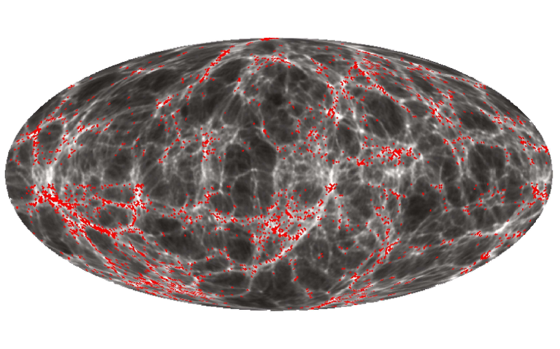
where the ensemble brackets denote angular averaging and $P_{\rm DM}(k)$ and $P_{\rm G}(k)$ are the associated power spectra. A cell-to-cell comparison of the logarithmic density fields in configuration space shows a typical Pearson coefficient of 74% for a cell width of $1.4\,\mbox{$h^{-1}$\,Mpc}$. The high degree of correlation between the 2MRS galaxy distribution and the reconstructed density field can be seen in Fig. 1. This plot shows a Mollview sky projection of all matter (grey scale) and galaxies (red dots) in our best-correlated real-space reconstruction at a distance of $50-60\,\mbox{$h^{-1}$\,Mpc}$. A remarkable spatial coincidence between the galaxy tracers and the underlying density field can be observed.

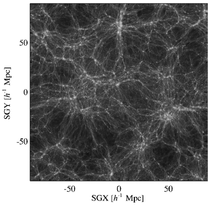
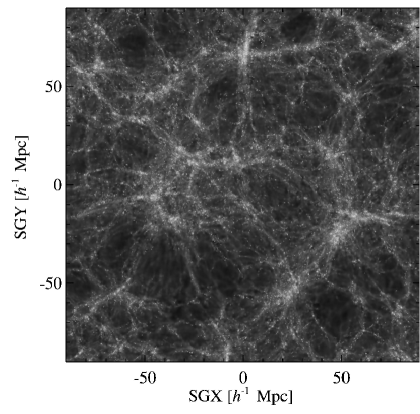
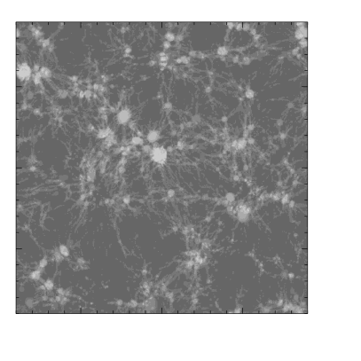
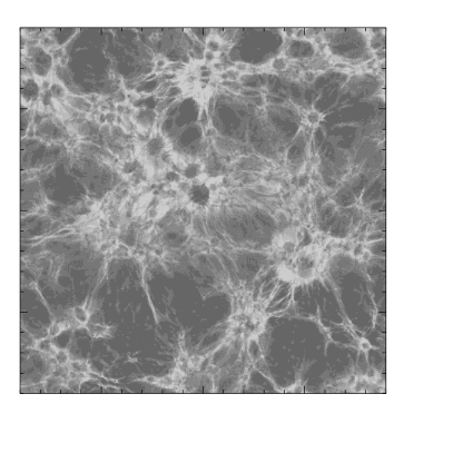
The difference between real and redshift space for our LU reconstruction can be seen in Fig. 2 (left and right panels respectively). This figure demonstrates the squashing effect produced along the line-of-sight as a result of the coherent peculiar motions of galaxies. In this sense, it is important to perform the cosmic web analysis both in configuration and redshift space in order to check for differences in the results. These runs are complemented with an analogous set of DM-only simulations carried out using unconstrained random phases for the ICs adopting the same cosmology and simulation parameters. This set of unconstrained simulations will serve to assess the level of cosmic variance of the LU reconstructions. The reader is referred to Heß et al. (2013) for further details.

A flat $\Lambda$CDM model consistent with WMAP7 results (Komatsu et al., 2011) was considered in these simulations, i.e. with a matter density $\Omega_{\rm M}=0.272$, a cosmological constant density of $\Omega_{\Lambda}=0.728$, a baryon density of $\Omega_{\rm b}=0.046$, a dimensionless Hubble constant $h=0.704$, an amplitude of mass fluctuations $\sigma_{8}=0.807$ and a scalar spectral index $n_{\rm s}=0.967$. The simulations were initialised at redshift $z=100$ and were evolved with the gadget-3 code (Springel, 2005; Springel et al., 2008) using $384^{3}$ particles, which translates into a DM particle mass of $7.8\times 10^{9}\,\mbox{$h^{-1}\,{\rm M}_{\odot}$}$, and a comoving gravitational softening of $15\,\mbox{$h^{-1}$\,kpc}$. Throughout this paper, we will use the density fields of the $N$-body simulations obtained from their corresponding DM distribution using a standard cloud-in-cell technique. The volume has been gridded with $128^{3}$ cells thus giving a cell side length of about $1.4\,\mbox{$h^{-1}$\,Mpc}$.

DM haloes in the simulations are identified using the ahf code (Knollmann & Knebe, 2009) as spherical overdensities with a density $200$ times above the critical density of the universe. In this way, a halo sample with masses in the range $\sim$$10^{11}-10^{14}\,\mbox{$h^{-1}\,{\rm M}_{\odot}$}$ was selected for our LU reconstructions (see Fig. 10 of Heß et al., 2013, for the mass function of our constrained realisations). To test for resolution and cosmology effects, when haloes are considered, we also used a higher resolution reconstruction with $768^{3}$ particles within the Planck cosmology (with $\Omega_{\rm M}=0.307$; Planck Collaboration et al., 2013), which results in a DM particle mass of $1.1\times 10^{9}\,\mbox{$h^{-1}\,{\rm M}_{\odot}$}$.

Figure 3: Matter density parameter as a function of radius for increasingly larger spheres as obtained from our reconstruction of the LU. Shown are the results corresponding to the DM as well as the halo contribution for virial halo mass cuts of $M_{\rm vir}>10^{12}$ and $5\times 10^{12}\,\mbox{$h^{-1}\,{\rm M}_{\odot}$}$ (black and blue lines respectively). Also shown are the observational results of Karachentsev (2012) which have been estimated from an updated local galaxy sample (circles). The solid circle with error bars stands for the integrated observational result within $50\,\mbox{Mpc}$ ($\equiv 35\,\mbox{$h^{-1}$\,Mpc}$).

3 Matter content in the LU: haloes vs. field

Throughout the years there have been claims that the LU may not be a fair sample of the Universe after studying the contribution of galaxy groups to its DM content. Typically these estimates place the local matter density value in the range $\Omega_{\rm M,LU}\approx 0.05-0.2$, i.e. below the cosmological mean density by a factor of a few (see e.g. Karachentsev 2012 and references therein). These results have been sometimes interpreted as the consequence of an underlying ‘missing DM problem’ that could potentially be in conflict with the $\Lambda$CDM cosmological model. In particular, the recent study of Karachentsev (2012) presents an updated analysis of a sample of local galaxies – that includes dwarfs, pairs, triplets and larger groups – favouring an estimate of $\Omega_{\rm M,LU}=0.08\pm 0.02$ for the volume contained within a distance of $50\,$Mpc.

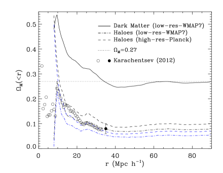
The amount of DM as a function of volume in our reconstructions can be straightforwardly checked for consistency with observational results. This is shown in Fig. 3 where the cumulative matter density parameter is calculated as a function of distance to the observer for our best (real-space) $N$-body reconstruction. It can be seen that the DM density shows some modulation owing to the particular LU realisation to finally converge to the mean cosmological value at a distance of about $60\,\mbox{$h^{-1}$\,Mpc}$, i.e. approximately $85\,$Mpc. The Local Void manifests itself as a slight trough in the cumulative matter density for distances of about $30-60\,\mbox{$h^{-1}$\,Mpc}$. This clearly indicates that the observed DM density estimates in the LU cannot be the result of cosmic variance as the corresponding minimum value in our reconstruction is well above $\Omega_{\rm M}=0.1$.

The situation changes if we consider the contribution of dark haloes alone. The dot-dashed (dashed) lines show the density parameter obtained from matter located within the virial radius of haloes for virial mass cuts of $M_{\rm vir}>10^{12}$ and $5\times 10^{12}\,\mbox{$h^{-1}\,{\rm M}_{\odot}$}$ (black and blue lines respectively) for the low (high) resolution $N$-body reconstruction. These cuts are roughly consistent with the minimum virial mass value of galaxy groups with $N>3$ in the Karachentsev (2012) sample as can be inferred from their Fig. 2. According to this work, these systems are the main contributors to the cosmic matter budget in the LU and have a median virial mass of about $1.69\times 10^{12}\,\mbox{$h^{-1}\,{\rm M}_{\odot}$}$ (Makarov & Karachentsev, 2011). In general, for the reconstructed halo samples, the predictions of both constrained simulations using different matter density parameters ($\Omega_{\rm M}=0.272$ and $\Omega_{\rm M}=0.307$, respectively) are compatible with the observational estimates of Karachentsev (2012) within the error bars.

Figure 4: VFF (left panel) and MFF (right panel) of our best correlated LU reconstruction in real space as a function of threshold eigenvalue for the T- and ${\rm div}\,$V-web cosmic web classification methods. Different environments are indicated.

Interestingly, the halo-derived matter density shape is similar to that obtained when all matter is taken into account. In particular, we are able to reproduce the observed increase in matter density as the scale radius decreases, an effect that is particularly prominent in our Local Volume (LV, i.e. $r\lesssim 20\,\mbox{$h^{-1}$\,Mpc}$). Additionally, the simulated halo matter density shows similar bumps to observations at distances of about $10-30\,\mbox{$h^{-1}\,{\rm M}_{\odot}$}$ which are mainly owing to the presence of the Local Supercluster. At scales below $10\,\mbox{$h^{-1}$\,Mpc}$, the mismatch between data and the matter density of haloes is likely owing to a combination of the limited resolution of our simulation and the uncertainties present in the selection function used in the reconstruction.

These results demonstrate that the ‘missing DM’ in the LU can be simply interpreted as being located outside massive haloes, i.e. forming part of the cosmic web ‘field’ in agreement with the $\Lambda$CDM expectations. This interpretation is strengthened by the results of Section 4.3. There it will be shown that, irrespective of the cosmic web classification used, most of the mass is located outside the densest regions.

Figure 5: Cosmic web density field of our best-correlated LU reconstruction in real space as obtained with the T-web method using $\lambda_{\rm th}=0.9$ for filaments (upper left), knots (upper right), sheets (lower left) and voids (lower right) in a slice of $7\,\mbox{$h^{-1}$\,Mpc}$. The different web structures are shown in light colours. The resulting VFFs of the web elements are about 7.6%, 0.6%, 20.4% and 71.4% respectively (see Section 4.3). Units are in supergalactic coordinates.

4 The cosmic web of the Local Universe

To carry out the cosmic web characterisation of the LU we apply to our reconstruction the tidal field tensor classification proposed by Hahn et al. (2007). In addition, we also explore the possibility of using the reconstructed nonlinear velocity field to perform the classification. Throughout this paper, we will refer to these approaches as the ‘T-web’ and ‘${\rm div}\,$V-web’ respectively. These methods are implemented within the classic software package, which will be presented in a forthcoming publication (Kitaura & Nuza, in preparation).

4.1 The ‘T-web’ method:

We study the dynamics of matter by computing the eigenvalues $\lambda_{i}$ $(i=1,2,3)$ of the tidal field tensor

$$T_{ij}\equiv\frac{\partial^{2}\phi_{\rm rec}}{\partial x_{i}\partial x_{j}},$$ (2)

where $\phi_{\rm rec}$ is the gravitational potential of the reconstructed nonlinear density field. By analysing the signature of the eigenvector $\vec{\lambda}=(\lambda_{1},\lambda_{2},\lambda_{3})$ at a given spatial point it is then possible to distinguish between different dynamical behaviours. For instance, collapsing (expanding) structures in all spatial dimensions will be classified as halo-like (void-like) regions. In a similar way, elongated-like (sheet-like) structures can be identified in the case of a 1-dimensional (2-dimensional) expansion. In what follows, we will designate to these four cases as knots, voids, filaments and sheets respectively.

However, not all positive (negative) eigenvalues will give rise to an actual collapse (expansion) along the corresponding axis in the inmediate future. Therefore, to achieve a more realistic correspondence between the tidal field tensor dynamical classification and the actual cosmic web we followed the approach of Forero-Romero et al. (2009): we classify structures according to the number of eigenvalues ($N_{\lambda}$) above a certain threshold ($\lambda_{\rm th}$) which, in general, will be nonzero. As a consequence, cells with $N_{\lambda}=3,2,1,0$ will then be classified as knots, filaments, sheets and voids, respectively.

4.2 The ‘div V-web’ method:

As an alternative way of performing the cosmic web classification, we use the information of the reconstructed nonlinear velocities alone. By taking the divergence of the velocity field we can infer the expected density distribution under the linear approximation. Specifically, the linear density field is obtained by computing

$$\delta_{\rm lin}=-\frac{\nabla\cdot{\bf{v}_{\rm rec}}}{fHa},$$ (3)

where $\bf{v}_{\rm rec}$ is the reconstructed nonlinear velocity field, $f$ is the logarithmic derivative of the linear growth factor, $H$ is the Hubble constant and $a$ is the expansion factor. Then, for computing the web, we use the corresponding linear potential as an input of the tidal field tensor classification method discussed above.

It is worth noting that in this method – as well as in any other classification derived from the velocity field – caution must be taken when considering knots, as shell crossing is known to dramatically affect the gridded peculiar velocity field (see e.g., Hoffman et al. 2012; Hahn et al. 2014).

4.3 Cosmic web statistics

Fig. 4 shows the volume and mass filling fractions (VFFs and MFFs respectively) of the simulated LU as a function of threshold eigenvalue for the best-correlated LU reconstruction of Heß et al. (2013) in real space as obtained from the T-web (upper panels) and ${\rm div}\,$V-web (lower panels) classification methods. As expected, the relative fraction of occupied volume and mass of the different structures vary as the threshold eigenvalue is increased. Interestingly, the VFFs for the two classification methods studied show somewhat similar values for a given eigenvalue threshold. Nevertheless, differences can be large for $\lambda_{\rm th}\approx 0$. For larger thresholds typical differences are of the order of $10-20\%$. This is not the case, however, for the MFFs. Despite showing the same trends, the amount of mass in each environment can be significantly different between the two methods. This is because the ${\rm div}\,$V-web classification linearises the density field thus removing material from the densest regions. As a result, the amount of mass in the classified knots and filaments is dramatically reduced, whereas the opposite occurs in sheets and voids. This is not surprising as the two classification methods considered probe different density regimes. Therefore, we do not expect a match between the corresponding statistics. In what follows, however, we plan to apply both cosmic web ‘finders’ to our reconstructed LU to assess the robustness of our conclusions.

4.3.1 Effective threshold

To choose the effective threshold eigenvalue defining the cosmic web, we rely on results of alternative classification methods. In particular, our aim is to reproduce the VFF of voids in a $\Lambda$CDM universe which is found to be considerably larger than about $17\%$, i.e. the value obtained in the pioneering classification of Hahn et al. (2007). In general, such alternative methods predict a void VFF in the range $70-90\%$. Techniques based on phase-space tesselations of the particle distribution have been used to classify voids as regions free of shell crossings (Abel et al., 2012; Falck et al., 2012; Shandarin et al., 2012). In this way, Shandarin et al. (2012) have shown that the volume fraction occupied by voids could be as high as $93\%$. However, as noted by Abel et al. (2012), these estimates must be taken with caution as they are strongly dependent on resolution. Other works, based on dynamical and/or kinematical approaches, present somewhat smaller values. For instance, by analysing the velocity shear tensor, Hoffman et al. (2012) presents a cosmic web classification resulting in a $69\%$ of voids. More recently, Cautun et al. (2013) performed a multiscale method, which includes a density filtering in logarithmic space, predicting a void VFF of $78\%$. This diversity in the VFFs hints at the complexity in the classification of the cosmic web. Therefore, in this work, we adopt a simple approach: we choose a threshold eigenvalue of $\lambda_{\rm th}=0.9$ to reproduce a void VFF within the range of estimates mentioned above in our unconstrained simulations. The same parameter is then consistently used in our reconstructions. As a result of this choice the remaining cosmic web structures (i.e., knots, filaments and sheets) will be uniquely determined as can be inferred from Fig. 4. We have checked that adopting other values – that will modify the corresponding void VFF – does not change the validity of our conclusions.

Figure 6: Cumulative VFF of the best-correlated reconstructed LU as a function of distance from the centre of the box for different environments. The cosmic web has been computed using the T-web method for a threshold of $\lambda_{\rm th}=0.9$. The inset plots show the results obtained using the div V-web classification with $\lambda_{\rm th}=0.8$. The error bars show the standard deviation of our ensemble of 25 reconstructions. The shaded regions represent the 1$\sigma$ cosmic variance fluctuations as obtained from unconstrained $N$-body simulations by placing 1000 ‘observers’ at different locations within the box, whereas the dotted line stands for the mean value.

Figure 7: Idem as Fig. 6 for the cumulative MFF.

4.3.2 Reconstructed filling fractions

After applying the T-web classification with $\lambda_{\rm th}=0.9$ to our best-correlated $N$-body reconstruction in configuration space, we obtain VFFs of about $71.4\%$, $20.4\%$, $7.6\%$, $0.6\%$ for voids, sheets, filaments and knots respectively. Similarly, the corresponding MFFs for these structures are of about $21.9\%$, $21.7\%$, $34.1\%$, $22.3\%$. We also found that, given the resolution adopted here, the resulting statistics are not significantly affected if the cosmic web classification is performed in redshift space. Fig. 5 shows a projection of the different cosmic web environments in the LU as determined by the T-web classification using $\lambda_{\rm th}=0.9$ for our best-correlated reconstruction in real space. These plots show a slice containing the supergalactic plane within a box of $180\,\mbox{$h^{-1}$\,Mpc}$ on a side that is centred in the observer’s position.

To compare the two classification methods considered here we use, for the ${\rm div}\,$V-web method, an eigenvalue threshold of $\lambda_{\rm th}=0.8$, aiming at approximately obtaining the same VFF of voids as with the T-web. In this case, the resulting VFFs and MFFs are of about $66.7\%$, $27.3\%$, $5.6\%$, $0.38\%$ and $29.3\%$, $43.5\%$, $24.9\%$, $2.4\%$ for voids, sheets, filaments and knots respectively for the same LU reconstruction. The small MFFs obtained for knots in this case clearly indicates that the ${\rm div}\,$V-web classification fails in characterising the densest regions, as expected.

5 Cosmic variance in the LU

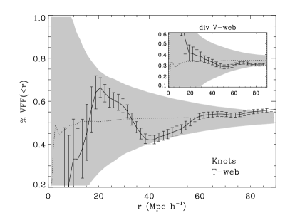
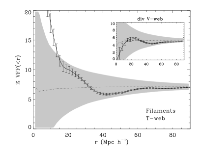
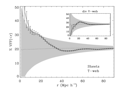
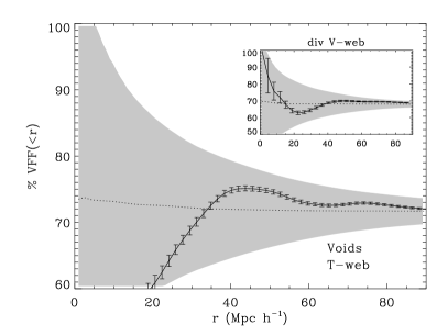
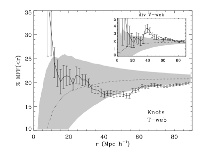
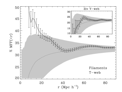
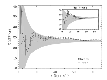
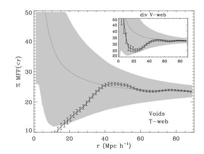
We compare the volume and mass statistics of the reconstructed cosmic web with those of the random simulations to assess the cosmic variance in the LU. Therefore, the particular method used to characterise the cosmic web is not relevant, as soon as the same method is applied to both sets of simulations. This can be seen in Figs. 6 and 7 for the T- and ${\rm div}\,$V-web classifications. The latter method is shown as inset plots to readily compare between the two web ‘finders’ in each case. The different panels show the cumulative VFFs (MFFs) of knots (upper-left panel), filaments (upper-right panel), sheets (lower-left panel) and voids (lower-right panel) as a function of distance to the observer, where the solid lines indicate the results for our best-correlated reconstruction in real space and the error bars (standard deviation) have been estimated using our ensemble of 25 reconstructions. To construct these plots we spherically averaged the corresponding filling fractions for a given scale to simplify the description of the problem. The grey shaded regions indicate the 1$\sigma$ cosmic variance level of an ordinary $\Lambda$CDM universe, built by placing 1000 ‘observers’ at different locations within our random set of unconstrained $N$-body simulations, whereas dotted lines indicate the mean value. We have checked that our results are marginally affected if, instead, we compute these statistics in redshift space, given the adopted resolution in our study. (Nevertheless, the impact of redshift-space distortions will be further considered in Section 6.) The first conclusion we can extract from these plots is that the LU is completely consistent with the expectations of $\Lambda$CDM, i.e. the measured LU statistics are well within the predicted 1$\sigma$ fluctuations of the concordance model at most of the studied scales and environments (despite of some departures for distances smaller than $\sim$15 $h^{-1}$ Mpc where the selection function is less constrained). Irrespective of the classification, some remarkable features are evident for $r\gtrsim 20\,\mbox{$h^{-1}$\,Mpc}$, i.e. as one increases the distance from the observer. At smaller scales, however, we found some differences between our two cosmic web methods. Since at these scales the selection function is not well constrained, in what follows, we will mainly focus on the results at $r\gtrsim 20\,\mbox{$h^{-1}$\,Mpc}$. In particular, for a sphere of radius $r=20\,\mbox{$h^{-1}$\,Mpc}$ the VFF of our reconstructed web is dominated by voids, occupying around $60\%$ of the volume, followed by sheets and filaments, that comprise $30-35\%$ and $5-10\%$ of the available space respectively. These values represent a fluctuation of about $1\sigma$ with respect to the expected mean of a $\Lambda$CDM universe, which is about $70-72\%$ for voids, $20-25\%$ for sheets and $5-7\%$ for filaments at this scale. High density regions, as characterised by knots, occupy less than $1\%$ of the volume, which is close to the expectation for an unconstrained universe. Despite the fact that the LV is mainly populated by sheets/voids, our immediate vicinity shows a smaller fraction of void-like regions in comparison to the mean $\Lambda$CDM expectation. This behaviour is, however, inverted for matter inside spheres with radius between $30-60\,\mbox{$h^{-1}$\,Mpc}$, where the VFF is above (below) the mean expectation in the case of voids (sheets, filaments and knots) reaching a peak (dip) at a distance of about $40\,\mbox{$h^{-1}$\,Mpc}$. This indicates that, at that particular radius, the fraction of voids is higher than average, thus contributing with more voids to the corresponding VFF. As expected, for increasingly larger spheres, the VFFs of the different cosmic web structures converge to the global mean value of the whole reconstruction. This behaviour is also observed for the MFF case, where we find results consistent with $\Lambda$CDM for radii greater than $\sim$$15\,\mbox{$h^{-1}$\,Mpc}$. In this case, however, the trends in the cumulative mass fractions present some differences between the two web ‘finders’. In fact, these discrepancies are expected as the cosmic web resulting from different approaches do not completely overlap (e.g., Cautun et al., 2013). This is most noticeable for knots owing to the field linearisation carried out in the ${\rm div}\,$V-web classification. However, this effect generates differences in other cosmic web structures as well. Therefore, this fact prevents us from making strong conclusions about the cumulative MFF profile in these environments. Nevertheless, we can safely conclude that, irrespective of the classification, the LU is in agreement with the expected $\Lambda$CDM fluctuations as our measured statistics are always contained within $1\sigma$ at scales $r\gtrsim 15\,\mbox{$h^{-1}$\,Mpc}$. In addition, we can state that, when considering a volume with a radius of about $60\,\mbox{$h^{-1}$\,Mpc}$, the LU becomes a fair sample thus converging to the mean $\Lambda$CDM expectations.

6 Environmental dependence of galaxy morphology

As a first application of our detailed LU reconstructions we use the 2MRS catalogue to correlate the position of galaxies with the environmental information provided by the cosmic web classifications computed in Section 4.3. To avoid any gridding effect all fields analysed here will be convolved with a Gaussian filter using a length of one cell. Nevertheless, we have checked that the resulting trends and significances are slightly affected if no smoothing is used.

We divide the observed galaxy sample in 4 broad categories according to the morphological type assigned by the 2MRS team, namely: ellipticals (E), lenticulars (S0), spirals (Sp) and irregulars (Irr). After selecting objects within the volume of the reconstruction we end up with a sample of 21,893 galaxies, out of which 8,367 correspond to ellipticals, 1,323 to lenticulars, 11,903 to spirals and 300 to irregulars. To every galaxy, we assign an environment corresponding to the cell where it is placed as determined by a given cosmic web classification method. Following Lee & Lee (2008), we define what we call the ‘excess probability ratio’ as

$$\eta(\mathcal{T}|\mathcal{E})\equiv\frac{\mathcal{P}(\mathcal{T}|\mathcal{E})}{\mathcal{P}(\mathcal{G}|\mathcal{E})},$$ (4)

where $\mathcal{G}$ represents a random galaxy in the volume, $\mathcal{T}$ is the galaxy type, $\mathcal{E}$ is the considered environment (knot, filament, sheet or void) and $\mathcal{P}(\mathcal{X}|\mathcal{Y})$ is the conditional probability of $\mathcal{X}$ given $\mathcal{Y}$. The interpretation of the excess probability ratio is therefore rather simple: if galaxies of a given type displayed some preference to be located in a particular environment then the excess probability ratio has to be $\eta(\mathcal{T}|\mathcal{E})>1$, whereas $\eta(\mathcal{T}|\mathcal{E})<1$ has to be true in the opposite situation. The case $\eta(\mathcal{T}|\mathcal{E})=1$ indicates no distinction from the random distribution.

To estimate the actual conditional probabilities we measure galaxy number counts provided by the 2MRS catalogue. Specifically, we approximate their values as $\mathcal{P}(\mathcal{T}|\mathcal{E})\approx N_{\rm g}(\mathcal{T}|\mathcal{E})/N_{\rm g}(\mathcal{T})$ and $\mathcal{P}(\mathcal{G}|\mathcal{E})\approx N_{\rm g}(\mathcal{E})/N_{\rm tot}$, where $N_{\rm g}(\mathcal{Z})$ is the number of galaxies satisfying the condition $\mathcal{Z}$ and $N_{\rm tot}$ is the total number of galaxies in our sample. Therefore, our estimator for the excess probability presented in Eq. (4) results in

$$\eta(\mathcal{T}|\mathcal{E})\approx\frac{N_{\rm g}(\mathcal{T}|\mathcal{E})N_{\rm tot}}{N_{\rm g}(\mathcal{T})N_{\rm g}(\mathcal{E})}.$$ (5)

Figure 8: ‘Excess probability’ $\eta(\tau,\epsilon)$ in redshift space for a galaxy of a given morphological type $\tau$ (i.e., E: elliptical; S0: lenticular; Sp: spiral; Irr: irregular) to inhabit a particular environment as indicated in the panels. Results are presented for the T-web (solid circles) and div V-web (open circles) classification methods using a threshold of $\lambda_{\rm th}=0.9$ and $0.8$ respectively. The error bars are computed assuming Poisson statistics. Also shown is the excess probability with respect to the null signal (as represented by the dashed lines) measured, in each case, in units of the standard deviation, where the light (dark) shaded regions represent the 1$\sigma$ (2$\sigma$) levels.

Figure 9: Idem as Fig. 8 but in real space. A mapping between the real- and redshift-space reconstruction has been used to assign the most likely real-space position to every 2MRS galaxy (see text).

The shot noise contribution of the number counts is modelled assuming Poisson statistics thus allowing us to estimate the magnitude of the associated errors.

6.1 Correlations in redshift space

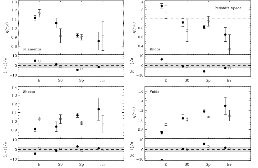
Fig. 8 shows the resulting excess probabilities of the different galaxy morphologies within the cosmic web for the redshift-space LU reconstruction. In this way, we can directly compare the reconstruction to observations. To compute the excess probability signal we use both the T-web and div V-web classification methods. In the first place, it can be seen that there is a global tendency for elliptical galaxies to preferentially reside in knots and in filaments rather than in sheets and voids. This trend is inverted in the case of spiral and irregular galaxies. This can be more clearly seen in the T-web case whereas, when adopting the div V-web method to define the web, the error bars tend to increase thus erasing the signal corresponding to spirals. However, quite generally, lenticular galaxies display no preference for a particular environment irrespective of the classification method. These measurements provide the strength of the tendency to inhabit/avoid a certain environment. According to the T-web classification, which provides the most significant detections, it can be seen that ellipticals are most easily found in knots ($\eta=1.29\pm 0.05$) than in filaments ($\eta=1.11\pm 0.03$) whereas they tend to avoid sheets ($\eta=0.91\pm 0.02$) less than voids ($\eta=0.73\pm 0.03$). On the contrary, spirals are most commonly found in voids ($\eta=1.18\pm 0.03$) than in sheets ($\eta=1.07\pm 0.02$) whereas they tend to avoid filaments ($\eta=0.92\pm 0.02$) less than knots ($\eta=0.82\pm 0.03$). In general, irregular galaxies follow the same trends as spirals although, in this case, the error bars are larger as a result of their smaller number in our sample. For ellipticals, the significance of the corresponding signals – according to the T-web (div V-web) classification – result in: $5.5\sigma\,(1.1\sigma)$, $4.3\sigma\,(3.9\sigma)$, $3.8\sigma\,(1.1\sigma)$ and $9.7\sigma\,(4.1\sigma)$ for knots, filaments, sheets and voids, respectively. Similarly, for spirals, we obtain significances of $5.4\sigma\,(0.5\sigma)$, $4.1\sigma\,(3.3\sigma)$, $2.8\sigma\,(1\sigma)$ and $5.2\sigma\,(2.7\sigma)$ for the corresponding environments.

6.2 Correlations in configuration space

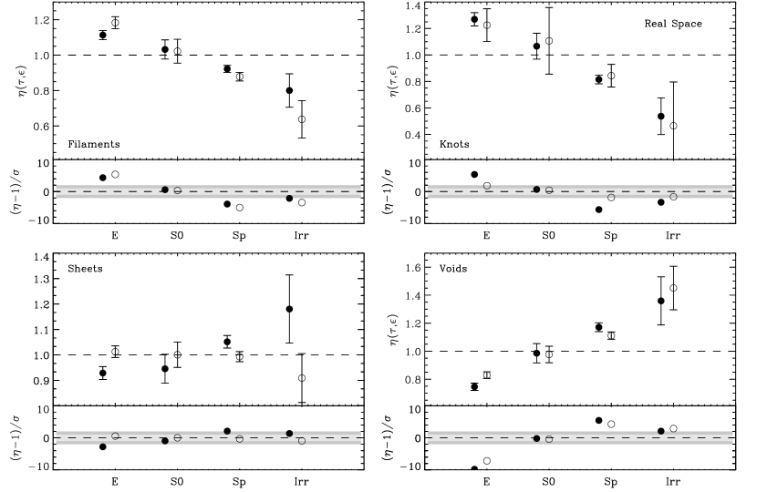
As an additional exercise we also computed the probability ratios using the reconstructed real-space reconstruction as shown in Fig. 9. To compare our reconstruction with observations, we transformed the observed data from redshift to real space. This is, in general, not a trivial task although, using our reconstructions, it is possible to establish a mapping between redshift and configuration space (see Fig. 2). Specifically, we use our set of constrained haloes in real and redshift space to estimate the most likely real-space position of the corresponding observed 2MRS galaxies. In particular, for each galaxy, we search for the closest halo in redshift space using our ensemble of cosmological simulations, and assign the associated real-space position of the halo. As can be seen from Fig. 9, the excess probability correlations in real space display, in general, the same trends discussed before. However, some new features are worth mentioning. In this case, the correlations show a smaller scatter, typically decreasing the size of the error bars. Moreover, the $\eta$-morphology relations derived using the T-web and the ${\rm div}\,$V-web get more consistent with each other. This is mainly owing to the fact that working in configuration space reduces the artificial shell crossing caused by redshift-space distortions. For ellipticals, in real space, the significance of the corresponding signals – according to the T-web (div V-web) classification – are: $5.3\sigma\,(1.8\sigma)$, $4.3\sigma\,(5.3\sigma)$, $2.8\sigma\,(0.5\sigma)$ and $9.8\sigma\,(7.2\sigma)$ for knots, filaments, sheets and voids, respectively. Similarly, for spirals, we obtain significances of $5.6\sigma\,(1.8\sigma)$, $3.9\sigma\,(5\sigma)$, $2.1\sigma\,(0.3\sigma)$ and $5.4\sigma\,(4.3\sigma)$ for the corresponding environments. Note that, in general, the results for the T-web and div V-web methods are now more similar to each other than in the redshift-space case, as expected.

Interestingly, for a given environment, the excess probability displays a clear correlation as a function of galaxy type from ellipticals to irregulars, which provide insights to the process of galaxy formation and the build up of the Hubble sequence. The resulting slope in the $\eta$-morphology relation turns out to be positive in the sheet and void cases while it gets negative for filaments and knots. These trends are consistent with the idea of a continuous transition from irregular/spiral to elliptical morphology. The direction of the transition is suggested by the gradual increase of the slope as one follows the sequence knots–filaments–sheets–voids, i.e. from the more to the less dense environments. This indicates that spheroidal-like systems are most probably formed in high-density regions as a result of mergers between irregular/spiral objects. Conversely, the lower merger probability in less dense environments permits the latter to retain their morphology.

7 Summary and Conclusions

In this work we have presented a characterisation of the matter content of the LU including a cosmic web analysis and an environmental-galaxy morphology study based on a constrained cosmological simulation. This is only possible owing to the high-precision of the reconstructed initial conditions performed by the Bayesian self-consistent method of Kitaura (2013). Our reconstruction covers a volume of $180^{3}\,h^{-3}\,{\rm Mpc^{3}}$ and it was produced using the spatial information provided by 31,107 2MRS galaxies (Heß et al., 2013). To characterise the cosmic web of the reconstruction we have applied the tidal field tensor classification method on the nonlinear (T-web) and linear (div V-web) density fields separately (see Section 4). The latter has been computed using the reconstructed nonlinear velocity field within the linear theory approximation.

To estimate the expected cosmic variance level we used a suite of unconstrained $N$-body simulations with the same parameter setting as in our reconstructions. In this way, we were able to assess the consistency level of the specific LU realisation with the $\Lambda$CDM cosmology. To that end we have measured the corresponding VFFs and MFFs of voids, sheets, filaments and knots of the LU and compared them with those resulting from $N$-body universes with random initial seeds. This work brings up a number of novel aspects that are important to remark:

• We use a state-of-the-art reconstruction of the nonlinear density and peculiar velocity fields based on high precision constrained simulations that reach an accuracy of about 3 Mpc.
  

• Based on such a reconstruction we present the first fully nonlinear cosmic web classification of the LU using the tidal field tensor method on the reconstructed density field.
  

• For the first time, we use the reconstructed nonlinear peculiar velocity field to characterise basic statistics of the LU cosmic web as well as to perform a study on the relation between galaxy morphology and environment.
  

In what follows we summarise the main findings of our work:

• We measured the DM density profile in the LU by using our $N$-body reconstruction. As a result, we found that the so-called ‘missing DM problem’ can be simply interpreted as the consequence of ignoring matter located outside haloes above a given mass threshold. In fact, if we select simulated haloes with a similar virial mass cut as in the observations of Karachentsev (2012) (see also Makarov & Karachentsev 2011) we are able to reproduce the observed value within $50\,\mbox{Mpc}$ ($\Omega_{\rm M,LU}\approx 0.1$) and the shape of the profile (see Fig. 3). Instead, if we consider all matter present in the cosmic web, the matter density readily converges to the mean universal value. This suggests that the observationally-derived low matter density values cannot be the result of cosmic variance alone.
  

• Both the reconstructed VFF and MFF statistics, computed using increasingly larger spheres centred on the observer’s location, display, in general, a nice agreement with the expectations of $\Lambda$CDM. In particular, for a scale-radius larger than $r\gtrsim 15\,\mbox{$h^{-1}$\,Mpc}$ the deviations for all web environments are within $1\sigma$ of the expected cosmic variance. In particular, when considering a sphere with a radius of about $60\,\mbox{$h^{-1}$\,Mpc}$, these statistics converge to the mean value of the random $\Lambda$CDM realisations, thus representing a fair sample.
  

• We have measured the tendency of 2MRS galaxies to inhabit/avoid different environments as a function of morphology quantified in terms of the excess probability ratio $\eta$. In agreement with previous work, we found that elliptical systems are prone to be found in higher density regions, which we identify with knots and filaments in the web, rather than in sheets and voids. The opposite is true for spirals. In general, we found that the $\eta$-morphology correlations are best defined in real space where artificial shell crossing effects caused by redshift-space distortions are not present.
  

• In particular, if the T-web classification is adopted to define the cosmic web in our real-space reconstruction, elliptical galaxies show a clear signal ($\eta=1.27\pm 0.05$) to preferentially reside in clusters, at a $5.3\sigma$ level, as opposed to sheets ($\eta=0.93\pm 0.03$) and voids ($\eta=0.75\pm 0.03$), at a level of $2.8\sigma$ and $9.8\sigma$, respectively. Interestingly, we also found that elliptical galaxies show an excess probability of $\eta=1.11\pm 0.03$ in filaments that represents a $4.3\sigma$ detection. However, filaments in the tidal field classification are not very well defined in the vicinity of high density regions, as it is shown in Forero-Romero et al. (2009) (their Fig. 1). Therefore, the latter result should be taken with caution. For spiral galaxies, we found a tendency to reside in voids ($\eta=1.17\pm 0.03$) and sheets ($\eta=1.05\pm 0.02$) at a $5.4\sigma$ and $2.1\sigma$, as opposed to filaments ($\eta=0.92\pm 0.02$) and knots ($\eta=0.82\pm 0.03$), at a $3.9\sigma$ and $5.6\sigma$ level, respectively. If, instead, we use the div V-web classification to define the web we found that we can reproduce globally the same trends.
  

• Irrespectively of the classification adopted to define the web we found that, in general, lenticular (S0) galaxies in the 2MRS catalogue do not show a preference for any particular environment. Irregulars, on the contrary, show similar trends as in the spiral case, although at much lower significance as a result of the small galaxy number in our sample.
  

As a final remark, we would like to note that our results concerning the validity of $\Lambda$CDM have to be taken as a consistency check since the constrained simulations were performed assuming that very same model. It is nevertheless remarkable that our constrained simulations are able to provide an explanation to the properties of the LU by either cosmic variance or observational biases without invoking a paradigm shift in cosmology. In this regard, we want to emphasise that the phases of the primordial fluctuations in our reconstructions – which determine the location of peaks and troughs – are purely constrained by the data. This work demonstrates that high precision constrained simulations can indeed help to characterise the properties of the LU in different environments. Therefore, we anticipate a large number of applications in which galaxy formation can be tested by directly cross-correlating observations to simulations including the full phase-space information.

References

- Abel et al. (2012) Abel T., Hahn O., Kaehler R., 2012, MNRAS, 427, 61
- Alonso et al. (2006) Alonso M., Lambas D. G., Tissera P., Coldwell G., 2006, MNRAS, 367, 1029
- Alonso et al. (2012) Alonso S., Mesa V., Padilla N., Lambas D. G., 2012, A&A, 539, A46
- Aragon-Calvo (2012) Aragon-Calvo M. A., 2012, ArXiv e-prints
- Bahcall et al. (2000) Bahcall N. A., Cen R., Davé R., Ostriker J. P., Yu Q., 2000, ApJ, 541, 1
- Baldry et al. (2006) Baldry I. K., Balogh M. L., Bower R. G., Glazebrook K., Nichol R. C., Bamford S. P., Budavari T., 2006, MNRAS, 373, 469
- Ball et al. (2008) Ball N. M., Loveday J., Brunner R. J., 2008, MNRAS, 383, 907
- Balogh et al. (2004) Balogh M. L., Baldry I. K., Nichol R., Miller C., Bower R., Glazebrook K., 2004, ApJL, 615, L101
- Balogh et al. (2001) Balogh M. L., Christlein D., Zabludoff A. I., Zaritsky D., 2001, ApJ, 557, 117
- Beygu et al. (2013) Beygu B., Kreckel K., van de Weygaert R., van der Hulst J. M., van Gorkom J. H., 2013, AJ, 145, 120
- Blanton et al. (2005) Blanton M. R., Eisenstein D., Hogg D. W., Schlegel D. J., Brinkmann J., 2005, ApJ, 629, 143
- Bond et al. (1996) Bond J. R., Kofman L., Pogosyan D., 1996, Nature, 380, 603
- Branchini et al. (2012) Branchini E., Davis M., Nusser A., 2012, MNRAS, 424, 472
- Cautun et al. (2013) Cautun M., van de Weygaert R., Jones B. J. T., 2013, MNRAS, 429, 1286
- Ceccarelli et al. (2006) Ceccarelli L., Padilla N. D., Valotto C., Lambas D. G., 2006, MNRAS, 373, 1440
- Ceccarelli et al. (2013) Ceccarelli L., Paz D., Lares M., Padilla N., Lambas D. G., 2013, MNRAS, 434, 1435
- Cen & Ostriker (1993) Cen R., Ostriker J. P., 1993, ApJ, 417, 415
- Crook et al. (2007) Crook A. C., Huchra J. P., Martimbeau N., Masters K. L., Jarrett T., Macri L. M., 2007, ApJ, 655, 790
- Croton et al. (2005) Croton D. J., et al., 2005, MNRAS, 356, 1155
- Davis et al. (1985) Davis M., Efstathiou G., Frenk C. S., White S. D. M., 1985, ApJ, 292, 371
- de la Torre & Peacock (2013) de la Torre S., Peacock J. A., 2013, MNRAS, 435, 743
- de Vaucouleurs (1953) de Vaucouleurs G., 1953, AJ, 58, 30
- de Vaucouleurs et al. (1976) de Vaucouleurs G., de Vaucouleurs A., Corwin Jr. H. G., 1976, Second reference catalogue of bright galaxies. Containing information on 4,364 galaxies with references to papers published between 1964 and 1975.
- de Vaucouleurs et al. (1991) de Vaucouleurs G., de Vaucouleurs A., Corwin Jr. H. G., Buta R. J., Paturel G., Fouqué P., 1991, Third Reference Catalogue of Bright Galaxies. Volume I: Explanations and references. Volume II: Data for galaxies between 0h and 12h. Volume III: Data for galaxies between 12h and 24h.
- Deng et al. (2011) Deng X.-F., Chen Y.-Q., Jiang P., 2011, MNRAS, 417, 453
- Doroshkevich et al. (1980) Doroshkevich A. G., Kotok E. V., Poliudov A. N., Shandarin S. F., Sigov I. S., Novikov I. D., 1980, MNRAS, 192, 321
- Dressler (1980) Dressler A., 1980, ApJ, 236, 351
- Einasto et al. (2007) Einasto M., Einasto J., Tago E., Saar E., Liivamägi L. J., Jõeveer M., Hütsi G., Heinämäki P., Müller V., Tucker D., 2007, A&A, 464, 815
- Erdoǧdu et al. (2004) Erdoǧdu P., et al., 2004, MNRAS, 352, 939
- Erdoǧdu et al. (2006) Erdoǧdu P., et al., 2006, MNRAS, 368, 1515
- Falck et al. (2012) Falck B. L., Neyrinck M. C., Szalay A. S., 2012, ApJ, 754, 126
- Farouki & Shapiro (1981) Farouki R., Shapiro S. L., 1981, ApJ, 243, 32
- Forero-Romero et al. (2009) Forero-Romero J. E., Hoffman Y., Gottlöber S., Klypin A., Yepes G., 2009, MNRAS, 396, 1815
- Fry & Peebles (1978) Fry J. N., Peebles P. J. E., 1978, ApJ, 221, 19
- Górski et al. (2005) Górski K. M., Hivon E., Banday A. J., Wandelt B. D., Hansen F. K., Reinecke M., Bartelmann M., 2005, ApJ, 622, 759
- Hahn et al. (2014) Hahn O., Angulo R. E., Abel T., 2014, ArXiv e-prints
- Hahn et al. (2007) Hahn O., Porciani C., Carollo C. M., Dekel A., 2007, MNRAS, 375, 489
- Heß et al. (2013) Heß S., Kitaura F.-S., Gottlöber S., 2013, MNRAS
- Hoffman et al. (2012) Hoffman Y., Metuki O., Yepes G., Gottlöber S., Forero-Romero J. E., Libeskind N. I., Knebe A., 2012, MNRAS, 425, 2049
- Hogg et al. (2004) Hogg D. W., Blanton M. R., Brinchmann J., Eisenstein D. J., Schlegel D. J., Gunn J. E., McKay T. A., Rix H.-W., Bahcall N. A., Brinkmann J., Meiksin A., 2004, ApJL, 601, L29
- Hoyle & Vogeley (2004) Hoyle F., Vogeley M. S., 2004, ApJ, 607, 751
- Huchra et al. (2012) Huchra J. P., et al., 2012, ApJS, 199, 26
- Jasche et al. (2010) Jasche J., Kitaura F.-S., Li C., Enßlin T. A., 2010, MNRAS, 409, 355
- Jasche & Wandelt (2013) Jasche J., Wandelt B. D., 2013, MNRAS, 432, 894
- Karachentsev (2012) Karachentsev I. D., 2012, Astrophysical Bulletin, 67, 123
- Kauffmann et al. (2004) Kauffmann G., White S. D. M., Heckman T. M., Ménard B., Brinchmann J., Charlot S., Tremonti C., Brinkmann J., 2004, MNRAS, 353, 713
- Kitaura (2013) Kitaura F.-S., 2013, MNRAS, 429, L84
- Kitaura & Angulo (2012) Kitaura F.-S., Angulo R. E., 2012, MNRAS, 425, 2443
- Kitaura et al. (2012) Kitaura F.-S., Erdoǧdu P., Nuza S. E., Khalatyan A., Angulo R. E., Hoffman Y., Gottlöber S., 2012, MNRAS, 427, L35
- Kitaura & Heß (2013) Kitaura F.-S., Heß S., 2013, MNRAS
- Kitaura et al. (2009) Kitaura F.-S., Jasche J., Li C., Enßlin T. A., Metcalf R. B., Wandelt B. D., Lemson G., White S. D. M., 2009, MNRAS, 400, 183
- Knollmann & Knebe (2009) Knollmann S. R., Knebe A., 2009, ApJS, 182, 608
- Komatsu et al. (2011) Komatsu E., et al., 2011, ApJS, 192, 18
- Kreckel et al. (2012) Kreckel K., Platen E., Aragón-Calvo M. A., van Gorkom J. H., van de Weygaert R., van der Hulst J. M., Beygu B., 2012, AJ, 144, 16
- Lackner & Gunn (2013) Lackner C. N., Gunn J. E., 2013, MNRAS, 428, 2141
- Lee & Lee (2008) Lee J., Lee B., 2008, ApJ, 688, 78
- Lietzen et al. (2012) Lietzen H., Tempel E., Heinämäki P., Nurmi P., Einasto M., Saar E., 2012, A&A, 545, A104
- Magtesyan (1988) Magtesyan A. P., 1988, Astrophysics, 28, 150
- Makarov & Karachentsev (2011) Makarov D., Karachentsev I., 2011, MNRAS, 412, 2498
- Martínez et al. (2006) Martínez H. J., O’Mill A. L., Lambas D. G., 2006, MNRAS, 372, 253
- Muñoz-Cuartas et al. (2011) Muñoz-Cuartas J. C., Müller V., Forero-Romero J. E., 2011, MNRAS, 417, 1303
- Müller et al. (2000) Müller V., Arbabi-Bidgoli S., Einasto J., Tucker D., 2000, MNRAS, 318, 280
- Neyrinck (2013) Neyrinck M. C., 2013, MNRAS, 428, 141
- Nuza et al. (2010) Nuza S. E., Dolag K., Saro A., 2010, MNRAS, 407, 1376
- Oemler (1974) Oemler Jr. A., 1974, ApJ, 194, 1
- Pan et al. (2012) Pan D. C., Vogeley M. S., Hoyle F., Choi Y.-Y., Park C., 2012, MNRAS, 421, 926
- Park et al. (2007) Park C., Choi Y.-Y., Vogeley M. S., Gott III J. R., Blanton M. R., SDSS Collaboration 2007, ApJ, 658, 898
- Peebles (1980) Peebles P. J. E., 1980, The large-scale structure of the universe
- Planck Collaboration et al. (2013) Planck Collaboration Ade P. A. R., Aghanim N., Armitage-Caplan C., Arnaud M., Ashdown M., Atrio-Barandela F., Aumont J., Baccigalupi C., Banday A. J., et al. 2013, ArXiv e-prints
- Shandarin et al. (2012) Shandarin S., Habib S., Heitmann K., 2012, Phys. Rev. D, 85, 083005
- Smith et al. (2012) Smith A. G., Hopkins A. M., Hunstead R. W., Pimbblet K. A., 2012, MNRAS, 422, 25
- Sousbie et al. (2008) Sousbie T., Pichon C., Courtois H., Colombi S., Novikov D., 2008, ApJL, 672, L1
- Sousbie et al. (2011) Sousbie T., Pichon C., Kawahara H., 2011, MNRAS, 414, 384
- Springel (2005) Springel V., 2005, MNRAS, 364, 1105
- Springel et al. (2008) Springel V., Wang J., Vogelsberger M., Ludlow A., Jenkins A., Helmi A., Navarro J. F., Frenk C. S., White S. D. M., 2008, MNRAS, 391, 1685
- Stoica et al. (2010) Stoica R. S., Martínez V. J., Saar E., 2010, A&A, 510, A38
- Sutter et al. (2012) Sutter P. M., Lavaux G., Wandelt B. D., Weinberg D. H., 2012, ApJ, 761, 44
- Sutter et al. (2013) Sutter P. M., Lavaux G., Wandelt B. D., Weinberg D. H., Warren M. S., 2013, ArXiv e-prints
- Tanaka et al. (2004) Tanaka M., Goto T., Okamura S., Shimasaku K., Brinkmann J., 2004, AJ, 128, 2677
- Tavasoli et al. (2013) Tavasoli S., Vasei K., Mohayaee R., 2013, A&A, 553, A15
- Tempel et al. (2011) Tempel E., Saar E., Liivamägi L. J., Tamm A., Einasto J., Einasto M., Müller V., 2011, A&A, 529, A53
- Tempel et al. (2014) Tempel E., Stoica R. S., Martínez V. J., Liivamägi L. J., Castellan G., Saar E., 2014, MNRAS, 438, 3465
- Toomre & Toomre (1972) Toomre A., Toomre J., 1972, ApJ, 178, 623
- Tully (1987) Tully R. B., 1987, ApJ, 321, 280
- Tully & Fisher (1987) Tully R. B., Fisher J. R., 1987, Nearby galaxies Atlas
- van der Wel (2008) van der Wel A., 2008, ApJL, 675, L13
- Vennik (1984) Vennik J., 1984, Tartu Astrofuusika Observatoorium Teated, 73, 1
- Wang et al. (2013) Wang H., Mo H. J., Yang X., van den Bosch F. C., 2013, ApJ, 772, 63
- Weinmann et al. (2006) Weinmann S. M., van den Bosch F. C., Yang X., Mo H. J., 2006, MNRAS, 366, 2
- Wetzel et al. (2012) Wetzel A. R., Tinker J. L., Conroy C., 2012, MNRAS, 424, 232
- White & Rees (1978) White S. D. M., Rees M. J., 1978, MNRAS, 183, 341
- Yahil et al. (1991) Yahil A., Strauss M. A., Davis M., Huchra J. P., 1991, ApJ, 372, 380
- Zandivarez & Martínez (2011) Zandivarez A., Martínez H. J., 2011, MNRAS, 415, 2553
- Zaroubi et al. (1999) Zaroubi S., Hoffman Y., Dekel A., 1999, ApJ, 520, 413
- Zel’dovich (1970) Zel’dovich Y. B., 1970, A&A, 5, 84