Investigation of the stellar content in the western part of the Carina nebula

Abstract

Context. The low obscuration and proximity of the Carina nebula make it an ideal place to study the ongoing star formation process and impact of massive stars on low-mass stars in their surroundings.

Aims. To investigate this process, we generated a new catalog of the pre-main-sequence (PMS) stars in the Carina west (CrW) region and studied their nature and spatial distribution. We also determined various parameters (reddening, reddening law, age, mass), which are used further to estimate the initial mass function (IMF) and $K$-band luminosity function (KLF) for the region under study.

Methods. We obtained deep $UBVRI$ $H\alpha$ photometric data of the field situated to the west of the main Carina nebula and centered on WR 22. Medium-resolution optical spectroscopy of a subsample of X-ray selected objects along with archival data sets from $Chandra$, $XMM-Newton$ and 2MASS surveys were used for the present study. Different sets of color-color and color-magnitude diagrams are used to determine reddening for the region and to identify young stellar objects (YSOs) and estimate their age and mass.

Results. Our spectroscopic results indicate that the majority of the X-ray sources are late spectral type stars. The region shows a large amount of differential reddening with minimum and maximum values of $E(B-V)$ as 0.25 and 1.1 mag, respectively. Our analysis reveals that the total-to-selective absorption ratio $R_{V}$ is $\sim$3.7 $\pm$ 0.1, suggesting an abnormal grain size in the observed region. We identified 467 YSOs and studied their characteristics. The ages and masses of the 241 optically identified YSOs range from $\sim$0.1 to 10 Myr and $\sim$0.3 to 4.8 M_⊙, respectively. However, the majority of them are younger than 1 Myr and have masses below 2 M_⊙. The high mass star WR 22 does not seem to have contributed to the formation of YSOs in the CrW region. The initial mass function slope, $\Gamma$, in this region is found to be $-$1.13 $\pm$ 0.20 in the mass range of 0.5 $<$ M/M_⊙ $<$ 4.8. The $K$-band luminosity function slope ($\alpha$) is also estimated as 0.31 $\pm$ 0.01. We also performed minimum spanning tree analysis of the YSOs in this region, which reveals that there are at least ten YSO cores associated with the molecular cloud, and that leads to an average core radius of 0.43 pc and a median branch length of 0.28 pc.

1 Introduction

Massive stars (M $>$ 8$-$10 M_⊙) in star-forming regions significantly influence their surroundings. In the course of their life, the feedback provided by their energetic ionization radiation and powerful stellar winds regulate the formation of low- and intermediate-mass stars (Garay & Lizano, 1999; Zinnecker & Yorke, 2007). After a short life time ($\lesssim$10⁷ years), they explode as supernovae or hypernovae (supernovae with substantially higher energy than standard supernovae) enriching the interstellar medium with the products of the various nucleosynthesis processes that have occurred during their lifetime (see Arnett, 1995, 1996; Woosley & Weaver, 1995; Nomoto et al., 2003, and references therein). The shock waves produced in these events may trigger new star formation (e.g. Elmegreen, 1998). Characterizing the young stellar objects (YSOs) in massive star-forming regions is therefore of utmost importance to understand the link with the neighboring massive star population.

The Carina nebula (NGC 3372) region, which hosts several young star clusters made of very massive stars along with YSOs, provides an ideal laboratory for studying the ongoing star formation (see Smith & Brooks, 2008). The CO survey of this region demonstrates that the Carina nebula is on the edge of a giant molecular cloud extending over $\sim$130 pc and has a mass in excess of 5 $\times$ 10⁵ M_⊙ (see Grabelsky et al., 1988). It contains $\sim$200 OB stars (Smith, 2006a; Povich et al., 2011), more than $\sim$60 massive O stars (see Feinstein, 1995; Smith, 2006a), and three WN(H) stars (i.e. WR 22, 24, and 25; Smith 2006a; Smith & Brooks 2008).

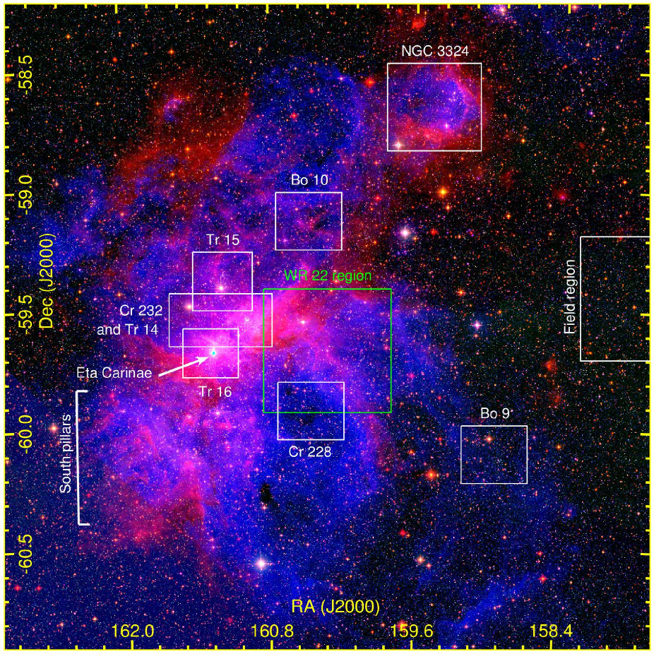
Figure 1: Color composite image of the large ($2.7^{\circ}\times 2.7^{\circ}$) area containing the Carina Nebula and centered at $\alpha$(J2000) = 10^h 41^m 17$\aas@@fstack{s}$5 and $\delta(J2000)=-59\degr\leavevmode\nobreak\ 40\arcmin\leavevmode\nobreak\ 36\aas@@fstack{\prime\prime}9$. This RGB image was made using the WISE 4.6 $\mu$m (red), 2MASS $K_{s}$ band (green), and DSS $R$ band (blue) images. Approximate locations of different star clusters (Tr 14, 15, 16; Bo 9, 10; Cr 228, 232, and NGC 3324) are denoted by white boxes. $\eta$ Carinae is marked by an arrow and in the lower left part of the image, south pillars (Smith et al., 2000) are shown. The region covered in the present study is shown by the green box. Part of the selected field region can be seen in the extreme western part of the image. North is up and east is to the left.

Initially, on the basis of infrared (IR) and molecular studies of the central Carina region, several authors (see Harvey et al., 1979; Ghosh et al., 1988; de Graauw et al., 1981; Cox, 1995) have reported that the Carina nebula is an evolved Hii region and that there is a paucity of active star formation. However, following the detection of several embedded IR sources, Smith et al. (2000) showed that star formation is still going on in this region. Later, Brooks et al. (2001) also identified two compact Hii regions possibly linked with very young O-type stars. Rathborne et al. (2002) traced the photodissociation regions (PDRs) that are expected to be present in the massive star-forming regions. They conclude that the star formation within the Carina region has certainly not been completely halted despite prevailing unfavorable conditions imposed by the very hot massive stars (see for more details Claeskens et al., 2011). Detection of proplyds-like objects in these regions (see Dufour et al., 1998; Smith et al., 2003) proves the ongoing active low- and intermediate-mass star formation. Very recently, an isolated neutron star candidate discovered in the neighborhood of $\eta$ Carinae suggests there are at least two episodes of massive star formation (Hamaguchi et al., 2007; Pires et al., 2009).

Figure 1 shows a three-color composite image, using the WISE 4.6 $\mu$m, 2MASS $K_{s}$ band and DSS $R$ band images, of the large region of the Carina nebula. The prominent V-shaped lane is associated with the nebular complex and consists of dust and molecular gas (Dickel, 1974). Trumpler (Tr) 16 is located near the central portion of this lane and thought to be $\sim$3 Myr old. This cluster also hosts one of the most massive stars in our galaxy, $\eta$ Carinae (indicated by an arrow in the image), which has an estimated initial mass $\gtrsim$ 150 M_⊙ (Hillier et al., 2001). Tr 14 is younger with an age of $<$ 2 Myr (Carraro et al., 2004; Smith & Brooks, 2008). In between Tr 14 and Tr 16, there is another cluster named Collinder (Cr) 232. The cluster Cr 228 near Tr 16 is very young and probably located in front of the Carina nebula complex (Carraro & Patat, 2001). Finally NGC 3324 (upper part in the image) is believed to be located inside the Carina spiral arm and embedded in a filamentary elliptical shaped nebulosity (see Carraro et al., 2001).

Since the Carina nebula is a typical star-forming region, feedback from the young and massive stars has cleared out the nebulosity in the central region and a large number of elongated structures, so-called Pillars (Smith et al. 2000, shown in the lower left part of the image) have formed in the outer regions. We can see many of them in the southern part of the image. We also observe large bubbles in the northern region, probably caused by the gusts of hot gas leaking from the powerful stars at the center of the nebula (Smith et al., 2000). The central clusters Tr 14 and Tr 16 tend to be devoid of star formation (Smith & Brooks, 2008), but there are active sites of ongoing star formation in the outer regions of the nebula. In the present study, our aim is to understand the star formation in one of the peripheral regions of the Carina nebula, influenced by the presence of hot massive stars.

Because of its relatively low obscuration and proximity and its rich stellar content, this nebula is one of the most extensively explored nearby objects (Smith & Brooks, 2008). Several wide-field surveys of the Carina Nebula complex (CNC) have recently been carried out at different wavelengths. The combination of a large Chandra X-ray survey (see Townsley et al., 2011) with a deep near-infrared (NIR) survey (Preibisch et al., 2011c, d), Spitzer mid-infrared (MIR) observations (Smith et al., 2010; Povich et al., 2011), and Herschel far-infrared (FIR) observations (Gaczkowski et al., 2013; Roccatagliata et al., 2013) provides comprehensive information about the young stellar populations. In this paper, we discuss our new optical photometry, along with some low resolution spectroscopy, archival NIR (2MASS), and X-ray (Chandra, XMM-Newton) data of a field located west of $\eta$ Carinae (hereafter CrW) and centered on the WN7ha + O binary system WR 22 (HD 92740; Conti et al., 1979; Niemela, 1979; van der Hucht et al., 1981; Gosset et al., 1991; Hamann et al., 1991; Crowther et al., 1995; Rauw et al., 1996; Gosset et al., 2009) positioned just outside the V-shaped dark lane.

2 Observations and data analysis

2.1 Optical photometry

A set of $UBVRI$ and $H\alpha$ observations of CrW ($\alpha$(J2000) = 10^h 41^m 17$\aas@@fstack{s}$5 and $\delta(J2000)=-59\degr\leavevmode\nobreak\ 40\arcmin\leavevmode\nobreak\ 36\aas@@fstack{\prime\prime}9$) were obtained with the Wide Field Imager (WFI) instrument at the ESO/MPG 2.2 m telescope at La Silla in March 2004 (service mode, 72.D-0093 PI: E. Gosset). The WFI instrument has a field of view of about $34^{\prime}\times 33^{\prime}$, covered by a mosaic of eight CCD chips with a pixel size of 0.238 arcsec. The observations typically consisted of three dithered frames with a short exposure time (about 50s in $U$, 10s in $BVRI$, and 100s in $H\alpha$) and three dithered frames with about 18 times longer exposures to allow measurements of both bright and faint objects. Additional frames of a field located closer to the main Carina region were also acquired in order to connect our photometric system to those of previous works.

The data were bias-subtracted, flat-fielded and corrected for cosmic-rays using the standard tasks available in IRAF.  The photometry in the natural system was obtained with the DAOPHOT (Stetson, 1987, 1992) software. We also performed aperture photometry of Stetson’s and Landolt’s standard fields and of the additional frames. All of them, along with ESO recommendations, were used to determine the color transformation coefficients. The zero points were fixed via comparison with data published by Massey & Johnson (1993), Vazquez et al. (1996), DeGioia-Eastwood et al. (2001) and mainly with the unpublished catalog of Tapia et al. (2003).

The following equations were adopted, together with appropriate zero points:

$$V_{std}=V_{wfi}-0.107*(B-V)_{wfi},$$

$$(B-V)_{std}=1.440*(B-V)_{wfi},$$

$$(U-V)_{std}=1.08*(U-V)_{wfi}+0.02*(B-V)_{wfi},$$

$$(V-R)_{std}=0.98*(V-R)_{wfi}-0.09*(B-V)_{wfi},$$

$$(V-I)_{std}=0.94*(V-I)_{wfi}-0.08*(B-V)_{wfi}.$$

The color transformation coefficients and the zero points obtained above were then used further to calibrate the aperture photometry of 50 well-isolated bright sources in the CrW region. The astrometry was established by matching the instrumental coordinates with the 2MASS point source catalog. The rms of the astrometric calibration is 0.15$\arcsec$ in RA and 0.19$\arcsec$ in Dec. To avoid source confusion due to crowding, PSF (point spread function) photometry was collected for all the sources in the CrW region. PSF photometric magnitudes were generated by the ALLSTAR task inside the DAOPHOT package. The calibrated aperture magnitudes of the same 50 stars were then used to calibrate the magnitudes of all the stars in the CrW region obtained from the PSF photometry.

These final PSF calibrated magnitudes were used in further analysis. The typical DAOPHOT errors are found to increase with the magnitude and become large ($\geq$ 0.1 mag) for stars fainter than $V$ $\geq$ 22 mag. The measurements beyond this magnitude were not considered in our analysis. In addition, for the present study, we used only the $32\arcmin\times 31\arcmin$ inner area of the mosaic.

2.2 Completeness of the data

There could be various reasons (e.g., crowding of the stars) that the completeness of the data sample may be affected. Establishing the completeness is very important to study the luminosity function (LF)/mass function (MF). The IRAF routine ADDSTAR of DAOPHOT II was used to determine the completeness factor (CF). Briefly, in this method, artificial stars of known magnitudes and positions from the original frames are randomly added, and then artificially generated frames are reduced again by the same procedure as used in the original reduction. The ratio of the number of stars recovered to those added in each magnitude gives the CF as a function of magnitude. In Fig. 2, we show the CF as a function of the $V$ magnitude. As expected, the CF decreases as magnitude increases. Our photometry is more than 90% complete up to $V$ = 21.5 and $I$ = 22 magnitude. For the distance of 2.9 kpc (cf. Sect. 3.3), this will limit our study to pre-main-sequence (PMS) stars more massive than 0.5 M_⊙.

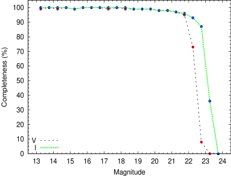
Figure 2: Completeness levels for the $V$ and $I$ bands as a function of magnitude derived from an artificial star experiment (ADDSTAR, see Sect. 2.2).

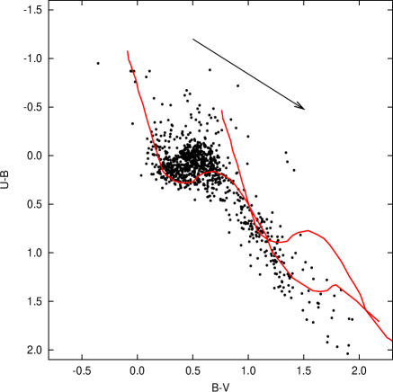
Figure 3: $(U-B)/(B-V)$ two color diagram for all the stars lying in the region with $V<16$ mag. The two continuous curves represent the ZAMS by Schmidt-Kaler (1982) shifted for the minimum ($E(B-V)$ = 0.25, left) and maximum ($E(B-V)$ = 1.1, right) reddening values. The reddening vector with a slope of 0.72 and size of $A_{v}$ = 3 mag is also shown.

2.3 Spectroscopy

For a set of 15 X-ray sources identified using XMM-Newton observations in the CrW field (see Claeskens et al., 2011), we obtained their optical spectra between 4 and 6 March 2003 using the EMMI instrument mounted on the ESO 3.5 m New Technology Telescope (NTT) at La Silla (PI: E. Gosset). This instrument was used in the Red Imaging and Low Dispersion Spectroscopy (RILD) mode with grism $\#5$ (wavelength range 4000 - 8700 Å). One spectrum was obtained with the VLT + FORS1 (see Claeskens et al., 2011). The data were reduced in the standard way using the long context of the ESO-MIDAS (European Southern Observatory Munich Image Data Analysis System) package. Since the observing conditions were favorable during our run, target spectra were calibrated using the flux spectrum of the standard star LTT 2415 (Hamuy et al., 1992).

2.4 Archival data: 2MASS

We used the 2MASS Point Source Catalog (PSC) (Cutri et al., 2003) for NIR ($JHK_{s}$) photometry of point sources in the CrW region. This catalog is said to be 99$\%$ complete up to the limiting magnitudes of 15.8, 15.1 and 14.3 in the $J$ (1.24$\mu$m), $H$ (1.66$\mu$m), and $K_{s}$ (2.16$\mu$m) bands, respectively. We selected only those sources that have NIR photometric accuracy $<$ 0.2 mag and detection in at least the $K_{s}$ and $H$ bands. Since the seeing ($\sim$FWHM of the stars intensity profile) for the WFI observations was around 1 arcsec, the optical counterparts of the 2MASS sources were searched using a matching radius of 1 arcsec.

3 Basic parameters

3.1 Reddening

The $(U-B)/(B-V)$ two-color diagram (TCD) was used to estimate the extinction toward the CrW region. In Fig. 3, we show the TCD with the zero-age-main-sequence (ZAMS) from Schmidt-Kaler (1982) shifted along the reddening vector with a slope of $E(U-B)/E(B-V)$ = 0.72 to match the observations. This shift will give the extinction directly toward the observed CrW region. The distribution of stars shows a wide spread in the diagram along the reddening line indicating the clumpy nature of the molecular cloud associated with this star-forming region. If we look at the MIR image of CrW (for detail see Sect. 5 and Fig. 16), we see the dark dust lane along with several enhancements of nebular materials at many places that are likely to be responsible for this spread in reddening. Figure 3 yields a minimum reddening value $E(B-V)$ of 0.25 with a wide spread leading to values up to 1.1 mag. Recent works (see Table 1) also indicate a spread in the value of $E(B-V)$ ($\sim$0.3 $-$ 0.8 mag) toward the $\eta$ Carinae region. Smith & Brooks (2008) suggest that a detailed optical study of the Carina nebula can easily be done since our sight line toward this nebula suffers little extinction and reddening compared to most of the massive star-forming regions. This seems true for the line of sight up to the first stars belonging to the complex, but it could perhaps not remain applicable to objects farther away and embedded inside the molecular cloud.

3.2 Reddening law

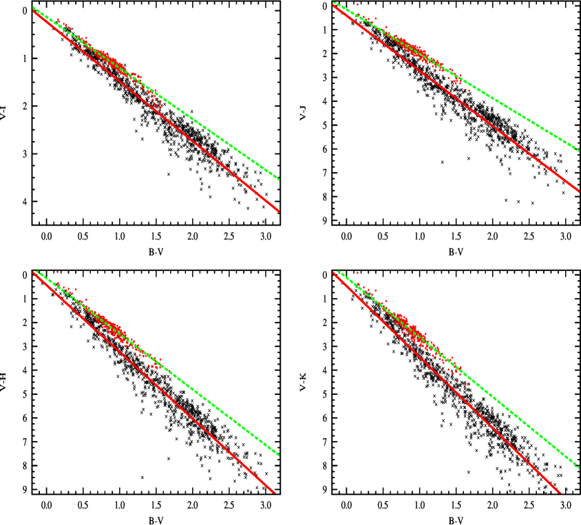
Figure 4: $(V-I),(V-J),(V-H)$, and $(V-K)$ versus $(B-V)$ TCDs for the stars in the CrW region ($r<10\arcmin$ from WR 22). The cross and dot symbols represent the stars with abnormal and normal reddening, respectively. Straight and dotted lines show least-squares fits to the data.

To study the nature of the gas and dust in young star-forming regions, it is very important to know the properties of the interstellar extinction and the ratio of total-to-selective extinction, i.e., $R_{V}=A_{V}/E(B-V)$. The normal reddening law for the solar neighborhood has been estimated to be $R_{V}$ = 3.1 $\pm$ 0.2 (cf. Guetter & Vrba, 1989; Whittet, 2003; Lim et al., 2011) but in the case of the $\eta$ Carinae region, there are several studies that claim that $R_{V}$ is anomalously high (see Feinstein et al., 1973; Herbst, 1976; Forte, 1978; Thé et al., 1980; Smith, 1987, 2002; Tapia et al., 1988; Vazquez et al., 1996). Recently, using 141 early type members in this region, Hur et al. (2012) derived an abnormal total-to-selective extinction ratio $R_{V}$ = 4.4 $\pm$ 0.04.

Table 1: Extinction, distance, and reddening values for the Carina region collected from the literature.

Region/cluster	$E(B-V)$	$R_{V}$	$M_{0}-M{{}_{V}}$	d(kpc)	References	Method/techniques
WR 22 (CrW)	0.36	3.1	12.15	2.7	Gosset et al. (2009)	–
Trumpler 14	–	–	11.1	–	Becker & Fenkart (1971)	–
	0.5	–	11.5	2.0	Thé & Vleeming (1971)	–
	–	–	12.7 $\pm$ 0.2	3.5	Walborn (1973)	Spectroscopic parallax
	–	3.2	12.7 $\pm$ 0.1	–	Humphreys (1978)	–
	–	–	–	2.8	Thé et al. (1980)	–
	–	–	12.3 $\pm$ 0.1	–	Walborn (1982)	–
	0.55 $\pm$ 0.08	–	12.2 $\pm$ 0.2	–	Feinstein (1983)	–
	–	3.2	12.7 $\pm$ 0.1	3.5	Morrell et al. (1988)	Spectroscopic parallax
	–	–	12.3 $\pm$ 0.1	2.8	Morrell et al. (1988)	Spectroscopic parallax
	0.82 $\pm$ 0.12	–	11.9 $\pm$ 0.2	2.4 $\pm$ 0.3	Tapia et al. (1988)	Main-sequence fitting
	–	3.2	12.8 $\pm$ 0.2	–	Massey & Johnson (1993)	Spectroscopic parallax
	0.57 $\pm$ 0.13	4.7 $\pm$ 0.7	12.5 $\pm$ 0.2	3.1 $\pm$ 0.3	Vazquez et al. (1996)	Main-sequence fitting
	0.58	3.2	12.8 $\pm$ 0.1	–	DeGioia-Eastwood et al. (2001)	Spectroscopic parallax
	–	–	12.2 $\pm$ 0.7	–	Tapia et al. (2003)	Spectroscopic parallax
	0.57 $\pm$ 0.12	4.2 $\pm$ 0.2	12.0 $\pm$ 0.2	2.5 $\pm$ 0.3	Carraro et al. (2004)	Main-sequence fitting
	0.36 $\pm$ 0.04	4.4 $\pm$ 0.2	12.3 $\pm$ 0.2	2.9 $\pm$ 0.3	Hur et al. (2012)	Proper motion
Trumpler 15	–	–	11.1	–	Becker & Fenkart (1971)	–
	0.4	–	11.5	1.6	Thé & Vleeming (1971)	–
	–	–	12.9	3.7	Walborn (1973)	Spectroscopic parallax
	–	–	12.9	–	Humphreys (1978)	–
	–	–	–	2.5	Thé et al. (1980)	–
	–	3.2	11.8 $\pm$ 0.1	2.3	Morrell et al. (1988)	Spectroscopic parallax
	–	–	12.1 $\pm$ 0.3	2.6	Morrell et al. (1988)	Spectroscopic parallax
	0.49$\pm$ 0.09	–	12.1 $\pm$ 0.2	2.6 $\pm$ 0.3	Tapia et al. (1988)	Main-sequence fitting
	0.49$\pm$ 0.09	–	12.1 $\pm$ 0.2	2.9	Tapia et al. (2003)	Spectroscopic parallax
	–	–	12.3 $\pm$ 0.2	–	Carraro et al. (2004)	Main-sequence fitting
Trumpler 16	0.44	–	11.9	2.5	Thé & Vleeming (1971)	–
	0.4	–	12.1	2.7	Feinstein et al. (1973)	–
	–	3.0	12.1 $\pm$ 0.2	2.6	Walborn (1973)	Spectroscopic parallax
	–	–	12.2 $\pm$ 0.1	–	Humphreys (1978)	–
	–	–	12.0	2.8	Thé et al. (1980)	–
	–	3.1	11.8 $\pm$ 0.1	2.3	Levato & Malaroda (1982)	Spectroscopic parallax
	–	–	12.3 $\pm$ 0.1	–	Walborn (1982)	–
	0.68 $\pm$ 0.15	–	12.0 $\pm$ 0.2	2.5 $\pm$ 0.2	Tapia et al. (1988)	Main-sequence fitting
	–	–	12.5 $\pm$ 0.1	–	Massey & Johnson (1993)	Spectroscopic parallax
	0.58	3.2	12.8 $\pm$ 0.1	–	DeGioia-Eastwood et al. (2001)	Spectroscopic parallax
	–	–	12.0 $\pm$ 0.6	2.5	Tapia et al. (2003)	Spectroscopic parallax
	0.61 $\pm$ 0.15	3.5 $\pm$ 0.3	13.0 $\pm$ 0.3	3.9 $\pm$ 0.5	Carraro et al. (2004)	Main-sequence fitting
	0.36 $\pm$ 0.04	4.4 $\pm$ 0.2	12.3 $\pm$ 0.2	2.9 $\pm$ 0.3	Hur et al. (2012)	Proper motion
Collinder 228	–	–	12.0 $\pm$ 0.2	2.5	Feinstein et al. (1973)	–
	–	–	12.2	–	Walborn (1973)	Spectroscopic parallax
	–	–	12.0 $\pm$ 0.3	–	Humphreys (1978)	–
	–	3.2	–	2.5	Thé et al. (1980)	–
	–	–	12.06	2.6	Levato & Malaroda (1981)	Spectroscopy
	0.64 $\pm$ 0.26	–	11.6 $\pm$ 0.4	2.1 $\pm$ 0.4	Tapia et al. (1988)	Main-sequence fitting
	–	–	–	1.9 $\pm$ 0.2	Carraro & Patat (2001)	–
Collinder 232	0.68 $\pm$ 0.21	–	12.0 $\pm$ 0.2	2.5 $\pm$ 0.2	Tapia et al. (1988)	Main-sequence fitting
	0.48 $\pm$ 0.12	3.7$\pm$ 0.03	11.8 $\pm$ 0.2	2.3 $\pm$ 0.3	Carraro et al. (2004)	Main-sequence fitting
Bochum 9	0.63 $\pm$ 0.08	–	–	4.7	Patat & Carraro (2001)	–
Bochum 10	–	–	12.8	–	Feinstein (1981)	–
	–	–	12.2	–	Fitzgerald & Mehta (1987)	–
	0.48 $\pm$ 0.05	–	12.2	2.7	Patat & Carraro (2001)	–
NGC 3324	–	–	12.5 $\pm$ 0.2	–	Clariá (1977)	–
	–	–	12.4 $\pm$ 0.03	3.0 $\pm$ 0.1	Carraro & Patat (2001)	–
Trumpler 14,	–	3.2 $\pm$ 0.3	12.2	2.7 $\pm$ 0.2	Turner et al. (1980)	–
15, 16 and Cr 228

We used the TCDs as described by Pandey et al. (2003) to study the nature of the extinction law in the CrW region. The TCDs of the form of $(V-\lambda)$ versus $(B-V)$, where $\lambda$ indicates one of the wavelengths of the broad-band filters ($R,I,J,H,K,L$), provide an effective method for distinguishing the influence of the normal extinction produced by the diffuse interstellar medium from that of the abnormal extinction arising within regions having a peculiar distribution of dust sizes (cf. Chini & Wargau, 1990; Pandey et al., 2000).

We clearly see in Fig. 4 that there are two types of distribution having different slopes. We selected all the stars belonging to these two populations and plotted their $(V-I),(V-J),(V-H)$ and $(V-K)$ vs. $(B-V)$ TCDs in Fig. 4. The respective slopes relating these colors were found, for the red-dot stars, to be $1.07\pm 0.02,1.86\pm 0.02,2.33\pm 0.03$, and $2.50\pm 0.03$, which are approximately equivalent to the normal galactic values, i.e., 1.10, 1.96, 2.42, and 2.60, respectively. The objects with black crosses display steeper slopes, i.e., $1.28\pm 0.01,2.34\pm 0.03,2.84\pm 0.03$ and $3.03\pm 0.03$ for $(V-I),(V-J),(V-H)$ and $(V-K)$ vs. $(B-V)$, respectively. If we plot the spatial distribution of the red dots and black crosses, we clearly see that all the red dots are uniformly distributed, whereas all the black crosses are distributed away from the obscured region of the molecular cloud. It means that the black crosses are most probably background stars, and their light is seen through the molecular cloud (see Preibisch et al., 2011a; Roccatagliata et al., 2013, and references therein). Therefore, the ratios [$E(V-\lambda)$]/[$E(B-V)$] ($\lambda$ $\geq$ $\lambda_{I}$) for the stars in the background yield a high value for $R_{V}$ ($\sim$3.7 $\pm$ 0.1), indicating an abnormal grain size in the observed region. Many investigators (see column 3 of Table 1) have also found evidence of larger dust grains in the Carina region. Marraco et al. (1993) have found that the value of $\lambda_{max}$ (the wavelength at which maximum polarization occurred, which is also an indicator of the mean dust grain size distribution) is higher than the canonical value for the general diffuse ISM.

Several studies have already pointed toward an anomalous reddening law with a high $R_{V}$ value in the vicinity of star-forming regions (see, e.g., Pandey et al., 2003). However, for the Galactic diffuse interstellar medium, a normal value of $R_{V}$ = 3.1 is well accepted. The higher-than-normal value of $R_{V}$ has usually been attributed to the presence of larger dust grains. There is evidence that, within the dark clouds, accretion of ice mantles on grains and coagulation due to colliding grains change the size distribution towards larger particles. On the other hand, in star-forming regions, radiation from massive stars may evaporate ice mantles resulting in small particles. Here, it is interesting to mention that Okada et al. (2003) suggest that efficient dust destruction is undergoing in the ionized region on the basis of the [Si II] 35 to [N II] 122 $\mu$m ratio. Chini & Kruegel (1983) and Chini & Wargau (1990) have shown that both larger and smaller grains may increase the ratio of total-to-selective extinction.

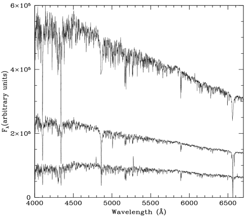
Figure 5: Flux-calibrated spectra of the O-A-F-G type stars in our spectroscopic sample of the CrW region. The spectra have been randomly shifted vertically for clarity. The spectral types become progressively later from left to right and from top to bottom.

3.3 Distance

The Carina nebula is a very large (angular size $>$ $2^{\circ}\times 1.5^{\circ}$) active star-forming region containing a number of young star clusters featuring very massive O-type stars. Recently many authors have considered that the distance to $\eta$ Carinae and to the whole Carina region is 2.3 kpc (see, e.g., Smith, 2006b; Povich et al., 2011). There is a large discrepancy in the measured distances to the clusters situated within this nebula, as can be seen from Table 1. This large scatter in the distance occurs because, as noted by Smith & Brooks (2008), the direction of the Galactic plane in the Carina nebula nearly looks down the tangent point of the Sagittarius-Carina spiral arm. The two clusters Tr 14 and Tr 16, located towards the center of the Carina nebula, have been extensively studied by several authors, but the debate about their distance is still open. Vazquez et al. (1996) estimated a distance modulus of $V_{0}-M_{V}$ = 12.5 $\pm$ 0.2 mag for Tr 14. By applying an abnormal reddening law, Tapia et al. (2003) derived $V_{0}-M_{V}$ = 12.1 mag. In their study, they adopted $A_{V}$ = 1.39$E(V-J)$ and found that both clusters are situated at the same distance. But in another study, Carraro et al. (2004) concluded that both clusters are situated at different distances with $V_{0}-M_{V}$ = 12.3 $\pm$ 0.2 mag for Tr 14 and 13.0 $\pm$ 0.3 mag for Tr 16. Recently, Hur et al. (2012) concluded that Tr 14 and Tr 16 are at the same distance within the observational errors ($V_{0}-M_{V}$ = 12.3 $\pm$ 0.2 mag, i.e., d = 2.9 $\pm$ 0.3 kpc). Their derived distance is based upon the proper motion, which is comparatively more accurate than other methods. Since we are concentrating on the western side of the Carina nebula containing some part of Tr 14, for the present study, we have adopted a distance of 2.9 kpc for CrW as given by Hur et al. (2012).

4 Results

4.1 Spectroscopically identified sources

The MK spectral types of 15 X-ray emitting sources in the CrW region were established using the newly acquired spectra (see Sect. 2.3) and their comparison with the digital spectral classification atlas compiled by R.O. Gray and available on the web. The results are summarized in Table 2, from which we may infer that the majority of identified sources are late-type stars (see Fig. 5 for different spectral types), and none of these stars features an $H\alpha$ emission.

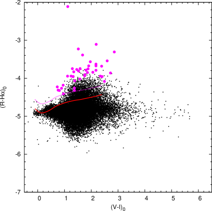
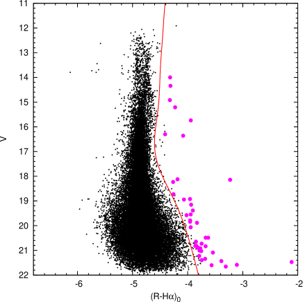
Figure 6: Left panel: The $(R-H\alpha)_{0}$ index is shown as a function of the $(V-I)_{0}$ color. The solid line indicates the relation for MS stars as taken from Sung et al. (1997). The dashed line (magenta) yields the thresholds for $H\alpha$ emitter candidates. Right panel: $V$ versus $(R-H\alpha)_{0}$ CMD. The magenta circles represent $H\alpha$ emitter candidates. An envelope as discussed in Sect. 4.2.1 is indicated by a solid line.

Three X-ray sources (i.e. #6, #9, and #20; in Table 2) belong to spectral type O, of which #6 and #9 are correlated with HD 92607 and HD 92644, respectively. Houk & Cowley (1975) classify them as O type stars (HD 92607 – O9 II/III and HD 92644 – O9.5/B0III). Our present analysis rather favors spectral types of O8.5 III for #6 and O9.7 V for #9. These results broadly confirm previous classifications of these sources (see also Claeskens et al., 2011). The X-ray properties of both stars are discussed in detail by Claeskens et al. (2011, see their discussion and notes on individual objects). They find that the observed X-ray count rate for #9 is 3.8 times lower than #6, but both are quite soft. Star #20 is identified as a reddened O7 star with observed $V$ = 13.03 and $(B-V)$ = 1.83 mag (cf. Table 2).

The remaining 12 sources have counterparts that are classified as late-type stars: three are of spectral type A, three are F stars, and six are classified as G-type stars. Stars #11, #19, and #37 are identified as A5 V, A1 III, and A1 V, respectively. Similarly #3, #10, and #23 belong to F5 V, F8 V, and F3 V spectral types, respectively. Claeskens et al. (2011) in their study found that source #18 is among the brightest X-ray sources in this field; however, they could not identify any optical counterpart for this object from the GSC2.2 catalog. Based on IR colors, they computed the $V$ band magnitude of this object to be in between 20.2 $-$ 21.5. Later on by visual inspection of Digital Sky Survey images, they found a star having brightness 18 $-$ 19 at the exact source location. We also found a star with magnitude 18.214 $\pm$ 0.012 (cf. Table 2, column 4) at a similar position. Binarity could explain why this star is brighter in the optical than expected from its near-IR magnitudes (Claeskens et al., 2011). It could reside in front of the Carina, but it could also be intrinsically brighter than a main-sequence (MS) star. Sources #7, #12, #15, #32, #40, and #42 are characterized as G6 III, G9 V, G8 III, G3 V-III, G8 V, and G9 III spectral type, respectively. Based on the observed X-ray counts, Claeskens et al. (2011) claim that #42 is a variable star. It is also worthwhile to mention that two sources (#7 and #15) are identified as PMS sources (see Table 2) in the present study (cf. Sect. 4.2.3).

4.2 YSOs identification

The PMS stars (YSOs) are mainly grouped into the classes 0-I-II-III, which represent in-falling protostars, evolved protostars, classical T-Tauri stars (CTTSs), and weak line T Tauri stars (WTTSs), respectively (cf. Feigelson & Montmerle, 1999). Class 0 & I YSOs are so deeply buried inside the molecular clouds that they are not visible at optical wavelengths. The CTTSs feature disks from which the material is accreted, and emission in $H\alpha$ can be seen as due to this accreting material. These disks can also be probed through their IR excess (compared to normal stellar photospheres). WTTSs, on the contrary, have little or no disk material left, hence have no strong $H\alpha$ emission and IR excess. It is evident from the recent studies that the X-ray luminosity from WTTSs is significantly higher than for the CTTSs with circumstellar disks or protostars with accreting envelopes (Stassun et al., 2004; Telleschi et al., 2007; Prisinzano et al., 2008). In this section we report the tentative identification of YSOs on the basis of their $H\alpha$ emission, IR excess, and X-ray emission.

4.2.1 On the basis of $H\alpha$ emission

The stars showing emission in $H\alpha$ might be considered as PMS stars or candidates, and the strength of the $H\alpha$ line (measured by its equivalent width ‘EW($H\alpha$)’) is a direct indicator of their evolutionary stage. The conventional distinction between CTTSs and WTTSs is an EW($H\alpha$) $>10\AA$ for the former (see Herbig & Bell, 1988). However, Bertout (1989) has suggested that a limiting value of 5$\AA$ might be more appropriate. More recently, investigators have tied the definition to the shape (width) of the $H\alpha$ line profile (see White & Basri, 2003; Jayawardhana et al., 2003). In the study of NGC 6383, Rauw et al. (2010) find that an $H\alpha$ equivalent width of 10$\AA$ corresponds to an $(R-H\alpha)$ index of 0.24 $\pm$ 0.04 above the MS relation of Sung et al. (1997). They have further used this as a selection criterion for identifying $H\alpha$ emitters. In our study, we have considered a source as probable $H\alpha$ emitter only if the $(R-H\alpha)$ index is 0.24 above the MS relation by Sung et al. (1997).

The $H\alpha$ filter at WFI has a special passband, therefore it cannot be directly linked to any existing standard photometric system (see also Rauw et al., 2010). By selecting ten stars observed with EMMI (see Sect. 2.3), whose spectra do not exhibit $H\alpha$ emission, we calibrated the zero point by comparing the observed $R-H\alpha$ and dereddened $(V-I)$ with the $(R-H\alpha)_{0}$ versus the $(V-I)_{0}$ relation of emission free MS stars as determined by Sung et al. (1997) for NGC 2264. The $(V-I)$ color is dereddened by $E(V-I)$ value of $E(B-V)_{min}$ $\times$ 1.5. In Fig. 6, we plotted the $(R-H\alpha)_{0}$ vs. $(V-I)_{0}$ distribution of all the stars along with the MS given by Sung et al. (1997).

Since there is large scatter in the distribution (cf. Fig. 6; left panel), there may be false identifications of $H\alpha$ emitters. To minimize this, we introduced another selection criterion to identify the $H\alpha$ emitters in addition to the previous one. We used the $V$ vs. $(R-H\alpha)_{0}$ color magnitude diagram (CMD) (cf. Fig. 6; right panel) and defined an envelope that contains most of the stars following the MS. The stars that have a value of $(R-H\alpha)_{0}-\sigma_{(R-H\alpha)}$ greater than that of the envelope of the MS can be assumed to be probable $H\alpha$ emitters. In our study, we therefore consider that a star is a good $H\alpha$ emission candidate if it satisfies both conditions. We have identified 41 YSOs in our study as potential $H\alpha$ emitters, and these can be seen in Fig. 16.

4.2.2 On the basis of IR excess

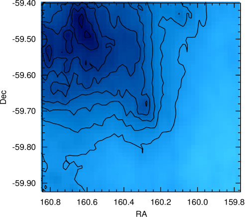
Figure 7: Column density distribution of the molecular cloud in our field of view, as derived from the near-infrared reddening of stars. The lowest contour corresponds to $A_{v}$ = 3.4, the step size of the contours is 0.2.

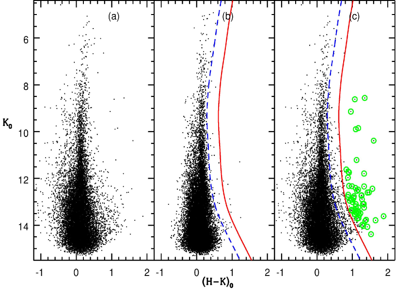
Figure 8: $K{{}_{0}}/(H-K){{}_{0}}$ CMD for (a) stars in the CrW region, (b) stars in the field region and (c) same stars as in panel (a) along with identified probable NIR-excess stars. The blue dashed line represents the envelope of field CMD, whereas the red solid line demarcates the distribution of IR excess sources from MS stars.

Recently Gaczkowski et al. (2013) have obtained Herschel PACS and FIR maps that cover the full area of the CNC and reveal the population of deeply embedded YSOs, most of which are not yet visible at the MIR or NIR wavelengths. They studied the properties of the 642 objects that are independently detected as point-like sources in at least two of the five Herschel bands. For those objects that can be identified with apparently single Spitzer counterparts, they used radiative transfer models to derive information about the basic stellar and circumstellar parameters. They found that about 75% of the Herschel-detected YSOs are Class 0 protostars and that their masses (estimated from the radiative transfer modeling) range from $\sim$1 M_⊙ to $\sim$10 M_⊙. Out of these 642 sources, 105 fall in our studied region.

Using NIR/MIR data of 2MASS and Spitzer, Povich et al. (2011) present a catalog of 1439 YSOs spanning a 1.42 deg² field surveyed by the Chandra Carina Complex Project (CCCP) (for more details about CCCP see Townsley et al., 2011). This field includes the major ionizing clusters and the most active sites of ongoing star formation within the Great Nebula in Carina. YSO candidates were identified via IR excess emission from dusty circumstellar disks and envelopes, using data from the Spitzer Space Telescope (the Vela–Carina survey) and the 2MASS database. They model the 1-24 $\mu$m IR spectral energy distributions of the YSOs to constrain their physical properties. Their Pan-Carina YSO Catalog (PCYC) is dominated by intermediate-mass (2 M_⊙ $<$ M $\leq$ 10 M_⊙) objects with disks, including Herbig Ae/Be stars and their less evolved progenitors. Out of these 1439 sources, 136 fall in our studied region.

Recently, Preibisch et al. (2011b) used HAWK-I at the ESO VLT to produce a deep and wide NIR survey that is deep enough to detect the full low-mass stellar population (i.e. down to $\sim$0.1M_⊙ and for extinctions up to $A_{V}\sim$15 mag) in all the important parts of the CNC, including the clusters Tr 14, 15, and 16, as well as the South Pillars region. They analyzed CMDs to derive information about the ages and masses of the low-mass stars. Unfortunately, their surveyed region does not cover our studied region. Therefore for the present study we used NIR data from the 2MASS survey to identify sources with IR excess. We used the following scheme to make the distinction between the sources with IR excess and those that are simply reddened by dust along the line of sight (Gutermuth et al., 2005). First we measure the line of sight extinction to each source as parameterized by the $E_{H-K}$ color excess due to the dust present along the lines of sight. For objects where we have $J$ photometry in addition to $H$ and $K_{s}$ with the condition that they are positioned above the extension of CTTSs locus and have color $[J-H]\geq 0.6$, we used the equations given by Gutermuth et al. (2009) to derive the adopted intrinsic colors. The difference between the intrinsic color and the observed one will give the extinction value. Once we had the extinction value for the stars, we generated an extinction map for the whole CrW region. The extinction values in a sky plane were calculated with a resolution of 5 arcsec by taking the mean of extinction value of stars in a box having a size of 17 arcsec. The resulting extinction map, smoothed to a resolution of 0.6 arcmin, is shown in Fig. 7. This IR extinction map represents the column density distribution of the molecular cloud associated with the CrW region. We can clearly see the high density region toward the northeast of CrW and then the density following the dust lane as visible in the 4.6 $\mu$m image (cf. Sect. 5, see Fig. 16). Thanks to less extinction, longer wavelength observations can penetrate deeper inside the nebulosity than do shorter wavelengths. For this reason, there are many stars in the CrW region that do not have $J$ band photometry. Once we constructed the extinction map, we used this to also deredden the stars having no $J$ band detection. Here it is worthwhile to note that we used CTTSs loci to estimate reddening by back-tracing all the stars located above the CTTSs loci or its extension to the CTTSs loci or its extension. It is quite probable that the genuine CTTSs are mixed with deeply embedded MS stars that could fall above the CTTSs locus in the 2MASS color-color diagram. Therefore, when we deredden this mixed sample of stars, the reddening value for CTTSs will get overestimated because of their surrounding cocoon of dust/gas, whereas for the MS stars, it will get underestimated because the intrinsic color of MS stars lies below CTTSs loci.

In Fig. 8, we have plotted the dereddened NIR CMDs, $K_{0}$ versus $(H-K)_{0}$, for the CrW region and the nearby reference field region having same area as CrW. Since both the field and CrW region CMDs are dereddened by the same technique, the underestimation/overestimation of the $A_{v}$ value will not affect our analysis much. However, owing to the clumpy nature of the molecular cloud associated with the CrW region, the dereddened CMD for CrW will show more scatter than the field CMD. A comparison with the reference field CMD reveals that there might be many stars showing excess emission that is apparent from their distribution at $(H-K)_{0}\lesssim 0.6$ mag. Therefore, we defined an envelope representing a cut-off line (Figs. 8b,c) on the basis of the CMD of the CrW region and of the field one. We then designed an additional envelope (solid line in red) shifted to the red from the preceding one by an amount corresponding to $A_{v}$ = 5 (to compensate for the scattering due to the clumpy nature of molecular clouds). Doing that, we aim at isolating probable NIR excess stars from reddened MS stars. Since we know that the photometric error is larger at the fainter end of the CMD, the shape of the cut-off line at the fainter end is adjusted accordingly. All the stars having a color ‘$(H-K)_{0}-\sigma_{(H-K)_{0}}$’ greater than the red cut-off line might have an excess emission in the $K$ band and thus can reasonably be considered to be probable YSOs (see also Mallick et al., 2012). While this sample is dominated by YSOs, it may also contain the following types of contaminations: variable stars, dusty asymptotic giant branch (AGB) stars, unresolved planetary nebulae, and background galaxies (Robitaille et al., 2008; Povich et al., 2011). We used the CMD of the reference field covering the same area as the CrW region to calculate the fraction of contaminating objects in our sample. The reference field was around 1.5^∘ westward from the center of the CrW (cf. Fig. 1).

The number of probable NIR excess stars in the reference field is about 8 whereas the number of probable NIR excess stars in the CrW region is 60. This means that we have a contamination of about 13% in our sample. The majority of these probable NIR excess stars follow the high density region in the CrW region (see Fig. 16) and may be deeply embedded in that nebulosity. Povich et al. (2011) have identified many YSOs that are mainly in the irradiated surface of the cloud (see Fig. 16) but recently, based on Herschel FIR data, Gaczkowski et al. (2013) have identified YSOs that are also located within the dark lane of the CrW region.

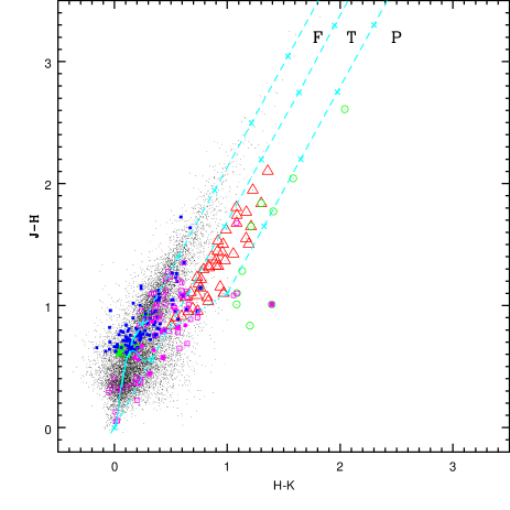
Figure 9: $(J-H)/(H-K)$ color-color diagram of sources detected in the $JHKs$ bands in the CrW region. The sequences of dwarfs (solid curve) and giants (thick dashed curve) are from Bessell & Brett (1988). The dotted line represents the locus of T Tauri stars (Meyer et al., 1997). Parallel dashed straight lines represent the reddening vectors (Cohen et al., 1981). The crosses on the dashed lines are separated by $A_{V}$ = 5 mag. YSOs are also shown. Open magenta squares = Spitzer; filled magenta circles = $H\alpha$; filled squares = X-ray emitting WTTSs (green = XMM-Newton, blue = Chandra); open red triangles = CTTSs and open green circles = probable NIR-excess sources (see text for the classification scheme).

YSOs such as CTTSs, WTTSs, and Herbig Ae/Be stars tend to occupy different regions on the NIR TCDs. In Fig. 9, we have plotted the NIR TCD using the 2MASS data for all the sources lying in the observed region. All the 2MASS magnitudes and colors were converted into the California Institute of Technology (CIT) system. All the curves and lines are also in the CIT system. The shown reddening vectors are drawn from the tip (spectral type M4) of the giant branch (“upper reddening line”), from the base (spectral type A0) of the MS branch (“middle reddening line”) and from the tip of the intrinsic CTTSs line (“lower reddening line”). The extinction ratios $A_{J}/A_{V}=0.265,A_{H}/A_{V}=0.155$ and $A_{K}/A_{V}=0.090$ have been taken from Cohen et al. (1981). We classified the sources according to three regions in this diagram (cf. Ojha et al., 2004). The ‘F’ sources are located between the upper and middle reddening lines and are considered to be either field stars (MS stars, giants) or Class III and Class II sources with small NIR-excess. ‘T’ sources are located between the middle and lower reddening lines. These sources are considered to be mostly CTTSs (or Class II objects) with large NIR-excess. There may be an overlap of Herbig Ae/Be stars in the ‘T’ region (Hillenbrand et al., 1992). ‘P’ sources are those located in the region redward of the lower reddening line and are most likely Class 0/I objects (protostellar-like objects; Ojha et al. (2004)). It is worthwhile also mentioning that Robitaille et al. (2006) show that there is a significant overlap between protostars and CTTSs. The NIR TCD of the observed region (Fig. 9) indicates that a significant number of sources that have previously been identified as probable NIR-excess stars lie in the ‘T’ region. Forty-one sources have been designated as CTTSs in our study with the condition that they fall in the ‘T’ region of the NIR TCD (Fig. 9) and are redward of the dashed blue cut-off line in the dereddened CMD (Fig. 8). We also have plotted probable NIR excess sources that are detected in ‘$J$’ band (10 out of 60). Most of these sources are located in the ‘P’ region in Fig. 9, which means that they are most likely Class 0/I objects.

4.2.3 On the basis of X-ray emission

The NIR-excess-selected YSO candidate samples are generally considered incomplete because the NIR-excess emission in young stars disappears on timescales of just a few Myr (see Briceño et al., 2007). At an age of $\sim$3 Myr, only $\sim$50% of the young stars still show NIR excesses, and by $\sim$5 Myr this fraction is reduced to $\sim$15% (Preibisch et al., 2011c). Since the expected ages of most young stars in the CNC are several Myr, any IR-excess-selected YSO sample will be highly incomplete. To tackle this problem, we used the X-ray emitting point sources in the region to identify YSO candidates. The X-ray detection methods are sensitive to young stars that have already dispersed their circumstellar disks, thus avoiding the bias introduced when selecting samples only based on IR excess (Preibisch et al., 2011c).

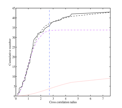
Figure 10: Cumulative numbers of correlations between the X-ray detected sources and the WFI catalog. The thick curve represents the observed numbers, the dashed curve shows the best fit, and the dot-dashed line (magenta) and dotted (red) curves correspond to the numbers of real and spurious sources, respectively. The vertical line indicates the optimal correlation radius r_c.

XMM-Newton observations

The XMM-Newton satellite has observed the CrW region in the course of the study of the massive binary WR 22. The corresponding results have been presented in separate papers (see Gosset et al., 2009; Claeskens et al., 2011). In this section we cross-correlated the sources detected in our photometric data of the CrW region with the positions of 43 X-ray sources from Claeskens et al. (2011). The positions of the X-ray sources as given by Claeskens et al. (2011, columns 8 and 9 of their table 2) refer to the astrometric frame as determined from the XMM-Newton on-board Attitude and Orbit Control System. The cross-correlation with the GSC and the present optical catalog suggests making a small correction. We therefore suggest decreasing the right ascension of Claeskens et al. (2011) by 0$\aas@@fstack{\prime\prime}$25 and increasing the declination by 0$\aas@@fstack{\prime\prime}$96. No rotation was detected. We adopt these new positions for the 43 X-ray sources.

We defined an optimal cross-correlation radius to find a compromise between correlations missed due to astrometric errors and spurious associations in the CrW field. To derive the optimal correlation radius, we applied the technique of Jeffries et al. (1997). In this method, the distribution of the cumulative number of cataloged sources as a function of the cross-correlation radius $r_{c}$ is given by

$$\Phi(d\leq r_{c}) = A\,\left[1-\exp{\left(\frac{-r_{c}^{2}}{2\,\sigma^{2}}\right)}\right]$$

$$+ (N-A)\,\left[1-\exp(-\pi\,B\,r_{c}^{2})\right].$$

In this equation $N$, $A$, $\sigma$, and $B$ represent the total number of cross-correlated X-ray sources ($N=43$), the number of true correlations, the uncertainty in the X-ray source position, and the surface density of the catalog of photometric sources, respectively. In the course of fitting the integrated number of correlations with the CrW photometric catalog as a function of the separation (where 43 X-ray sources have an optical source located closer than 8 arcsec), we derived the fitting parameters as $A=33.78$, $\sigma=0.9$ arcsec, and $B=2.3\times 10^{-2}$ arcsec^-2 (see Fig. 10). The optimal correlation radius was chosen to be $r_{c}$ = 2.7$\,\arcsec$, which implies that there is no more than one spurious association among the 34 correlations; i.e., the optical counterparts of 79% of the XMM-Newton sources in the CrW field should thus be reliably identified.

Claeskens et al. (2011) also cross-correlated these X-ray sources ($N=43$), but they searched the optical counterparts using the Guide Star Catalog version 2.2 (GSC2.2). Their fitting parameters are $A=35.4$, $B=2\times 10^{-3}$ arcsec^-2, and $\sigma=1.8$ arcsec. The number of true correlations ($A$) of both studies are very much consistent. The surface density ($B$) of the catalog of optical sources in the present study is an order of magnitude higher than in Claeskens et al. (2011), while our $\sigma$ value is half that of these authors. The results of the cross-identification are listed in Table 2. When several optical counterparts are present, only the closest one is given. The first column is the ID of the X-ray sources from Claeskens et al. (2011). Columns 2 and 3 are their respective RA and Dec in degree (from our photometric catalog). In the next columns the $V$ magnitude, colors $(V-I)$, $(V-R)$, $(B-V)$ and $(U-B)$ are reported. Sources with a spectral classification are mentioned in the next-to-last column.

Table 2: Cross-identification of 43 X-ray sources from Claeskens et al. (2011) with CrW optical photometry. Stars brighter than $V$ = 11.3 are from the literature. The YSOs identified in Section 4.2 are also mentioned in the last column.

ID(X-ray)	$\alpha$(J2000)	$\delta$(J2000)	$V$	$(V-I)$	$(V-R)$	$(B-V)$	$(U-B)$	Spectral type	YSO number†
#1	159.894496	-59.737510	20.386	2.860	1.438	2.250	N/A	–	183
#2	159.947016	-59.608981	12.991	0.809	0.436	0.653	-0.042	–	–
#3	159.948029	-59.746218	10.470	N/A	N/A	0.440	N/A	F5 V	–
#4	159.983333	-59.618056	11.279	N/A	N/A	0.668	N/A	–	–
#5	160.042973	-59.619011	17.720	2.299	1.195	1.721	1.051	–	57
#6	160.051779	-59.802809	8.140	N/A	N/A	-0.020	-0.780	O8.5 III	–
#7	160.069977	-59.534346	14.720	1.386	0.787	1.006	0.673	G6 III	13
#8	–	–	–	–	–	–	–	–	–
#9	160.132138	-59.778854	8.880	N/A	N/A	-0.030	-0.900	O9.7 V	–
#10	160.161981	-59.462519	12.839	0.807	0.419	0.590	0.028	F8 V	–
#11	160.174252	-59.621872	12.609	0.429	0.258	0.320	0.108	A5 V	–
#12	160.174412	-59.539547	14.974	0.954	0.540	0.736	0.149	G9 V	–
#13	160.184003	-59.826372	17.565	3.222	1.551	2.103	1.018	–	–
#14	160.193248	-59.700809	19.680	2.144	1.115	1.544	N/A	–	–
#15	160.214424	-59.622191	15.365	1.332	0.716	1.109	0.609	G8 III	18
#16	–	–	–	–	–	–	–	–	–
#17	160.229239	-59.639602	17.422	1.552	0.835	1.217	0.607	–	48
#18	160.230446	-59.710999	18.214	1.586	0.928	1.086	0.373	F8 V	–
#19	160.235367	-59.862561	11.363	0.340	N/A	N/A	N/A	A1 III	–
#20	160.247070	-59.457005	13.031	1.825	0.860	1.340	-0.031	O7	–
#21	–	–	–	–	–	–	–	–	–
#22a	160.322983	-59.676915	6.420	N/A	N/A	0.080	-0.730	–	–
#23	160.335850	-59.589894	11.692	0.718	N/A	0.841	-0.285	F3 V	–
#24	160.338038	-59.659587	17.131	1.316	0.758	0.978	0.259	–	–
#25	–	–	–	–	–	–	–	–	–
#26	160.362639	-59.656561	16.698	1.334	0.774	0.896	0.494	–	–
#27	160.364564	-59.686933	16.339	1.174	0.658	0.903	0.215	–	–
#28	160.387108	-59.604288	19.416	2.737	1.136	1.667	N/A	–	–
#29	160.426017	-59.635431	16.982	1.335	0.712	1.054	0.482	–	–
#30	160.437963	-59.807270	19.050	2.058	0.922	1.818	N/A	–	–
#31	160.464076	-59.720771	12.626	0.782	0.442	0.550	-0.019	–	–
#32	160.478811	-59.689836	13.146	1.224	0.793	0.935	0.923	G3 V-III	–
#33	–	–	–	–	–	–	–	–	–
#34	–	–	–	–	–	–	–	–	–
#35	–	–	–	–	–	–	–	–	–
#36	–	–	–	–	–	–	–	–	–
#37	160.523400	-59.604232	14.022	0.554	0.316	0.357	0.158	A1 V	–
#38	160.556738	-59.599388	18.204	2.910	1.446	2.081	0.479	–	87
#39	160.564481	-59.565945	19.215	2.738	1.145	1.679	N/A	–	–
#40	160.603836	-59.669004	14.842	1.105	0.636	0.576	0.164	G8  V	–
#41	160.636112	-59.611374	16.242	1.834	0.975	1.461	1.079	–	30
#42	160.652591	-59.731771	15.372	1.454	0.764	1.096	0.746	G9  III	–
#43	160.679111	-59.591296	15.898	1.365	0.738	1.165	0.425	–	–

^a WR 22 itself; ^†The YSO entry numbers are from Table 3.

Chandra X-ray observations

Recently, a wide area (1.42 deg²) of the Carina complex has been mapped by the Chandra X-ray Observatory (CCCP, Townsley et al., 2011). These images were obtained with the Advanced CCD Imaging Spectrometer (ACIS; Garmire et al., 2003). This CCCP study mainly includes the data from the ACIS-I array, although ACIS-S array CCDs S2 and S3 were also operational during the observations. But most of the sources on S2 and S3 are crowded and dominated by the background in the CCCP data (Townsley et al., 2011). In this survey, 14369 X-ray sources were detected over the whole CCCP survey region. Out of these, the CrW region contains 1465 sources. Since the on-axis Chandra PSF is 0.5$\,\arcsec$ and because it degrades at large off-axis angles (see, e.g., Getman et al., 2005; Broos et al., 2010), we have taken an optimal matching radius of 1 arcsec to determine the optical/NIR counterparts of these X-ray sources. This size of the matching radius is well established in other studies as well (see, e.g., Feigelson et al., 2002; Wang et al., 2007). We identified 469 sources that have 2MASS NIR counterparts and fall in the CrW region.

Classification of X-ray emitters based on NIR TCD

We have identified WTTSs based on their X-ray emission, as well as on their respective position in NIR TCD (Fig. 9) through Chandra and XMM-Newton observations. The sources having X-ray emission and lying in the ‘F’ region above the extension of the intrinsic CTTSs locus, as well as sources having $(J-H)\geq 0.6$ mag and lying to the left of the first (leftmost) reddening vector (shown in Fig. 9) are assigned as WTTSs/Class III sources (see, e.g., Jose et al., 2008; Pandey et al., 2008; Sharma et al., 2012). Here it is worthwhile to mention that some of the X-ray sources classified as WTTSs/Class III sources, lying near the middle reddening vector, could be CTTSs/ Class II sources. Out of 34 (XMM-Newton) and 469 (Chandra) sources, 7 and 119, respectively, were identified as WTTSs, with 4 in common. These are identified in Table 3 (by numbers 4-5 in the last column and filled squares in Fig. 9).

4.3 Age and mass of YSOs

4.3.1 Using NIR CMD

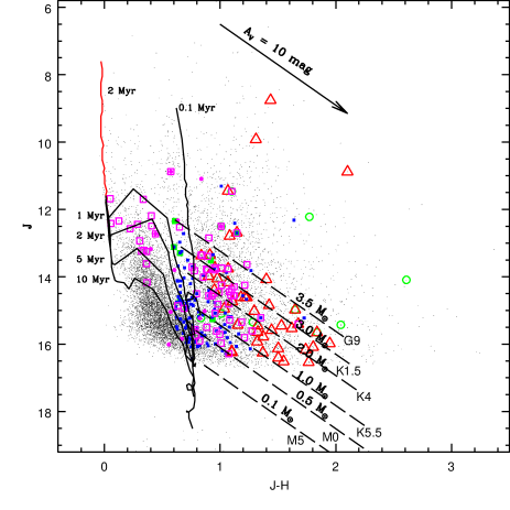
Figure 11: $J/(J-H)$ CMD for the stars in the CrW region. The isochrone of 2 Myr (Z = 0.02) by Marigo et al. (2008) and PMS isochrones of age 0.1, 1, 2, 5 and 10 Myr taken from Siess et al. (2000) corrected for a distance of 2.9 kpc and a reddening $E(B-V)_{min}$ = 0.25 are also shown. The symbols are the same as in Fig. 9 (see Sect. 4.3.1 for the classification scheme). The shown masses and spectral types have been taken from the 1 Myr PMS isochrone of Siess et al. (2000).

The CMDs are useful tools for studying the nature of the stellar population within star-forming regions. In Fig. 11, we plotted the $J/(J-H)$ CMD for all the YSOs identified in the previous sections having NIR counterparts and located in the CrW region. For cross-matching the $H\alpha$, X-ray, Spitzer, and Herschel identified YSOs with the 2MASS data, we took a search radius of 1 arcsec. For the FIR Herschel identified YSOs, we did not find any NIR counterpart. We used the relation $A_{J}/A_{V}$ = 0.265, $A_{H}/A_{V}$ = 0.155 (Cohen et al., 1981), isochrones for age- 2 Myr and PMS isochrones for ages 0.1, 1, 2, 5, and 10 Myr by Marigo et al. (2008) and Siess et al. (2000), respectively, to plot the CMD assuming a distance of 2.9 kpc and an extinction $E(B-V)_{min}$ = 0.25. In the present analysis, we used $R_{V}$ = 3.7 as discussed in Sect. 3.2. Different classes of probable YSOs are also shown in the figure. Most of the probable T Tauri, $H\alpha$ emission stars and IR excess stars have an apparent age under 1 Myr. The Spitzer identified YSOs are located mainly in two groups, one shows ages less than 1 Myr, whereas other groups have ages between 1$-$10 Myr. Smith et al. (2010) also find that the majority of YSOs in Carina have ages of $\sim$1 Myr.

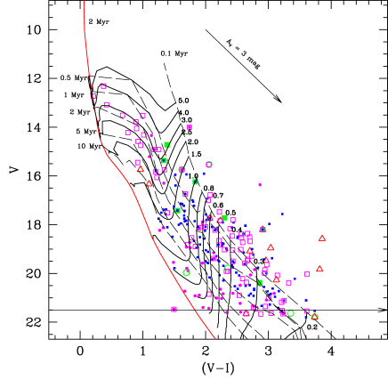
Figure 12: $V/(V-I)$ CMD for all the detected YSOs (symbols as in Fig. 9, see Sect. 4.2.2 for details). The isochrone for 2 Myr by Marigo et al. (2008) (continuous line) and PMS isochrones for 1, 2, 5, and 10 Myr by Siess et al. (2000) (dashed lines) are also shown. All the isochrones are corrected for a distance of 2.9 kpc and reddening $E(B-V)=0.25$. The horizontal line with arrow is the completeness limit of the observations.

The mass of the probable YSO candidates can be estimated by comparing their location on the CMD with the evolutionary models of PMS stars. The slanted dashed curve, taken from Siess et al. (2000), denotes the locus of 1 Myr old PMS stars having masses in the range of 0.1 to 3.5 $M_{\odot}$. To estimate the stellar masses, the $J$ luminosity is recommended rather than that of $H$ or $K$, because the $J$ band is less affected by the emission from circumstellar material (Bertout et al., 1988). The majority of the YSOs have masses in the range 3.5 to 0.5 $M_{\odot}$, indicating that these may be T Tauri stars. A few stars with a mass higher than 3.5 $M_{\odot}$ may be candidates for Herbig Ae/Be stars. Gaczkowski et al. (2013) state that this region exhibits a low number of very massive stars. However, since the more massive stars form more quickly and tend to be more obscured, and since they may not exhibit the same signatures of youth for as long a time as lower mass stars, a more extensive analysis is required to confirm their presence or absence in this region.

The NIR counterparts of YSOs in a nebular star-forming region are more easy to find than their optical counterparts. Therefore in the NIR CMD we have statistically more YSOs but to derive the exact age/mass of individual YSOs is somewhat difficult since at the lower end of the NIR CMD, the isochrones of different ages and masses nearly coincide with each other. Age and mass of individual YSOs can be derived more accurately using the optical CMDs.

Table 3: Sample of the optically identified YSOs along with their derived ages and masses. Error bars in magnitude and color represent formal internal (comparative) errors and do not include the color transformation and zero-point uncertainties.

ID	$\alpha$(J2000)	$\delta$(J2000)	$V\pm\sigma$	$(V-I)\pm\sigma$	Age $\pm\sigma$	Mass $\pm\sigma$	Technique
	($\degr$)	($\degr$)	(mag)	(mag)	(Mys)	(M⊙)	1,2,3,4,5,6
(1)	(2)	(3)	(4)	(5)	(6)	(7)	(8)
1	160.544858	-59.643538	12.316$\pm$0.009	0.373$\pm$0.018	0.9$\pm$0.2	3.7$\pm$0.2	1
2	160.586232	-59.898926	12.726$\pm$0.011	0.211$\pm$0.018	2.6$\pm$2.1	4.8$\pm$0.3	1
3	160.556561	-59.735036	13.079$\pm$0.011	0.422$\pm$0.014	1.4$\pm$0.2	2.8$\pm$0.3	1
4	159.827622	-59.759030	13.508$\pm$0.006	0.677$\pm$0.010	2.5$\pm$0.4	2.0$\pm$0.3	1
5	160.509158	-59.674841	13.527$\pm$0.009	1.000$\pm$0.014	1.4$\pm$0.2	3.4$\pm$0.3	1
–	–	–	–	–	–	–	–

¹ Spitzer identified sources, ² $H\alpha$ sources, ³ CTTS, ⁴ Chandra sources, ⁵ XMM-Newton sources, ⁶ Probable NIR excess
(This table is available in its entirety in a machine-readable form in the online journal. A portion is shown here for guidance regarding its form and content.)

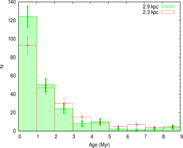
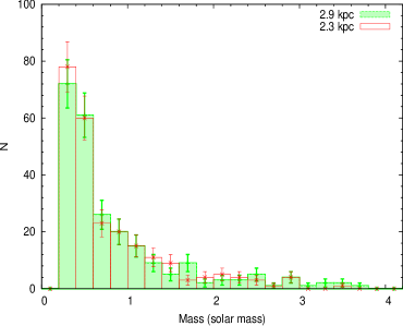
Figure 13: Histograms showing the distribution of YSOs ages (left panel) and masses (right panel) in the observed region. The green and red histograms are for the estimated ages and masses of YSOs assuming a distance of 2.9 kpc and 2.3 kpc, respectively. The error bars along ordinates represent $\pm\sqrt{N}$ Poisson errors.

4.3.2 Using optical CMD

In Fig. 12, the $V/(V-I)$ CMD has been plotted for the optical counterparts of YSOs identified in Sect. 4.2. We have taken the same 1 arcsec matching radius for identifying the optical counterparts of the presumed YSOs. Here also we have not found any optical counterpart of the Herschel identified YSOs. The dashed lines (for different ages 0.1, 0.5, 1, 2, 5 and 10 Myr) show PMS isochrones by Siess et al. (2000) and the post-main-sequence isochrone (continuous line) for 2 Myr by Marigo et al. (2008). These isochrones are corrected for the CrW distance (2.9 kpc) and minimum reddening ($E(B-V)=0.25$ mag, see previous section). It is clear from Fig. 12 that a majority of the sources have ages $<$ 1 Myr with a possible age spread up to 10 Myr.

The age and mass of the YSOs have been derived using the $V/(V-I)$ CMD. The Siess et al. (2000) isochrones have very coarse resolution (30 points for their whole mass range of 0.1 to 7 M_⊙); therefore, for a better estimation of mass, these isochrones were interpolated (2000 points). We used photometric errors along with the error in the distance modulus and reddening to draw an error box around each data point. In this box, we generated 500 random points using Monte Carlo simulations. For each generated point, we calculated the age and mass as derived from the nearest passing isochrone. For this study we used a bin size of 0.1 Myr for the Siess et al. (2000) isochrones. At the end we took the mean and standard deviation as the final derived values.

It is important to note that estimating the ages and masses of the PMS stars by comparing their locations in the CMDs with theoretical isochrones is prone to both random and systematic errors (see Hillenbrand, 2005; Hillenbrand et al., 2008; Chauhan et al., 2009, 2011). The effect of random errors due to photometric errors and reddening estimation in determining the ages and masses has been evaluated by propagating the random errors to their observed measurements by assuming a normal error distribution and using Monte Carlo simulations (cf. Chauhan et al., 2009). The systematic errors could be due to the use of different PMS evolutionary models and an error in the distance estimation. Barentsen et al. (2011) mention that the ages may be incorrect by a factor of two owing to systematic errors in the model. The presence of variable extinction in the region will not affect the age estimation significantly because the reddening vector in the $V/(V-I)$ CMD is nearly parallel to the PMS isochrone.

The presence of binaries may also introduce errors into the age determination. Binarity will brighten the star, consequently the CMD will yield a lower age estimate. In the case of an equal-mass binary, we expect an error of $\sim$50% to $\sim$60% in the PMS age estimation. However, it is difficult to estimate the influence of binaries/variables on the mean age estimation because the fraction of binaries/variables is not known. In the study of TTSs in the Hii region IC 1396, Barentsen et al. (2011) point out that the number of binaries in their sample of TTSs could be very low since close binaries lose their disk significantly faster than single stars (cf. Bouwman et al., 2006).

We have calculated ages and masses for 241 optically identified individual YSOs classified using different schemes (see Table 3). Here we would like to point out that out of six optically identified probable NIR excess stars, five have ages $\lesssim$1 Myr. They may be YSOs that are deeply embedded and are formed by the collapse of the core of a molecular cloud. Estimated ages and masses of the YSOs range from $\sim$0.1 to 10 Myr and $\sim$0.3 to 4.8 M_⊙, respectively. This age range indicates a wide spread in the formation of stars in the region. The histograms of age and mass distribution of YSOs are shown in Fig. 13.

As stated in Sect. 3.3, several authors have used different distances (2.3 kpc) than ours (2.9 kpc) for the Carina nebula. Therefore, we also examined the above results (ages and masses of YSOs) for the distance of 2.3 kpc. The ages and masses of YSOs are once again derived using the same procedure as described above and the corresponding histograms are overplotted in Fig. 13. As can be seen in this figure, both derived values are more or less similar within their corresponding errors, although there are slight differences in the number of YSOs that are less than 1 Myr. By looking at this figure, we can safely conclude that the majority of the YSOs are younger than 1 Myr and have a mass lower than 2 M_⊙. These age and mass are comparable with the lifetime and mass of TTSs.

4.4 Initial mass function

The distribution of stellar masses that formed in one star-formation event in a given volume of space is called the initial mass function (IMF), and together with the star formation rate, the IMF dictates the evolution and fate of galaxies and star clusters. The effects of environment may be more revealing at the low-mass end of the IMF, since one might imagine that the lower end of the mass spectrum is most strongly affected by external effects. The goals of this study are to identify the PMS populations in order to study the IMF down to the substellar regime.

The mass function (MF) is often expressed by a power law, $N(\log m)\propto m^{\Gamma}$ and the slope of the MF is given as

$$\Gamma=d\log N(\log m)/d\log m$$

where $N(\log m)$ represents the number of stars per unit logarithmic mass interval.

The IMF in the Galaxy has been estimated empirically. The first such determination by Salpeter (1955) gave $\Gamma=-1.35$ for the stars in the mass range $0.4\leq$ M/M${}_{\odot}\leq 10$. However, more recent works (e.g., Miller & Scalo, 1979; Scalo, 1986; Rana, 1991; Kroupa, 2002) suggest that the mass distribution deviates from a pure power law. It has been shown (see, e.g., Corbelli et al., 2005; Scalo, 1986, 1998; Kroupa, 2002; Chabrier, 2003) that, for masses above $\sim$1M_⊙, the IMF can generally be approximated by a declining power law with a slope similar to what is found by Salpeter (1955). However, it is now clear that this power law does not extend to masses much below $\sim$1M_⊙. The distribution becomes flatter below 1 M_⊙ and turns off at the lowest stellar masses. It has also often been claimed that some (very) massive star-forming regions have a truncated IMF, i.e., contain much smaller numbers of low-mass stars than expected from the field IMF. However, most of the more recent and sensitive studies of massive star-forming regions (see, e.g., Liu et al., 2009; Espinoza et al., 2009) find the numbers of low-mass stars in agreement with the expectation from the “normal” field star IMF. Preibisch et al. (2011c) confirm these results for the Carina Nebula and support the assumption of a universal IMF (at least in our Galaxy). In consequence, this result also supports the notion that OB associations and very massive star clusters are the dominant formation sites of the galactic field star population, as already suggested by Miller & Scalo (1978).

We have optically identified 241 YSOs (cf. Sect. 4.2) in the region of CrW and then calculated their masses (cf. Sect. 4.3) with the help of optical CMD using the theoretical PMS of Siess et al. (2000). Here we would like to mention that for our photometry, the completeness limit is 0.5 M_⊙ for a distance of 2.9 kpc. The MF of the CrW region is plotted in Fig. 14. The slope of the MF ‘$\Gamma$’ in the mass range 0.5 $<$ M/M_⊙ $<$ 4.8 comes out to be $-1.13\pm 0.20$, which is a bit shallower than the value given by Salpeter (1955), and there seems to be no break in the slope at M $\sim$1 M_⊙, as has been noticed in previous works (Sharma et al., 2007; Pandey et al., 2008; Jose et al., 2008). On the other hand, Preibisch et al. (2011c) show that, down to a mass limit around 0.5 $-$ 1 M_⊙, the shape of the IMF in Carina is consistent with that in Orion (and thus the field IMF). Their results directly show that there is clearly no deficit of low-mass stars in the CNC down to $\sim$1M_⊙.

Figure 14: Plot of the mass function in the CrW region. Log $\Phi$ represents log$N$(log $m$). The error bars represent $\pm\sqrt{N}$ errors. The solid line shows a least-squares fit over the entire mass range 0.5 $<$ M/M${}_{\odot}<$ 4.8. Open and filled circles represent the points below and above the completeness limit of our data, respectively.

4.5 $K$-band luminosity function

The $K$-band luminosity function (KLF) is the number of stars as a function of $K$-band magnitude. It is frequently used in studies of young clusters and star-forming regions as a diagnostic tool of the mass function and the star formation history of their stellar populations. The interpretation of KLF has been presented by several authors (see, e.g., Zinnecker et al., 1993; Muench et al., 2000; Lada & Lada, 2003, and references therein).

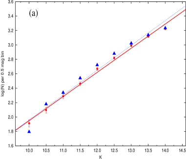
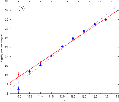
Figure 15: (a) Comparison between the observed KLF in the reference field (red filled circles) and the simulated KLF from star counts modeling (blue filled triangles). If the star counts represent the number N of stars in a bin, the associated error bars are $\pm\sqrt{N}$. The KLF slope ($\alpha$, see Sect. 4.5) of the reference field (solid line) is $0.34\pm 0.01$. The simulated model (dashed line) also gives the same value of slope ($0.34\pm 0.02$). (b) The KLF for the CrW region (filled red circles) and the simulated star counts (blue filled triangles). In the magnitude range 10.5 $-$ 14.25, the best-fit KLF slope ($\alpha$) for the CrW region (solid line) is $0.31\pm 0.01$, whereas for the model (dashed line), after taking extinction into account, it comes out to be $0.36\pm 0.02$.

To obtain the KLF, it is essential to take the incompleteness of the data and the foreground and background source contaminations into account. The completeness of the data is estimated using the ADDSTAR routine of DAOPHOT as described in Section 2.2. To consider the foreground/background field star contaminations, we used both the Besançon Galactic model of stellar population synthesis (Robin et al., 2003) and the nearby reference field stars. Star counts are predicted using the Besançon model in the direction of the control field. We checked the validity of the simulated model by comparing the model KLF with that of the control field and found that both KLFs match rather well. An advantage to using the model is that we can separate the foreground (d $<$ 2.9 kpc) and background (d $>$ 2.9 kpc) field stars. As mentioned in Section 3.1, the foreground extinction using optical data was found to be $A_{V}\sim$0.93 mag. The model simulations with $A_{V}$ = 0.93 mag and d $<$ 2.9 kpc gives the foreground contamination.

The background population (d $>$ 2.9 kpc) was simulated with $A_{V}$ = 3.4 mag in the model. We thus determined the fraction of the contaminating stars (foreground + background) over the total model counts. This fraction was used to scale the nearby reference field. The KLF is expressed by the power law

${{\it{d}N(K)}\over{\it{d}K}}\propto 10^{\alpha K}$ ,

where ${\it{d}N(K)}\over{\it{d}K}$ is the number of stars per 0.5 magnitude bin, and $\alpha$ is the slope of the power law.

Figures 15a and b show the KLF for the reference field and CrW region, respectively. The $\alpha$ for the reference field and simulated model is $0.34\pm 0.01$ and $0.34\pm 0.02$, respectively. Similarly $\alpha$ for the CrW region is $0.31\pm 0.01$, whereas for the model, after taking the extinction into account, it comes out to be $0.36\pm 0.02$.

5 Discussion: star formation scenario in the CrW region

Povich et al. (2011) using Spitzer MIR data identified 1439 YSOs (Pan Carina YSO Catalog) in the field surveyed by the CCCP. The spatial distribution of these YSOs throughout the Carina Nebula shows a highly complex structure with clustering at several positions. The majority of YSOs identified by them are located inside the Hii cavities near, but less frequently within, the boundaries of dense molecular clouds and the ends of the pillars. They also found that the high concentration of the intermediate mass YSOs is in Tr 14 itself. They have concluded that the recent star formation history in the Carina Nebula has been driven or at least regulated by feedback from the massive stars.

Recently, Gaczkowski et al. (2013) identified 642 YSOs in the Carina Complex with the help of FIR Herschel data. These YSOs are also found to be highly heterogeneously distributed in the region, and they do not follow the distribution of cloud mass. Gaczkowski et al. (2013) show that the Herschel selected YSO candidates are located near the irradiated surfaces of clouds (see Fig. 16) and pillars, whereas the Spitzer selected ‘YSO’ candidates (Povich et al., 2011) often surround these pillars. This characteristic spatial distribution of the young stellar populations in different evolutionary stages has been related by Gaczkowski et al. (2013) to the idea that the advancing ionization fronts compress the clouds and lead to cloud collapse and star formation in these clouds, just ahead of the ionization fronts. They further state that some fraction of the cloud mass is transformed into stars (and these are the YSOs detected by Herschel), while another fraction of the cloud material is dispersed by the process of photo-evaporation. As time proceeds, the pillars shrink, and a population of slightly older YSOs is left behind and revealed after the passage of the ionization front. Their results provide additional evidence that the formation of these YSOs was indeed triggered by the advancing ionization fronts of the massive stars as suggested by the theoretical models (see Gritschneder et al., 2010).

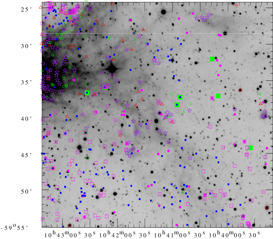
Figure 16: Spatial distributions of different classes of YSOs. Various symbols are overlaid on the WISE 4.6 $\mu$m image. The filled square symbols represent X-ray identified sources (XMM-Newton bigger green, Chandra sources small blue). Open magenta squares, open red triangles, filled magenta circles, and open green circles are Spitzer-identified YSOs, CTTSs, $H\alpha$ emission stars, and probable NIR-excess YSOs, respectively. Purple star symbols are Herschel YSO sources. The abscissae and the ordinates represent RA and Dec, respectively for the J2000 epoch.

Roccatagliata et al. (2013) with the help of the wide-field Herschel SPIRE and PACS maps, determined the temperatures, surface densities, and the local strength of the far-UV irradiation for all the cloud structures over the entire spatial extent of the CNC. They find that the density and temperature structure of the clouds in most parts of the CNC are dominated by the strong feedback from the numerous massive stars, rather than by random turbulence. They also conclude that the CNC is forming stars in a particularly efficient way, which is a consequence of triggered star formation by radiative cloud compression due to numerous high mass stars.

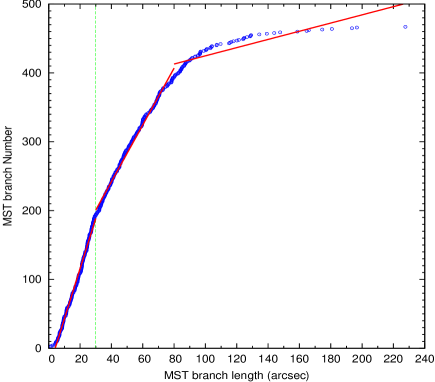
(a) a

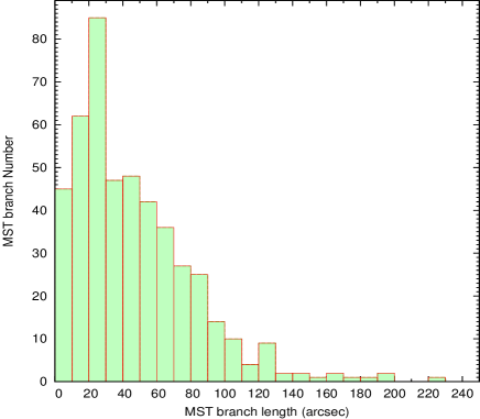
(b) b

Figure 17: Cumulative distribution of the MST branch lengths. In panel (a), the solid lines represent the linear fits to the points smaller and larger than the chosen critical branch length. The critical radius is shown by a vertical line. Panel (b) is the histogram of the MST branch lengths for the YSOs in the CrW region (see text).

In the center of Carina, there are the young clusters, Trumpler 14, 15, and 16, that host about 80% of the high mass stars of the entire complex (Roccatagliata et al., 2013). This is also the hottest region of the nebula with temperatures ranging between 30 and 50 K, whereas the molecular cloud at the western side of Tr 14 has a temperature of about 30 K and a decrease in density from the inner to the edge part (Roccatagliata et al., 2013). Our studied region CrW contains this cloud, which can be seen in our infrared extinction map (see Fig. 7). In Fig. 16, different classes of YSOs identified in our study are overlaid on the WISE 4.6 $\mu$m (MIR) image. We can easily see the extension of the dust lane in the figure from northeast to southwest of the CrW region. The northeast region contains the outer most part of the cluster Tr 14 along with the high density region of the molecular cloud (see Fig. 7). Smith & Brooks (2008) show the spatial relationship of Tr 14, the ionized gas, the PDR emission, the molecular gas, and the dust lane. The brightest molecular emission is concentrated towards the dark western dust lane offset from the center of Tr 14 by 4 arcmin. The radio continuum for emission source “Car I” can also be seen here at the interface of the dust lane and the bright Hii region. Between this source and the molecular cloud, a widespread PDR emission can also be seen in the form of an arc like PAH emission feature at 3.3 $\mu$m (Rathborne et al., 2002). At a projected distance of $\sim$2 pc, the UV output of Tr 14 dominates the other Carina Nebula clusters such as Tr 16 in determining the local flux at the PDR in the northern cloud (Brooks et al., 2003; Smith, 2006a; Smith & Brooks, 2008). This spatial sequence of Tr 14, radio source, PAH emission, and then strong molecular emission delineates a classical edge-on PDR (Brooks et al., 2003). The edge of this region contains many Spitzer-identified YSOs. The alignment of the YSOs in this region may be due to the star formation triggered by high mass stars of Tr 14.

The Herschel-identified YSOs (Gaczkowski et al., 2013) are located mainly in the high density region of the molecular clumps and in small groupings at several places along the dust lane. Gaczkowski et al. (2013) have derived an age of $\sim$0.1 Myr for their sample of YSOs. The probable NIR excess stars identified in this study also follow this region. For some of them, we derived ages $\lesssim$1 Myr. These sets of identified YSOs are basically very young in nature and are embedded in the cores of the molecular cloud. We could not say anything about the northwest region of CrW, which is not well covered by previous surveys.

Smith et al. (2010) observed in their western mosaic (which contains most of our observed region including the dark lane, see their Fig. 3), the YSOs density of around 500 sources/deg² with little signs of clustering. In this study we have identified 467 YSOs falling in the CrW region. The overall density of this region then turns out to be $\sim$1700 sources/deg² which is higher than three times the YSOs density given by Smith et al. (2010). Here it is worthwhile to mention that the PCYC used in previous studies has a sensitivity problem at the ionization front between Tr 14 and the Car I molecular cloud core to the west (Yonekura et al., 2005; Ascenso et al., 2007) where the diffuse MIR nebular emission is bright (Povich et al., 2011).

Table 4: The YSO cores identified in the CrW region and their characteristics.

Core	Radius	Number of YSOs	Number	Median
number	(pc)	in core (N)	density (N/pc2)	branch length (pc)
A	0.45	6	9.43	0.32
B	0.37	6	13.95	0.26
C	0.51	8	9.79	0.36
D	0.56	7	7.11	0.33
E	0.18	4	39.30	0.12
F	0.26	5	23.54	0.20
G	0.39	4	8.37	0.36
H	0.49	6	7.95	0.31
I	0.64	6	4.66	0.30
J	0.44	7	11.51	0.28
Average	0.43	5.9	13.56	0.28

The complex observational patterns (e.g., filaments, bubbles, and irregular clumps, etc.) in a molecular cloud such as Carina nebula are resulting from the interplay of fragmentation processes. The star formation usually takes place inside the dense cores of the molecular clouds, and the YSOs often follow clumpy structures of their parent molecular clouds (see, e.g., Gomez et al., 1993; Lada et al., 1996; Motte et al., 1998; Allen et al., 2002; Gutermuth et al., 2005; Teixeira et al., 2006; Winston et al., 2007; Gutermuth et al., 2008). Recently, fragmentations in gas with turbulence (e.g., Ballesteros-Paredes et al., 2007) and magnetic fields (e.g., Ward-Thompson et al., 2007) have been discussed, leading to detailed predictions of the distributions of fragment spacings. The spatial distribution of YSOs in a region can be analyzed in terms of a typical spacing between them in order to compare this spacing to the Jeans fragmentation scale for a self-gravitating medium with thermal pressure (Gomez et al., 1993). Some recent observations of star-forming regions have been analyzed in terms of the distribution of nearest neighbor (NN) distances (see Gutermuth et al., 2005; Teixeira et al., 2006) and find a strong peak in their histogram of NN spacings for the protostars in young embedded clusters. This peak indicated a significant degree of Jeans fragmentation, since this most frequent spacing agreed with an estimate of the Jeans length for the dense gas within which the YSOs are embedded. These results also suggest that the tendency for a narrow range of spacings among YSOs in a cluster can last into the Class II phase of YSO evolution.

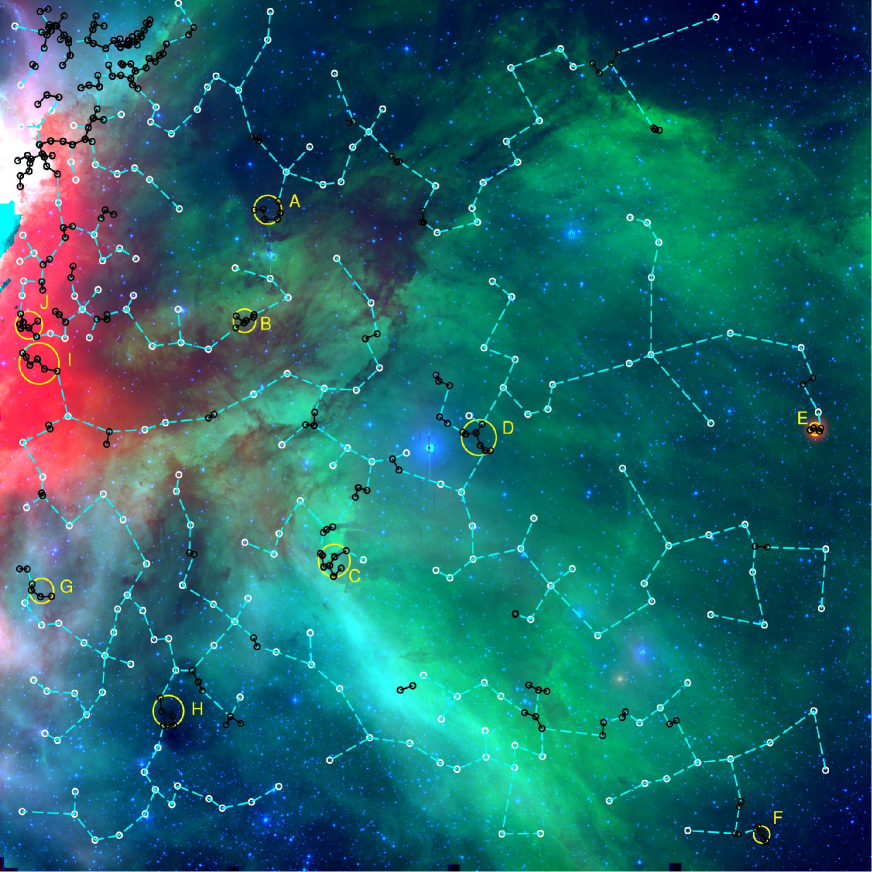
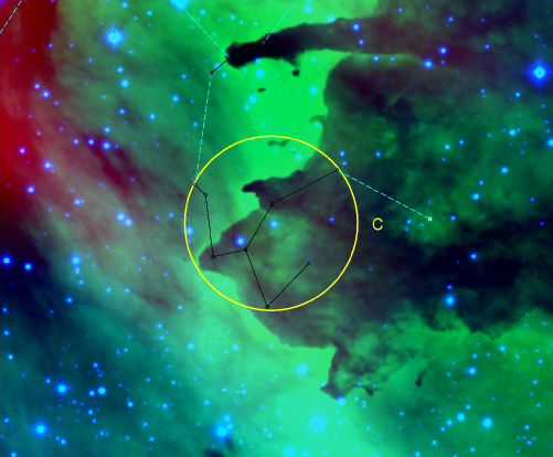
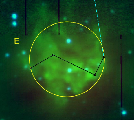
Figure 18: Top: Minimal spanning tree of the YSOs overplotted on a color composite image of the CrW region (WISE 22 $\mu$m (red), $H\alpha$ band (green), and $V$ band (blue) images). WR 22 is situated in the center. The white circles connected with dotted lines, and black circles connected with solid lines are the branches that are larger and smaller than the basic critical length, respectively. The identified ten cluster cores are encircled with yellow color and labeled with A to J. Bottom: Two zoomed images of YSO cores, C and E, are shown in the lower left and right panels, respectively (see text for detail).

Recently, Gutermuth et al. (2009) have done a complete characterization of the spectrum of source spacings using the minimal spanning tree (MST) of source positions. The MST is defined as the network of lines, or branches, that connect a set of points together such that the total length of the branches is minimized and there are no closed loops (see, e.g., Cartwright & Whitworth, 2004; Gutermuth et al., 2009, and references therein). Gutermuth et al. (2009) demonstrate that the MST method yields a more complete characterization than NN method. Therefore, for the present study, we used the same MST algorithm to analyze the spatial distribution of YSOs in the CrW region.

In Fig. 17b, we plotted the histogram of MST branch lengths for the YSOs in the CrW region. From this plot, it is clear that they have a peak at small spacings and that they also have a relatively long tail of large spacings. Peaked distance distributions typically suggest a significant subregion (or subregions) of relatively uniform, elevated surface density. By adopting an MST length threshold, we can isolate those sources that are closer together than this threshold, yielding populations of sources that make up a local surface density enhancement. To get this threshold distance, in Fig. 17a, we plotted the cumulative distribution function (CDF) for the branch length of YSOs. The curve shows three different slopes: first a steep-sloped segment at short spacings then a transition segment that approximates the curved character of the intermediate-length spacings, and finally a shallow-sloped segment at long spacings. For the present study, we have chosen the peak in the histogram ($\sim$30 arcsec $\sim$0.42 pc), which corresponds to the first steep-sloped segment, as a threshold or critical length.

In Fig  18, the results from MST analysis are overplotted on the RGB image of the CrW region. This image was created using red, green, and blue colors for the WISE 22 $\mu$m, $H\alpha$, and $V$ band images, respectively. Circles and MST connections in black deal with the objects that are more closely spaced than the critical length (0.42 pc).

A close inspection of Fig. 18 reveals that the CrW region exhibits heterogeneous structures, and there are several close concentrations of YSOs distributed along the molecular clumps. Prominent YSO clustering can be seen in the northeastern part of this figure and are possibly part of the star cluster Tr 14. There are also ten cores (having MST branch lengths less than the critical distance) distributed along the molecular cloud (indicated in Fig.18). A close view of the cores C and E can be seen in the lower left and right panels in Fig 18. The details about these cores have been given in Table 4. The majority of the members of all these cores are the YSOs identified in the Herschel survey having very young ages. Our result agrees with the conclusions of Gutermuth et al. (2009) and Günther et al. (2012), indicating that the young protostars are found in a region having marginally higher surface densities than the more evolved PMS stars. The average of median branch length and core radius is found to be 0.28 pc and 0.43 pc, respectively (see Table 4).

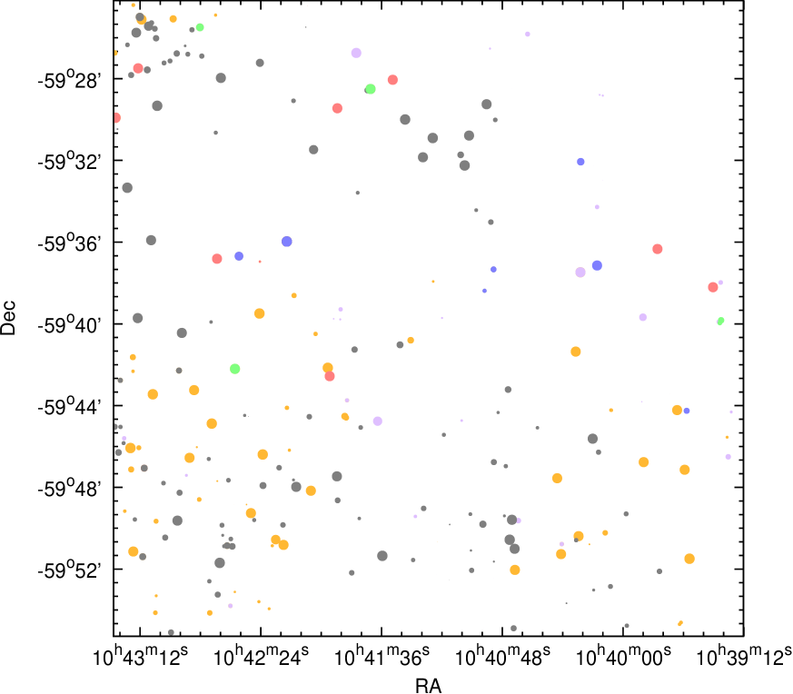
Figure 19: Spatial distribution of the optically identified YSOs in the CrW region. The size of the symbols represents the age of the YSO, i.e. bigger the size younger the YSO is. Various colors represent YSOs identified using different schemes (Spitzer - orange, $H\alpha$ - purple, CTTS - red, Chandra sources - black, XMM-Newton - blue, and IR excess - green).

To check the role of WR 22 in the formation of stars in this region, we tried to look at the spatial distribution of YSOs (Fig. 19) with optical counterparts (whose age has been derived using the $V/(V-I)$ CMD, cf. Sect. 4.3.2) in the CrW region. The general observation is that within the detection limit of optical observations, the YSOs show mixed populations of different ages throughout the CrW region. The extreme northeastern region contains a group of YSOs that are under the direct influence of the high-mass stars of Tr 14, and it also shows a mixed population. For most of the YSOs in the dust lane, we have not found their optical counterparts. This age distribution around CrW does not show any trend even in the presence of a very massive star such as WR 22. It seems that WR 22 has not influenced these YSOs much. Smith et al. (2010) presented Spitzer observations of a part of the CrW region studied here. These authors reached similar conclusions, suggesting that this very massive star may be projected in the foreground or background compared to the surrounding molecular gas, or it could have only recently arrived at its present location.

6 Summary and conclusions

Although the center of the Carina nebula has been studied extensively, the outer region has been neglected due to the absence of wide field optical surveys. In this study, we investigated a wide field ($32^{\prime}\times 31^{\prime}$) located in the west of the Carina nebula and centered on the massive binary WR 22. To our knowledge, this is the first detailed study of this region. We used deep optical ($UBVRI$) and $H\alpha$ photometric data obtained with the WFI instrument at the ESO/MPG 2.2 m telescope (La Silla). Our $V$ band photometry is complete up to $\sim$21.5 mag. Low-resolution spectroscopy along with Chandra, XMM-Newton, and 2MASS archival data sets, was also used in this analysis. We generated various combinations of optical and NIR TCD, CMDs and calculated several parameters such as reddening, reddening law, etc. We also identified the YSOs located in the region and studied their spatial distribution using the MST method. Ages and masses of the 241 YSOs having optical counterparts, were derived based on $V/(V-I)$ CMD. These YSOs have been further used to constrain the IMF of the region. The main scientific results from our study are as follows

• The region shows a large amount of differential reddening with minimum and maximum $E(B-V)$ values of 0.25 and 1.1 mag., respectively. This region shows an unusual reddening law with a total-to-selective extinction ratio $R_{V}=3.7\pm 0.1$.

• The MK spectral types for a subsample of 15 X-ray emitting sources in the CrW region are established that indicates that the majority of them are late spectral type stars. There are three sources belonging to each O, A, and F spectral types; however, six sources are of spectral type G.

• We cross-correlated the 43 XMM-Newton X-ray sources from Claeskens et al. (2011) with our optical photometry and found that 34 of them are well matched. Out of these 34 sources, 7 have been identified as YSOs. We also cross-identified the Chandra X-ray sources (1465 in our region) with our source list and found 469 objects with optical/NIR counterparts. In total, 119 X-ray sources are identified as YSOs, four of them in common with XMM-Newton.

• We collected a sample of 467 YSOs identified in the CrW region based on their IR-excess, $H\alpha$ and X-ray emission. In some cases, the same YSOs were identified in more than one scheme. Out of these, there are 41 $H\alpha$ emitters, 105 Herschel identified YSOs, 136 Spitzer identified YSOs, and 225 2MASS identified YSOs in our list. The YSO density for the CrW region turns out to be $\sim$1700 sources/degree², which is higher when compared to the reported values (500 sources/degree², Smith et al. 2010).

• We calculated the age and mass of 241 individual optically identified YSOs. Estimated ages and masses of the YSOs range from $\sim$0.1 to 10 Myr and $\sim$0.3 to 4.8 M_⊙, respectively. This age range indicates a wide spread in the formation of stars in the region. The majority of these YSOs are younger than 1 Myr, and their mass is below 2 M_⊙.

• We derived the IMF and calculated the slope ‘$\Gamma$’ in the CrW region. In the mass range $0.5<$ M/M${}_{\odot}<4.8$, it comes out as $-1.13\pm 0.20$ which is a bit shallower than the value of $-1.35$ given by Salpeter (1955), and there seems to be no break in the slope at M $\sim$1M_⊙. The slope of the K-band luminosity function is found to be $\alpha=0.31\pm 0.01$.

• The spatial distribution of all 467 YSOs has been studied in detail. The edge of the irradiated surface between Tr 14 and the molecular cloud contains many Spitzer identified YSOs whose formation was probably triggered by the high-mass stars of Tr 14. The high-density region of molecular clumps contains many probable NIR excess stars, as well as Herschel-identified YSOs that are very young in age ($\lesssim$1 Myr).

• We used the well-established MST method to identify local density enhancements in the YSO distributions. The northeastern part of the studied region presents a more prominent YSO clustering. However, there are at least ten cores of four or more very young YSO members distributed all over the CrW region and having different core radii. The average core radii and median branch length values for these cores are found to be 0.43 pc and 0.28 pc, respectively. The YSOs having optical counterparts in CrW are uniformly distributed having mixed population of different ages. The age distribution around CrW does not show any trend in the presence of the very massive star WR 22. It seems that WR 22 is a foreground/background star which has not influenced the formation of YSOs in the CrW region.

References

- Abbott & Conti (1987) Abbott, D. C. & Conti, P. S. 1987, ARA&A, 25, 113
- Allen et al. (2002) Allen, L. E., Myers, P. C., Di Francesco, J., et al. 2002, ApJ, 566, 993
- Arnett (1995) Arnett, D. 1995, ARA&A, 33, 115
- Arnett (1996) Arnett, D. 1996, Supernovae and nucleosynthesis. an investigation of the history of matter, from the Big Bang to the present, Princeton University Press.
- Ascenso et al. (2007) Ascenso, J., Alves, J., Vicente, S., & Lago, M. T. V. T. 2007, A&A, 476, 199
- Ballesteros-Paredes et al. (2007) Ballesteros-Paredes, J., Klessen, R. S., Mac Low, M.-M., & Vazquez-Semadeni, E. 2007, Protostars and Planets V, eds. B. Reipurth, D. Jewitt, & K. Keil, University of Arizona Press, Tucson, 63
- Barentsen et al. (2011) Barentsen, G., Vink, J. S., Drew, J. E., et al. 2011, MNRAS, 415, 103
- Becker & Fenkart (1971) Becker, W. & Fenkart, R. 1971, A&AS, 4, 241
- Bertout (1989) Bertout, C. 1989, ARA&A, 27, 351
- Bertout et al. (1988) Bertout, C., Basri, G., & Bouvier, J. 1988, ApJ, 330, 350
- Bessell & Brett (1988) Bessell, M. S. & Brett, J. M. 1988, PASP, 100, 1134
- Bouwman et al. (2006) Bouwman, J., Lawson, W. A., Dominik, C., et al. 2006, ApJ, 653, L57
- Briceño et al. (2007) Briceño, C., Preibisch, T., Sherry, W. H., et al. 2007, Protostars and Planets V, eds. B. Reipurth, D. Jewitt, & K. Keil, University of Arizona Press, Tucson, 345
- Brooks et al. (2003) Brooks, K. J., Cox, P., Schneider, N., et al. 2003, A&A, 412, 751
- Brooks et al. (2001) Brooks, K. J., Storey, J. W. V., & Whiteoak, J. B. 2001, MNRAS, 327, 46
- Broos et al. (2010) Broos, P. S., Townsley, L. K., Feigelson, E. D., et al. 2010, ApJ, 714, 1582
- Carraro & Patat (2001) Carraro, G. & Patat, F. 2001, A&A, 379, 136
- Carraro et al. (2001) Carraro, G., Patat, F., & Baumgardt, H. 2001, A&A, 371, 107
- Carraro et al. (2004) Carraro, G., Romaniello, M., Ventura, P., & Patat, F. 2004, A&A, 418, 525
- Cartwright & Whitworth (2004) Cartwright, A. & Whitworth, A. P. 2004, MNRAS, 348, 589
- Chabrier (2003) Chabrier, G. 2003, PASP, 115, 763
- Chauhan et al. (2011) Chauhan, N., Pandey, A. K., Ogura, K., et al. 2011, MNRAS, 415, 1202
- Chauhan et al. (2009) Chauhan, N., Pandey, A. K., Ogura, K., et al. 2009, MNRAS, 396, 964
- Chini & Kruegel (1983) Chini, R. & Kruegel, E. 1983, A&A, 117, 289
- Chini & Wargau (1990) Chini, R. & Wargau, W. F. 1990, A&A, 227, 213
- Claeskens et al. (2011) Claeskens, J.-F., Gosset, E., Nazé, Y., Rauw, G., & Vreux, J.-M. 2011, A&A, 525, A142
- Clariá (1977) Clariá, J. J. 1977, A&AS, 27, 145
- Cohen et al. (1981) Cohen, J. G., Persson, S. E., Elias, J. H., & Frogel, J. A. 1981, ApJ, 249, 481
- Conti et al. (1979) Conti, P. S., Niemela, V. S., & Walborn, N. R. 1979, ApJ, 228, 206
- Corbelli et al. (2005) Corbelli, E., Palla, F., & Zinnecker, H. 2005, in The Initial Mass Function 50 Years Later, Vol. 327, Astrophysics and Space Science Library
- Cox (1995) Cox, P. 1995, in The Eta Carinae Region: A Laboratory of Stellar Evolution, eds. V. Niemela, N. Morrell, & A. Feinstein, Rev. Mexicana Astron. Astrofis. Ser. Conf., 2, 105
- Crowther (2007) Crowther, P. A. 2007, ARA&A, 45, 177
- Crowther et al. (1995) Crowther, P. A., Hillier, D. J., & Smith, L. J. 1995, A&A, 293, 403
- Cutri et al. (2003) Cutri, R. M., Skrutskie, M. F., van Dyk, S., et al. 2003, VizieR Online Data Catalog, 2246, 0
- de Graauw et al. (1981) de Graauw, T., Lidholm, S., Fitton, B., et al. 1981, A&A, 102, 257
- DeGioia-Eastwood et al. (2001) DeGioia-Eastwood, K., Throop, H., Walker, G., & Cudworth, K. M. 2001, ApJ, 549, 578
- Dickel (1974) Dickel, H. R. 1974, A&A, 31, 11
- Dufour et al. (1998) Dufour, R. J., van Orsow, D., Walter, D. K., Hester, J. J., & Currie, D. G. 1998, in Astrophysical plasmas - near and far, eds. R. J. Dufour, & S. Torres-Peimbert, Rev. Mexicana Astron. Astrofis. Ser. Conf., 7, 217
- Elmegreen (1998) Elmegreen, B. G. 1998, in Origins, eds. C. E. Woodward, J. M. Shull, & H. A. Thronson, Jr., ASP Conf. Ser., 148, 150
- Espinoza et al. (2009) Espinoza, P., Selman, F. J., & Melnick, J. 2009, A&A, 501, 563
- Feigelson et al. (2002) Feigelson, E. D., Broos, P., Gaffney, III, J. A., et al. 2002, ApJ, 574, 258
- Feigelson & Montmerle (1999) Feigelson, E. D. & Montmerle, T. 1999, ARA&A, 37, 363
- Feinstein (1981) Feinstein, A. 1981, PASP, 93, 202
- Feinstein (1983) Feinstein, A. 1983, Ap&SS, 96, 293
- Feinstein (1995) Feinstein, A. 1995, in The Eta Carinae Region: A Laboratory of Stellar Evolution, eds. V. Niemela, N. Morrell, & A. Feinstein, Rev. Mexicana Astron. Astrofis. Ser. Conf., 2, 57
- Feinstein et al. (1973) Feinstein, A., Marraco, H. G., & Muzzio, J. C. 1973, A&AS, 12, 331
- Fitzgerald & Mehta (1987) Fitzgerald, M. P. & Mehta, S. 1987, MNRAS, 228, 545
- Forte (1978) Forte, J. C. 1978, AJ, 83, 1199
- Gaczkowski et al. (2013) Gaczkowski, B., Preibisch, T., Ratzka, T., et al. 2013, A&A, 549, A67
- Garay & Lizano (1999) Garay, G. & Lizano, S. 1999, PASP, 111, 1049
- Garmire et al. (2003) Garmire, G. P., Bautz, M. W., Ford, P. G., Nousek, J. A., & Ricker, Jr., G. R. 2003, in Society of Photo-Optical Instrumentation Engineers (SPIE) Conf. Ser., eds. J. E. Truemper & H. D. Tananbaum, Vol. 4851, 28–44
- Getman et al. (2005) Getman, K. V., Flaccomio, E., Broos, P. S., et al. 2005, ApJS, 160, 319
- Ghosh et al. (1988) Ghosh, S. K., Iyengar, K. V. K., Rengarajan, T. N., et al. 1988, ApJ, 330, 928
- Gomez et al. (1993) Gomez, M., Hartmann, L., Kenyon, S. J., & Hewett, R. 1993, AJ, 105, 1927
- Gosset et al. (2009) Gosset, E., Nazé, Y., Sana, H., Rauw, G., & Vreux, J.-M. 2009, A&A, 508, 805
- Gosset et al. (1991) Gosset, E., Remy, M., Manfroid, J., et al. 1991, Information Bulletin on Variable Stars, 3571, 1
- Grabelsky et al. (1988) Grabelsky, D. A., Cohen, R. S., Bronfman, L., & Thaddeus, P. 1988, ApJ, 331, 181
- Gritschneder et al. (2010) Gritschneder, M., Burkert, A., Naab, T., & Walch, S. 2010, ApJ, 723, 971
- Guetter & Vrba (1989) Guetter, H. H. & Vrba, F. J. 1989, AJ, 98, 611
- Günther et al. (2012) Günther, H. M., Wolk, S. J., Spitzbart, B., et al. 2012, AJ, 144, 101
- Gutermuth et al. (2009) Gutermuth, R. A., Megeath, S. T., Myers, P. C., et al. 2009, ApJS, 184, 18
- Gutermuth et al. (2005) Gutermuth, R. A., Megeath, S. T., Pipher, J. L., et al. 2005, ApJ, 632, 397
- Gutermuth et al. (2008) Gutermuth, R. A., Myers, P. C., Megeath, S. T., et al. 2008, ApJ, 674, 336
- Hamaguchi et al. (2007) Hamaguchi, K., Petre, R., Matsumoto, H., et al. 2007, PASJ, 59, 151
- Hamann et al. (1991) Hamann, W.-R., Duennebeil, G., Koesterke, L., Wessolowski, U., & Schmutz, W. 1991, A&A, 249, 443
- Hamuy et al. (1992) Hamuy, M., Walker, A. R., Suntzeff, N. B., et al. 1992, PASP, 104, 533
- Harvey et al. (1979) Harvey, P. M., Hoffmann, W. F., & Campbell, M. F. 1979, ApJ, 227, 114
- Herbig & Bell (1988) Herbig, G. H. & Bell, K. R. 1988, Third Catalog of Emission-Line Stars of the Orion Population : 3 : 1988
- Herbst (1976) Herbst, W. 1976, ApJ, 208, 923
- Hillenbrand (2005) Hillenbrand, L. A. 2005, arXiv:astro-ph/0511083
- Hillenbrand et al. (2008) Hillenbrand, L. A., Bauermeister, A., & White, R. J. 2008, in 14th Cambridge Workshop on Cool Stars, Stellar Systems, and the Sun, ed. G. van Belle, ASP Conf. Ser., 384, 200
- Hillenbrand et al. (1992) Hillenbrand, L. A., Strom, S. E., Vrba, F. J., & Keene, J. 1992, ApJ, 397, 613
- Hillier et al. (2001) Hillier, D. J., Davidson, K., Ishibashi, K., & Gull, T. 2001, ApJ, 553, 837
- Houk & Cowley (1975) Houk, N. & Cowley, A. P. 1975, University of Michigan Catalogue of two-dimensional spectral types for the HD stars. Volume I
- Humphreys (1978) Humphreys, R. M. 1978, ApJS, 38, 309
- Hur et al. (2012) Hur, H., Sung, H., & Bessell, M. S. 2012, AJ, 143, 41
- Jayawardhana et al. (2003) Jayawardhana, R., Mohanty, S., & Basri, G. 2003, ApJ, 592, 282
- Jeffries et al. (1997) Jeffries, R. D., Thurston, M. R., & Pye, J. P. 1997, MNRAS, 287, 350
- Jose et al. (2008) Jose, J., Pandey, A. K., Ojha, D. K., et al. 2008, MNRAS, 384, 1675
- Kroupa (2002) Kroupa, P. 2002, Science, 295, 82
- Lada et al. (1996) Lada, C. J., Alves, J., & Lada, E. A. 1996, AJ, 111, 1964
- Lada & Lada (2003) Lada, C. J. & Lada, E. A. 2003, ARA&A, 41, 57
- Levato & Malaroda (1981) Levato, H. & Malaroda, S. 1981, PASP, 93, 714
- Levato & Malaroda (1982) Levato, H. & Malaroda, S. 1982, PASP, 94, 807
- Lim et al. (2011) Lim, B., Sung, H. S., Karimov, R., & Ibrahimov, M. 2011, Journal of Korean Astronomical Society, 44, 39
- Liu et al. (2009) Liu, Q., de Grijs, R., Deng, L. C., et al. 2009, MNRAS, 396, 1665
- Mallick et al. (2012) Mallick, K. K., Ojha, D. K., Samal, M. R., et al. 2012, ApJ, 759, 48
- Marigo et al. (2008) Marigo, P., Girardi, L., Bressan, A., et al. 2008, A&A, 482, 883
- Marraco et al. (1993) Marraco, H. G., Vega, E. I., & Vrba, F. J. 1993, AJ, 105, 258
- Massey & Johnson (1993) Massey, P. & Johnson, J. 1993, AJ, 105, 980
- Meyer et al. (1997) Meyer, M. R., Calvet, N., & Hillenbrand, L. A. 1997, AJ, 114, 288
- Miller & Scalo (1978) Miller, G. E. & Scalo, J. M. 1978, PASP, 90, 506
- Miller & Scalo (1979) Miller, G. E. & Scalo, J. M. 1979, ApJS, 41, 513
- Morrell et al. (1988) Morrell, N., Garcia, B., & Levato, H. 1988, PASP, 100, 1431
- Motte et al. (1998) Motte, F., Andre, P., & Neri, R. 1998, A&A, 336, 150
- Muench et al. (2000) Muench, A. A., Lada, E. A., & Lada, C. J. 2000, ApJ, 533, 358
- Niemela (1979) Niemela, V. S. 1979, in IAU Symposium, Vol. 83, Mass Loss and Evolution of O-Type Stars, eds. P. S. Conti, & C. W. H., De Loore, 291
- Nomoto et al. (2003) Nomoto, K., Maeda, K., Umeda, H., et al. 2003, in IAU Symposium, Vol. 212, A Massive Star Odyssey: From Main Sequence to Supernova, eds. K. van der Hucht, A. Herrero, & C. Esteban, 395
- Ojha et al. (2004) Ojha, D. K., Tamura, M., Nakajima, Y., et al. 2004, ApJ, 608, 797
- Okada et al. (2003) Okada, Y., Onaka, T., Shibai, H., & Doi, Y. 2003, A&A, 412, 199
- Pandey et al. (2000) Pandey, A. K., Ogura, K., & Sekiguchi, K. 2000, PASJ, 52, 847
- Pandey et al. (2008) Pandey, A. K., Sharma, S., Ogura, K., et al. 2008, MNRAS, 383, 1241
- Pandey et al. (2003) Pandey, A. K., Upadhyay, K., Nakada, Y., & Ogura, K. 2003, A&A, 397, 191
- Patat & Carraro (2001) Patat, F. & Carraro, G. 2001, MNRAS, 325, 1591
- Pires et al. (2009) Pires, A. M., Motch, C., Turolla, R., Treves, A., & Popov, S. B. 2009, A&A, 498, 233
- Povich et al. (2011) Povich, M. S., Smith, N., Majewski, S. R., et al. 2011, ApJS, 194, 14
- Preibisch et al. (2011a) Preibisch, T., Hodgkin, S., Irwin, M., et al. 2011a, ApJS, 194, 10
- Preibisch et al. (2011b) Preibisch, T., Ratzka, T., Gehring, T., et al. 2011b, A&A, 530, A40
- Preibisch et al. (2011c) Preibisch, T., Ratzka, T., Kuderna, B., et al. 2011c, A&A, 530, A34
- Preibisch et al. (2011d) Preibisch, T., Schuller, F., Ohlendorf, H., et al. 2011d, A&A, 525, A92
- Prisinzano et al. (2008) Prisinzano, L., Micela, G., Flaccomio, E., et al. 2008, ApJ, 677, 401
- Rana (1991) Rana, N. C. 1991, ARA&A, 29, 129
- Rathborne et al. (2002) Rathborne, J. M., Burton, M. G., Brooks, K. J., et al. 2002, MNRAS, 331, 85
- Rauw et al. (2010) Rauw, G., Manfroid, J., & De Becker, M. 2010, A&A, 511, A25
- Rauw et al. (1996) Rauw, G., Vreux, J.-M., Gosset, E., et al. 1996, A&A, 306, 771
- Robin et al. (2003) Robin, A. C., Reylé, C., Derrière, S., & Picaud, S. 2003, A&A, 409, 523
- Robitaille et al. (2008) Robitaille, T. P., Meade, M. R., Babler, B. L., et al. 2008, AJ, 136, 2413
- Robitaille et al. (2006) Robitaille, T. P., Whitney, B. A., Indebetouw, R., Wood, K., & Denzmore, P. 2006, ApJS, 167, 256