The colored Hanbury Brown–Twiss effect

Abstract

The Hanbury Brown–Twiss effect is one of the celebrated phenomenologies of modern physics that accommodates equally well classical (interferences of waves) and quantum (correlations between indistinguishable particles) interpretations. The effect was discovered in the late thirties with a basic observation of Hanbury Brown that radio-pulses from two distinct antennas generate signals on the oscilloscope that wiggle similarly to the naked eye. When Hanbury Brown and his mathematician colleague Twiss took the obvious step to propose bringing the effect in the optical range, they met with considerable opposition as single-photon interferences were deemed impossible. The Hanbury Brown–Twiss effect is nowadays universally accepted and, being so fundamental, embodies many subtleties of our understanding of the wave/particle dual nature of light. Thanks to a novel experimental technique, we report here a generalized version of the Hanbury Brown–Twiss effect to include the frequency of the detected light, or, from the particle point of view, the energy of the detected photons. In addition to the known tendencies of indistinguishable photons to arrive together on the detector, we find that photons of different colors present the opposite characteristic of avoiding each others. We postulate that fermions can be similarly brought to exhibit positive (boson-like) correlations by frequency filtering.

Introduction

The science of photon correlations—quantum optics—started with the theory that Glauber developed to account for the conclusive observation by Hanbury Brown and Twiss [1] that photons from thermal light detected at the single particle level do indeed exhibit bunching in their arrival time, in the same way as radio-waves correlated in intensities [2]. The word “coherent” then changed from the meaning as used by HBT [3] (to mean monochromatic) to that of Glauber [4] (to mean of uncorrelated photons). The fact that initially unrelated photons, emitted maybe from different stars in different galaxies, would exhibit a bunching effect, that is, a tendency of arriving together on the detector, provoked much outrage and incredulity in many of the prominent physicists of the time [5], despite having an immediate classical interpretation in terms of constructive interferences [6]. This phenomenon was quickly understood by Purcell [7] as, not only compatible with the particle point of view, but also required by it, being associated to the positive pair-correlation between bosons caused by their indistinguishability. A complete formalization of the underlying principle has been Nobel-prize winning [8], culminating with a now central quantity in quantum optics, the “Glauber’s second-order coherence function $g^{(2)}$” defined as:

$$g^{(2)}(t,\tau)=\frac{\langle\hat{E}^{-}(t)\hat{E}^{-}(t+\tau)\hat{E}^{+}(t+\tau)\hat{E}^{+}(t)\rangle}{\langle\hat{E}^{-}(t)\hat{E}^{+}(t)\rangle\langle\hat{E}^{-}(t+\tau)\hat{E}^{+}(t+\tau)\rangle}$$ (1)

with $\hat{E}^{+(-)}(t)$ the negative (positive) frequency part of the Heisenberg electric field operator at time $t$ and $\tau$ the time delay between detections (we omit position dependence for simplicity). This quantity describes the statistical distribution between photons in their stream of temporal detection. Other properties of the photons can be included, e.g., their position [1] or polarisation [9], with applications spanning from atomic interferometry [10] to entangled photon pair generation [11].

1 Correlations when retaining the color of the photons

Of all the possible additional variables that one can include or retain when correlating the photons, one is so intertwined with the temporal information as to define a special case of its own: it is the energy of the photon (or, equivalently in the wave picture, its frequency). This is a characterisation of a different type than position or polarisation, since time and frequency are conjugate variables. Frequency–resolved correlations are furthermore observables that cannot be associated to a given quantum state, as they also bring information on the dynamics of emission. This results in a wider and unifying perspective of photon correlations. The formal theory of time and frequency resolved correlations, established in the 80s [12, 13, 14, 15], upgrades Eq. (1) to the two-photon frequency correlations:

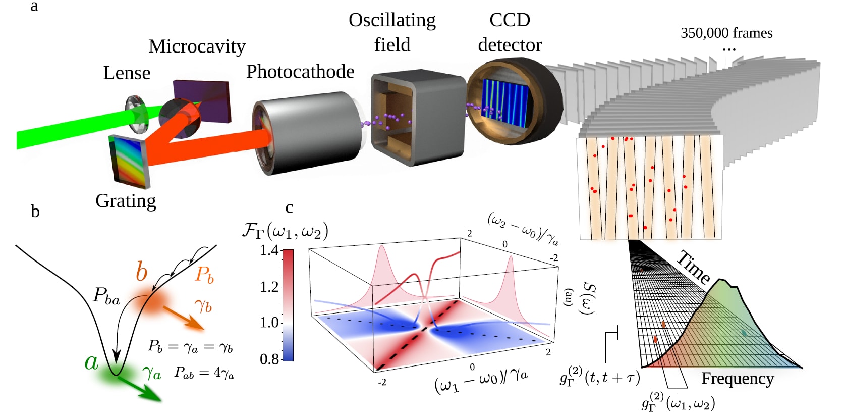
Figure 1: Principle and Setup of time- and frequency-resolved photon correlations. (a) Sketch of the experiment: the reflected light from a microcavity is dispersed onto a streak camera detecting at the single-photon level and stored in individual frames, whose post-processing allows to build photon-correlation landscapes (b) Sketch of the theory: a laser excites non-resonantly the lower polariton dispersion, creating a reservoir of hot excitons $b$ that condense into the ground state $a$ at the minimum of the branch. (c) Boson form factor $\mathcal{F}(\omega_{1},\omega_{2})$, i.e., time-integrated 2PS for the spontaneous emission of a coherent state with $g^{(2)}=1$, providing the backbone for the experiment. The diagonal and antidiagonal exhibit bunching and antibunching, respectively.

$$g_{\Gamma}^{(2)}(\omega_{1},t_{1};\omega_{2},t_{2})=\frac{\langle:\mathcal{T}\big{[}\prod_{i=1}^{2}\hat{E}_{\omega_{i},\Gamma}(t_{i})\hat{E}^{+}_{\omega_{i},\Gamma}(t_{i})\big{]}:\rangle}{\prod_{i=1}^{2}\langle\hat{E}_{\omega_{i},\Gamma}(t_{i})\hat{E}^{+}_{\omega_{i},\Gamma}(t_{i})\rangle},$$ (2)

where

$$\hat{E}_{\omega_{i},\Gamma}(t_{i})=\frac{\Gamma}{2}\int_{0}^{\infty}e^{-i\omega_{i}t}e^{-\Gamma t/2}\hat{E}(t_{i}-t)\,dt$$ (3)

is the electric field after passing through a filter with frequency component $\omega_{i}$ and width $\Gamma$ at time $t_{i}$, and $\mathcal{T}$, (resp. $:$) refers to time (resp. normal) ordering. Equation (24) provides the tendency of a correlated detection of one photon of frequency $\omega_{1}$ at time $t_{1}$ with another photon of frequency $\omega_{2}$ at time $t_{2}$. We consider here Lorentzian filters but this discussion applies to other types, such as square filters [16]. Frequency-resolved photon correlations are an increasingly popular experimental quantity, with already many measurements performed, although for fixed sets of frequencies, merely by inserting filters in the paths of a standard Hanbury Brown–Twiss setup [17, 18, 19, 20, 21, 22]. This measurement reveals its conceptual importance, however, when spanning over all possible combinations of energies, giving rise to a so-called “two-photon correlation spectrum” (2PS) [23, 24]. Considering the most common case of coincidences—$\tau=0$ in Eq. (1) and $t_{1}=t_{2}$ in Eq. (24)—one elevates in this way a single number, ${g^{(2)}_{0}\equiv g^{(2)}(t=0,\tau=0)}$, to a full landscape $g^{(2)}_{\Gamma}(\omega_{1},\omega_{2};\tau=0)$ of correlations. The quantity defined by such a landscape (the 2PS) acquires a fundamental meaning by revealing certain physical features [23, 24], in the same way that the normal spectrum is meaningful because its an observable that spans over a frequency range.

Results

In this work, we report the complete HBT effect extended to the full frequency-frequency map. We find that—in addition to the original observation of positive correlations for identical photons reported by the fathers of the effect and now routinely reproduced in a multitude of quantum-optical platforms worldwide—photons also manifest anticorrelations when they have different energies. Our results are a direct extension of the original HBT effect, that is the particular case of the diagonal on our 2PS. At such, it bears similar attributes as well as counter-intuitive consequences. Namely, two photons detected from two different sources manifest negative correlations if detected in different frequency windows (namely, on opposite sides of their mean energy) as compared to the unfiltered detection. If the sources are coherent, so that the unfiltered detection presents no correlation, the frequency-filtered photons exhibit anti-correlations: the detection of photons of a given color makes it less likely to detect photons of the other color. This behaviour is rooted in the bosonic fabric through what we will introduce as the “boson form factor”. Like the original HBT effect, our findings can be interpreted both from a quantum or a classical point of view, and being due to boson statistics, represent a fundamental backbone of every experiment involving frequency-resolved correlations. This result is therefore of deep relevance for any measurement of this kind, becoming of great interest in scenarios like the study of fluctuations [20] or the harvesting and use of quantum correlations that only emerge in the frequency-frequency domain [21, 22, 23, 25].

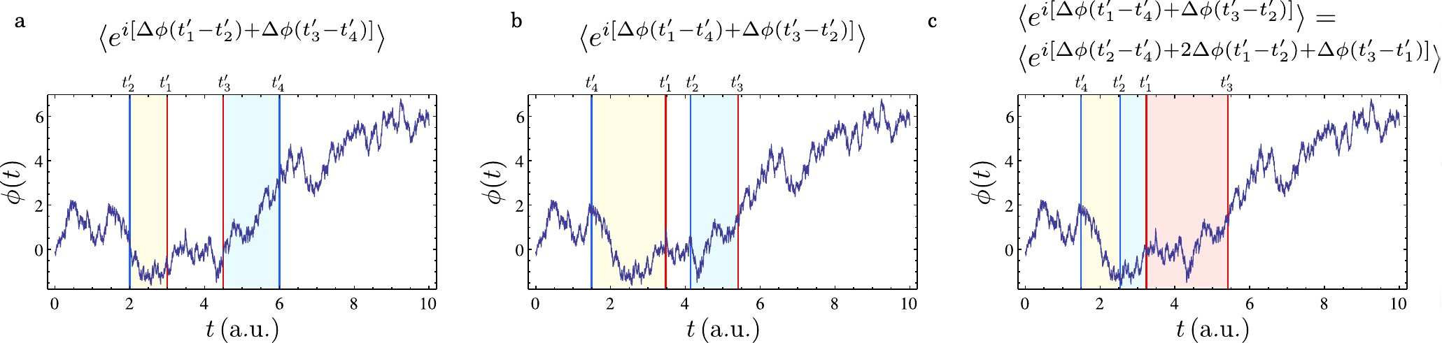
Figure 5: Examples of the possible integration domains for the fluctuating phase corresponding to three possible exponents that appear in the integrals: (a) Domain I, (b) Domain VIII and (c) Domain XI. In domains IX–XII, the exponent must be written as three phase differences to ensure they are statistically uncorrelated.

We have measured such anticorrelations between single photons emitted from a macroscopic out-of-equilibrium ensemble of exciton-polaritons pumped around the threshold of condensation. Polaritons are strongly-coupled light-matter bosonic particles in a semiconductor microcavity [26]. Such a source is more convenient than a laser because it is, for our purposes, essentially a laser with a broad linewidth, thereby allowing the spectral filtering. Besides, they have enjoyed thorough studies of their coherence properties, including at the quantum optical level [27, 28, 29]. The experiment is based on a streak camera setup that detects individual photons from the spontaneous emission of an ensemble of polaritons maintained in a non-equilibrium steady state under cw excitation. This is the first time that such a technique is used in the continuous pumping regime. The setup is sketched in Fig. 5a: light coming from the steady state of polaritons is dispersed by a spectrometer and is directed into the streak camera that is able to detect single photon events, as has already been demonstrated with standard photon correlations in time domain only, under pulsed excitation [30]. The sweeping in time and dispersion in energy allow the simultaneous recording of both the time and frequency of each detected photon in successive frames that are post-processed to calculate intensity correlations. Each frame includes several sweeps: in Fig. 1a, 8 sweeps per frame are shown as vertical orange stripes, with red dots indicating single photon events. Within each sweep, a time of 1536 ps is spanned in the vertical direction (3.2 ps per pixel), while the photon energy, obtained by coupling a spectrometer to the streak camera, is measured as horizontal pixel positions within each sweep (each sweep covers a total energy range of 456.7 $\mu\mathrm{eV}$, with 10.6 $\mu\mathrm{eV}$ per pixel). With the time- and energy-range used in this experiment, the overall temporal and energy resolution of the setup are of 10 ps and 70 $\mu\mathrm{eV}$, respectively. Correlation landscapes are obtained from coincidences between these clicks, with an average of $\approx 1.69$ clicks per sweep in a total of 350 000 frames. All the analysis is done with the raw data only: there is no normalisation and the correlations go to 1 at long time self-consistently.

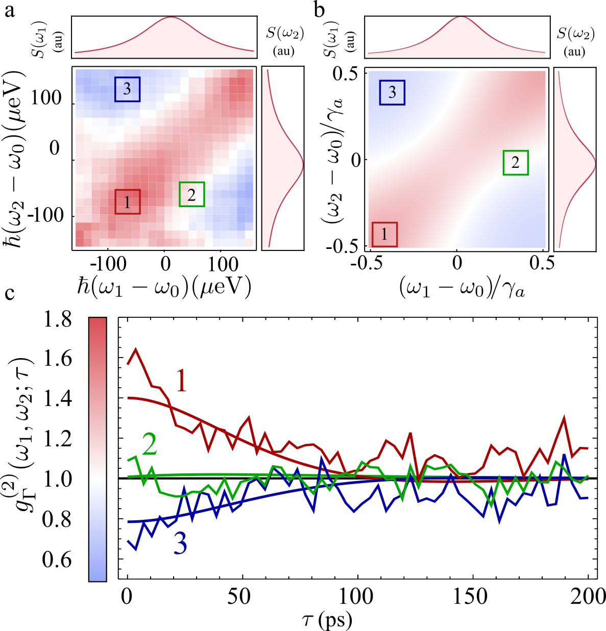
Figure 2: Two-photon correlations spectra. (a) Experimental observation of $g^{(2)}_{\Gamma}(\omega_{1},\omega_{2};0)$ for the spontaneous emission from a steady-state of polaritons. (b) Theoretical calculation of $g^{(2)}_{\Gamma}(\omega_{1},\omega_{2};0)$ from the model of condensation of polaritons sketched in Fig. 5b., showing a remarkable agreement. (c) Time-resolved correlation for the three regions marked in the colour map: (i) on the diagonal ($\omega_{1}=\omega_{2}$) exhibiting bunching, (ii) in the region of transition with no correlation, (iii) correlating opposing elbows, exhibiting antibunching.

A scheme of the emitter is shown in Fig. 5b: polaritons relax into the ground state from a reservoir of high energy polaritons injected by a cw off-resonant laser. The constant losses through the cavity mirror allow to study the steady-state correlations. Both the principle of the measurement and the technique are general and should allow, with optimisation, to shed new light in already well known systems in quantum optics, starting with the interesting non-classical properties displayed by quantum sources. The outstanding time resolution, which can be lower than 1 ps in a time window of 100 ps per sweep, makes this technique also of interest to study other phenomena such as spectral diffusion on fluctuating systems [20], promising to improve temporal precision by two orders of magnitude.

Figure 2a shows the experimental 2PS for the polariton state at $\tau=0$ together with the theoretical prediction, that is shown in Fig. 2b and was computed from the steady state emission of the model of condensation sketched in Fig. 5b using a master equation and the recently developed sensors method [31] (see Section IV of the Supplemental Material). Figure 2c depicts the temporal correlations for three points of the $(\omega_{1},\omega_{2})$–space, both for the experiment and the theoretical model, demonstrating an outstanding time precision in the scale of picoseconds. A clear evolution of the correlations from bunching ($g^{(2)}_{\Gamma}(\omega,\omega;0)\approx 1.5$ in region 1) to antibunching ($g^{(2)}_{\Gamma}(-\omega,\omega;0)\approx 0.7$ in region 3) is observed. In general, an excellent agreement with the theory is obtained, especially for the salient features which are diagonal bunching and antidiagonal antibunching.

Discussion

To the best of our knowledge, these features portray the first evidence of a HBT effect generalized to the full frequency-frequency domain. We now discuss these results in detail. Bunching in the diagonal line (corresponding to filters of equal frequency) is the well known feature of spectral filtering from a single peak [32]. From a classical point of view, this can be understood with the particular case of a quasi-monochromatic field $E(t)$ that has a finite bandwith given by a phase diffusion process:

$$E(t)=E_{0}e^{i[\omega_{0}t+\phi(t)]},$$ (4)

where $\phi(t)$ is a stochastic function that evolves, for instance, according to a random walk (see Fig. 3a). Such an errand phase allows for the line broadening. As is clear from Eq. (3), the frequency-filtered field is obtain by summing the field to itself at different times. If phase diffusion is present, this corresponds to the superposition of fields with random phases, which is analogous to the description of a thermal field. Consequently, such a superposition of fields of equal frequency but different phase produces interferences that wildly oscillate in a chaotic intensity profile, resulting in:

$$\frac{\langle{I_{\omega}}^{2}\rangle}{\langle I_{\omega}\rangle^{2}}>1.$$ (5)

This is well known textbook material [33]. Interpreted in terms of photons, the underlying particles thus tend to “clump” together, and increase the spacing between their arrival time, which gives rise to the bunching effect.

We have just seen how phase noise is thus converted into intensity noise by frequency-filtering (see Fig. 3b-c). In a related but subtler way—which is the novel feature that we report–such correlations can be negative when they involve different frequencies. This remains true at the single particle level, as is demonstrated by our experiment, with anticorrelations between photons of different colors. Since the effect is linked to the aforementioned conversion of phase noise into amplitude noise by filtering, we can keep the paradigmatic case of a quasi-monochromatic field, that has only phase noise. On physical grounds, one expects that a field with a stabilized Poynting vector (in which the uncertainty in the number of photons detected in a certain time window is given by the shot noise) cannot yield in average more photon counting events per unit time when spectrally resolved than it does without being frequency-filtered. Therefore, the detection of a clump of photons of some frequency in a small time window—in which photons are detected as random events prior filtering—must lower the probability of detecting photons at other, different frequencies, in order for the total rate of detected photons to be preserved. The anticorrelation we observe can therefore be interpreted as a consequence of energy conservation acting together with the HBT effect, that yields bunching of indistinguishable photons of equal frequencies. The photons on the detector, even if unrelated in the first place, cannot afford to remain so when frequency-filtered.

This argument is verified by explicit computation of Eq. (1) applied on the field Eq. (4), assuming random walk dynamics for the phase such that ${\langle e^{i[\phi(t)-\phi(t-\tau)]}\rangle}=e^{-\gamma|\tau|}$, ${\langle e^{2i[\phi(t)-\phi(t-\tau)]}\rangle=e^{-\gamma_{2}|\tau|}=e^{-4\gamma|\tau|}}$. The analytical expression for the frequency resolved correlation function at zero delay can be found exactly (the details of the calculation are given in Section I of the Supplemental Material):

$$g^{(2)}_{\Gamma}(\Delta_{1},\Delta_{2})=\frac{\left[\Delta_{1}^{2}+(\gamma+\Gamma/2)^{2}\right]\left[\Delta_{2}^{2}+(\gamma+\Gamma/2)^{2}\right]}{4(\gamma+\Gamma/2)^{2}}\times{}\\ \Re\left\{\frac{2(\gamma+3\Gamma/2)}{(\gamma+i\Delta_{2}+\Gamma/2)(\Delta_{1}^{2}+(\gamma+3\Gamma/2)^{2})}+\Gamma\left[f_{\Gamma}(\Delta_{2},\Delta_{12}^{-},\Delta_{2})\right.\right.+f_{\Gamma}(\Delta_{1},\Delta_{12}^{-},-\Delta_{2})+f_{\Gamma}(\Delta_{1},\Delta_{12}^{+}-i\gamma_{2},\Delta_{1})+\\ \left.\left.f_{\Gamma}(\Delta_{2},\Delta_{12}^{+}-i\gamma_{2},\Delta_{1})\right]+\left[\Delta_{1}\leftrightarrow\Delta_{2}\right]\vphantom{\frac{2(\gamma+3\lambda)}{(\Delta_{1}^{2}+(\gamma+3\lambda)^{2})}}\right\}$$ (6)

where $\Delta_{i}\equiv\omega_{i}-\omega_{0}$, $\Delta_{12}^{-}\equiv\Delta_{2}-\Delta_{1}$, $\Delta_{12}^{+}\equiv\Delta_{2}+\Delta_{1}$ and:

$$f_{\Gamma}(\omega_{1},\omega_{2},\omega_{3})=\frac{1}{(i\omega_{1}+\gamma+\Gamma/2)(i\omega_{2}+\Gamma)(i\omega_{3}+\gamma+3\Gamma/2)}\,.$$ (7)

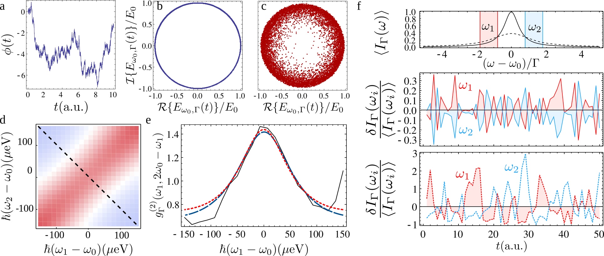
Figure 3: (a) The random-walk evolution of diffusing phase of a field $E(t)=E_{0}\exp{i[\omega_{0}t+\phi(t)]}$, with $\langle e^{i(\phi(t+\tau)-\phi(t))}\rangle=e^{-\gamma\tau}$ (b) $E(t)$ in phase space over different times. (c) Phase fluctuations are converted into intensity fluctuations after frequency filtering $E(t)$ (d) Fitting of the experimental 2PS by equation (6), with fitting parameters $\gamma\approx 193\,\mu\mathrm{eV}$, $\Gamma\approx 134\,\mu\mathrm{eV}$. The colorscale is that of Fig. 2. (e) 2PS along the dashed line in (d) for the experiment (straight, black), the fitting for the phase diffusing field (long dashed, blue) and the fitting of the form factor $\mathcal{F}_{\Gamma,\gamma,\gamma_{\phi}}$ (short-dashed, red). Despite not being an exact theoretical description for this experiment, the form factor agrees very well with the data for the parameters $\gamma\approx 99\,\mu\mathrm{eV}$, $\gamma_{\phi}\approx 440\,\mu\mathrm{eV}$, $\Gamma\approx 17\,\mu\mathrm{eV}$. (f) Fluctuations in the intensity of the filtered field $I_{\Gamma}(\omega_{i})=\langle I_{\Gamma}(\omega_{i})\rangle+\delta I_{\Gamma}(\omega_{i})$ for the two frequencies shown at the top panel and two values of $\gamma$, $\gamma\approx 8\times 10^{-3}\Gamma$ (solid lines, middle panel), and $\gamma\approx 0.8\,\Gamma$ (dashed lines, bottom panel). The corresponding values of $g^{(2)}(\omega_{1},\omega_{2})$ are 0.97 and 0.65 resp. In the middle-panel case, where $\Gamma\gg\gamma$, the anticorrelations in the noise become exact.

This expression reflects the same structure of correlations and anticorrelations observed in the experiment, as depicted in Fig. 3d-e, where it is shown to fit very well the experimental data. The main assumption behind this equation–that the unfiltered field has negligible amplitude fluctuations–is closely met in the experiment, in which the high coherence degree of the light emitted by the polaritons around the condensation threshold allows to unambiguously observe the anticorrelations. Just as the autocorrelations of Hanbury Brown for radio-waves of same frequencies (with no filtering), these anticorrelations of the filtered signal are obvious even to the naked eye, as can be seen in Fig. 3f, showing the intensity fluctuations of the simulated phase-diffusing field after frequency filtering. Surprisingly, such anticorrelations in the noise can even become exact, when the filter linewidth becomes much larger than the natural linewidth of the field ($\Gamma\gg\gamma$). This is proved in Section I of the Supplemental Material. In this case, although $g^{(2)}(\omega_{1},\omega_{2})$ gets closer to one (converging to the “unfiltered” result), the smaller fluctuations $\delta I_{\Gamma}(\omega_{i})$ around the mean value $I_{\Gamma}(\omega_{i})=\langle I_{\Gamma}(\omega_{i})\rangle+\delta I_{\Gamma}(\omega_{i})$ tend to become perfectly anticorrelated for frequencies in opposite sides of the spectrum, $\delta I_{\Gamma}(\omega_{0}-\omega)\approx-\delta I_{\Gamma}(\omega_{0}+\omega)$, as can be observed in the middle panel of Fig. 3f.

Describing this effect from the quantum/particle point of view poses more difficulties, since the 2PS is a dynamical observable and one cannot attribute a value of $g^{(2)}_{0}$ with frequency-filtering to a given quantum state without also including information about the dynamics, unlike the case without frequency-filtering where the knowledge of the diagonal elements of the density matrix is sufficient. Such differences are discussed from a more technical point of view in Section II of the Supplemental Material. This makes the formulation of a general statement a complicated task. We consider for that purpose a simple situation in which an arbitrary quantum state given by the density matrix $\rho(0)$ is left to decay from a source to a continuum of modes under spontaneous emission with a rate $\gamma_{a}$ and also with a pure dephasing rate $\gamma_{\phi}$, thus eliminating every possible dynamics except the essential one that brings photons from the source to the detector and some dephasing mechanism. Therefore, the resulting master equation is given by $\partial_{t}\rho=\left[\frac{\gamma_{a}}{2}\mathcal{L}_{a}+\frac{\gamma_{\phi}}{2}\mathcal{L}_{a^{\dagger}a}\right]\rho$, where $\mathcal{L}_{O}$ denotes the usual Lindblad term, $\mathcal{L}_{O}\rho=2O\rho O^{\dagger}-O^{\dagger}O\rho-\rho O^{\dagger}O$. We have obtained the analytical expression of the normalized correlation for the counts at different frequencies integrated in time, which takes the form:

$$g^{(2)}_{\Gamma}(\omega_{1},\omega_{2})=g_{0}^{(2)}\mathcal{F}_{\Gamma,\gamma,\gamma_{\phi}}(\omega_{1},\omega_{2})$$ (8)

with $g_{0}^{(2)}$ the zero delay second-order correlation function of the initial state and $\mathcal{F}_{\Gamma,\gamma,\gamma_{\phi}}(\omega_{1},\omega_{2})$ a form factor (see Fig. 5c, Fig. 3e and Section III of the Supplemental Material for the analytical expression), independent of this state, that reproduces exactly the features observed in the experiment and therefore captures the essence of this extension of the HBT effect. The wide range of frequencies used in Figure 1c serves to illustrate the non trivial shape of the anticorrelations along the antidiagonal line $(\omega,-\omega)$, featuring a minimum approximately at the point where the total filtered intensity is maximum without a considerable overlapping of the filters. It follows from the arguments above that some dephasing mechanism is an essential ingredient for the manifestation of the phenomenon (as it is for the standard HBT effect). This is directly implied in the classical picture and consistently confirmed in the quantum calculation, since when the dephasing rate $\gamma_{\phi}$ is equal to zero, $\mathcal{F}_{\Gamma,\gamma,\gamma_{\phi}}(\omega_{1},\omega_{2})$ is equal to one, and therefore featureless. This also explains why the coherent part of the resonance fluorescence spectrum, not subjected to dephasing, does not present this features while the incoherent part does (see Fig. 7 of [23]). Consistently with the classical analysis based on a stochastic field (4), the quantum calculation shows that when the unfiltered field has no intensity fluctuations $g_{0}^{(2)}=1$, the filtered field displays anticorrelations. Both general analysis (classical and quantum), together with the experiment and the theoretical characterization of the steady state emission of our specific system, complete our description of the effect.

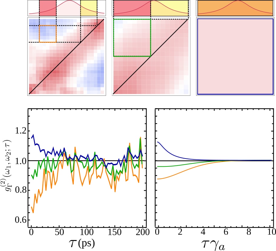
Figure 4: Two-photon correlation landscapes $g^{(2)}(\omega_{1},\omega_{2};0)$ as a function of the filter width, from a fraction of the peak, 74.1 $\mu eV$ (left), roughly half-peak width, 158.8 $\mu eV$ (center), to full-peak filtering, corresponding to standard auto-correlations. The position of the two filters is shown explicitly on the spectral line as the red and yellow windows (orange when overlapping). Bottom left and right panels describe the experiment and the theory from the condensation model, respectively.

Another fundamental feature of the theory is that correlations depend on the frequency windows that select which photons are correlated. Smaller windows lead to stronger correlations but, again, at the price of a smaller signal. While it does not correspond exactly to a change in the width of the filter, the effect is neatly illustrated by changing the number of pixels of the streak camera that we associate to a given frequency. In Fig. 3f, we show the dependence of the 2PS on the size of the frequency windows for a point that features antibunching. When the frequency window is very large, $\Gamma\gg\gamma_{a}$, both the experimental and theoretical $g^{(2)}_{\Gamma}(\omega_{1},\omega_{2};\tau)$ recover as expected the results of standard photon correlations which has always been reported to be larger than 1 for this kind of systems [34, 35, 36]. As the size of the frequency window decreases, the system shows a transition from bunching to antibunching, demonstrating how the statistics of coloured photons can be easily tuned externally.

These results, that generalize the Hanbury Brown–Twiss effect to exhibit correlations of different types depending on the energies— are of fundamental interest, but are also of technological importance. Indeed, the main observable—the frequency-resolved correlation function—is of increasing importance in quantum-optical technologies. Spectrally-resolved photon counting measurements can be a useful tool in non-linear spectroscopy, able to measure ultrafast dynamics [37]. Applications for measuring fluctuations through detection of single photons in time and frequency with picosecond resolution in spectral diffusion problems [20] should also benefit from both our findings and experimental setup. Our results and methods are also of importance for the study of quantum systems with more complex dynamics beyond merely spontaneous emission and dephasing [31, 23]. In cases of strongly correlated emission, virtual processes [38, 39] result in 2PS with strong geometric features, such as antidiagonals or circles of correlations [23, 24]. Such rich landscapes of photon correlations, inherited from the system’s quantum dynamics, are otherwise lost by disregarding the frequencies. The results presented here provide the backbone for more general schemes that, for practical purposes such as distillation [40] or Purcell enhancement [38, 41], can be used to power quantum technology. Like Purcell did in his pioneering interpretation of the HBT effect [7], we conjecture a counterpart for fermion correlations, namely, with an orthogonal profile: antibunching on the diagonal and bunching on the antidiagonal; this question, that could be investigated for instance in transport experiments with electrons [42], is however outside the scope of this text and its field of research, and is left to experimental and theoretical colleagues in other disciplines.

Conclusion

We report the measurement of anticorrelations between individual photons emitted from a ensemble of polaritons under continuous pumping. We have demonstrated that this phenomenon is a fundamental result that generalizes the Hanbury Brown–Twiss effect for color correlations, and is therefore linked to the bosonic nature of photons. We have introduced a novel experimental technique that allows to measure correlations in time and energy between individual photons, demonstrating that both the concept and technique of color correlations are sound and ripe to be deployed in a large range of quantum optical systems, with prospects of accessing further classes of quantum correlations [43, 44], optimising those already known [40, 39], or analysing problems such as spectral diffusion at new levels of precision [20].

Supplementary Material

Materials

The sample is a high quality factor GaAs/AlGaAs planar cavity containing 12 GaAs quantum wells placed at three anti-node positions of the electrical field. The front (back) mirror consists of 34 (40) pairs of AlAs/Al0.2Ga0.8As layers. It is pumped at normal incidence and non-resonantly with a single-mode laser at a wavelength of 752 $\mu\mathrm{m}$. Thanks to a double electronic synchronization, an additional “slow” sweeping in time is performed also in the horizontal direction, thus recording multiple sweeps per frame: in this way the number of events detected in each frame is increased of about one order of magnitude, allowing the detection of a large statistics of events in a relatively short measurement time, going beyond the limits imposed by the electronics speed of CCD devices.

I. Calculation of $g^{(2)}_{\Gamma}(\omega_{1},\omega_{2},\tau)$ for a phase diffusing field

In this section, we give the details of the calculation of the frequency-resolved correlation function for a classical stochastic field. Such a phase-diffusing field but with otherwise stabilized intensity (describing a coherent field) reads:

$$E(t)=E_{0}e^{-i[\omega_{0}t+\phi(t)]}\,,$$ (9)

where the phase is a random variable that is considered to undergo a random walk evolution. The phase difference $\Delta\phi(\tau)=\phi(t+\tau)-\phi(t)$ has the following properties:

$$\langle\Delta\phi(\tau)\rangle = 0\,,$$

$$\langle\Delta\phi(\tau)^{2}\rangle = 2\gamma_{1}|\tau|\,,$$

$$\langle e^{i[\phi(t)-\phi(t-\tau)]}\rangle = e^{-\gamma_{1}|\tau|}\,,$$

$$\langle e^{2i[\phi(t)-\phi(t-\tau)]}\rangle = e^{-\gamma_{2}|\tau|}\,.$$ (10)

In the case of a phase diffusing field, the fourth orther correlation constant $\gamma_{2}$ is given by $\gamma_{2}=4\gamma_{1}$. However, we keep $\gamma_{2}$ in the expressions to account for other possible models of phase noise, like the phase-jump model, in which $\gamma_{2}=\gamma_{1}$ [45]. These properties allow us to compute the frequency resolved second-order correlation function:

$$g^{(2)}_{\Gamma}(\omega_{1},\omega_{2},\tau)=\frac{\langle E_{\omega_{2},\Gamma}^{+}(t+\tau)E_{\omega_{2},\Gamma}(t+\tau)E_{\omega_{1},\Gamma}^{+}(t)E_{\omega_{1},\Gamma}(t)\rangle}{\langle E_{\omega_{2},\Gamma}^{+}(t+\tau)E_{\omega_{2},\Gamma}(t+\tau)\rangle\langle E_{\omega_{1},\Gamma}^{+}(t)E_{\omega_{1},\Gamma}(t)\rangle},$$ (11)

where $E_{\omega,\Gamma}(t)$ describes the field filtered at frequency $\omega$ with a filter linewidth $\Gamma$:

$$E_{\omega,\Gamma}(t)=\frac{\Gamma}{2}\int_{0}^{\infty}e^{-i\omega t^{\prime}}e^{-\Gamma\,t^{\prime}/2}E(t-t^{\prime})\,dt^{\prime}.$$ (12)

This calculation is done with the properties listed in Eq. (10). The numerator of Eq. (11), that we denote $G^{(2)}_{\Gamma}(\omega_{1},\omega_{2},\tau)$, is given by the following quadruple integral:

$$G^{(2)}_{\Gamma}(\omega_{1},\omega_{2},\tau)=\left(\frac{\Gamma}{2}\right)^{4}\int_{0}^{\infty}\prod_{i=1}^{4}dt_{i}\,e^{i\omega_{1}(t_{2}-t_{1})}e^{i\omega_{2}(t_{4}-t_{3})}e^{-\Gamma(t_{1}+t_{2}+t_{3}+t_{4})/2}\langle E(t-t_{3}+\tau)E^{*}(t-t_{4}+\tau)E(t-t_{1})E^{*}(t-t_{2})\rangle\\ =E_{0}^{4}\left(\frac{\Gamma}{2}\right)^{4}\int_{0}^{\infty}\prod_{i=1}^{4}dt_{i}\,e^{-i\Delta_{1}(t_{2}-t_{1})-i\Delta_{2}(t_{3}-t_{4})}e^{-\Gamma(t_{1}+t_{2}+t_{3}+t_{4})/2}\langle e^{-i[\phi(t-t_{1})-\phi(t-t_{2})+\phi(t-t_{3}+\tau)-\phi(t-t_{4}+\tau)]}\rangle\,,$$ (13)

where $\Delta_{i}\equiv\omega_{0}-\omega_{i}$. Defining $t_{1}^{\prime}\equiv t-t_{1}$, $t_{2}^{\prime}\equiv t-t_{2}$, $t_{3}^{\prime}\equiv t-t_{3}+\tau$ and $t_{4}^{\prime}\equiv t-t_{4}+\tau$, the statistical average in the last line of (13) takes the form $\langle e^{i[\phi(t_{1}^{\prime})-\phi(t_{2}^{\prime})+\phi(t_{3}^{\prime})-\phi(t_{4}^{\prime})]}\rangle$. The exponent can be written in term of phase differences $\Delta\phi(\tau)$ in two possible ways, $\langle e^{i[\Delta\phi(t_{1}^{\prime}-t_{2}^{\prime})+\Delta\phi(t_{3}^{\prime}-t_{4}^{\prime})]}\rangle$ or $\langle e^{i[\Delta\phi(t_{1}^{\prime}-t_{4}^{\prime})+\Delta\phi(t_{3}^{\prime}-t_{2}^{\prime})]}\rangle$. For a given set of values for $t_{1}^{\prime}$, $t_{2}^{\prime}$, $t_{3}^{\prime}$ and $t_{4}^{\prime}$, the choice between both options must be made such that the two $\Delta\phi$ are defined in non-overlapping time intervals, making them statistically independent. This allows to factorize the exponential and use Eq. (10) to evaluate the statistical averages. Figure 5 depicts the three possible configurations that exist depending on the values of $t_{i}^{\prime}$. Panel c shows the particular case $t^{\prime}_{4},t_{2}^{\prime}<t_{1}^{\prime},t_{3}^{\prime}$ that requires the introduction of a third time interval to avoid overlapping; this is the case that will invoke the last equation in Eq. (10), involving the fourth order correlation constant $\gamma_{2}$. Since the integrand has to be written differently depending on the values of the $t_{i}^{\prime}$, one needs to split the integral in the 24 possible domains. Half of these integrals are the complex conjugate of the other half, yielding 12 independent terms, defined in the domains:

$$\mathrm{I:} t_{2}^{\prime}<t_{1}^{\prime}<t_{3}^{\prime}<t_{4}^{\prime}\quad\stackrel{{\scriptstyle*}}{{\leftrightarrow}}\quad t_{1}^{\prime}<t_{2}^{\prime}<t_{4}^{\prime}<t_{3}^{\prime}\,,$$

$$\mathrm{II:} t_{2}^{\prime}<t_{3}^{\prime}<t_{1}^{\prime}<t_{4}^{\prime}\quad\stackrel{{\scriptstyle*}}{{\leftrightarrow}}\quad t_{1}^{\prime}<t_{4}^{\prime}<t_{2}^{\prime}<t_{3}^{\prime}\,,$$

$$\mathrm{III:} t_{4}^{\prime}<t_{3}^{\prime}<t_{1}^{\prime}<t_{2}^{\prime}\quad\stackrel{{\scriptstyle*}}{{\leftrightarrow}}\quad t_{3}^{\prime}<t_{4}^{\prime}<t_{2}^{\prime}<t_{1}^{\prime}\,,$$

$$\mathrm{IV:} t_{4}^{\prime}<t_{1}^{\prime}<t_{3}^{\prime}<t_{2}^{\prime}\quad\stackrel{{\scriptstyle*}}{{\leftrightarrow}}\quad t_{3}^{\prime}<t_{2}^{\prime}<t_{4}^{\prime}<t_{1}^{\prime}\,,$$

$$\mathrm{V:} t_{2}^{\prime}<t_{1}^{\prime}<t_{4}^{\prime}<t_{3}^{\prime}\quad\stackrel{{\scriptstyle*}}{{\leftrightarrow}}\quad t_{1}^{\prime}<t_{2}^{\prime}<t_{3}^{\prime}<t_{4}^{\prime}\,,$$

$$\mathrm{VI:} t_{2}^{\prime}<t_{3}^{\prime}<t_{4}^{\prime}<t_{1}^{\prime}\quad\stackrel{{\scriptstyle*}}{{\leftrightarrow}}\quad t_{1}^{\prime}<t_{4}^{\prime}<t_{3}^{\prime}<t_{2}^{\prime}\,,$$

$$\mathrm{VII:} t_{4}^{\prime}<t_{3}^{\prime}<t_{2}^{\prime}<t_{1}^{\prime}\quad\stackrel{{\scriptstyle*}}{{\leftrightarrow}}\quad t_{3}^{\prime}<t_{4}^{\prime}<t_{1}^{\prime}<t_{2}^{\prime}\,,$$

$$\mathrm{VIII:} t_{4}^{\prime}<t_{1}^{\prime}<t_{2}^{\prime}<t_{3}^{\prime}\quad\stackrel{{\scriptstyle*}}{{\leftrightarrow}}\quad t_{3}^{\prime}<t_{2}^{\prime}<t_{1}^{\prime}<t_{4}^{\prime}\,,$$

$$\mathrm{IX:} t_{2}^{\prime}<t_{4}^{\prime}<t_{1}^{\prime}<t_{3}^{\prime}\quad\stackrel{{\scriptstyle*}}{{\leftrightarrow}}\quad t_{1}^{\prime}<t_{3}^{\prime}<t_{2}^{\prime}<t_{4}^{\prime}\,,$$

$$\mathrm{X:} t_{2}^{\prime}<t_{4}^{\prime}<t_{3}^{\prime}<t_{1}^{\prime}\quad\stackrel{{\scriptstyle*}}{{\leftrightarrow}}\quad t_{1}^{\prime}<t_{3}^{\prime}<t_{2}^{\prime}<t_{4}^{\prime}\,,$$

$$\mathrm{XI:} t_{4}^{\prime}<t_{2}^{\prime}<t_{1}^{\prime}<t_{3}^{\prime}\quad\stackrel{{\scriptstyle*}}{{\leftrightarrow}}\quad t_{3}^{\prime}<t_{1}^{\prime}<t_{2}^{\prime}<t_{4}^{\prime}\,,$$

$$\mathrm{XII:} t_{4}^{\prime}<t_{2}^{\prime}<t_{3}^{\prime}<t_{1}^{\prime}\quad\stackrel{{\scriptstyle*}}{{\leftrightarrow}}\quad t_{3}^{\prime}<t_{1}^{\prime}<t_{4}^{\prime}<t_{2}^{\prime}\,.$$ (14)

By denoting the non-overlapping time differences as $\tau_{i}$ and making a change of variables, the corresponding integrals take the form:

$$I_{\mathrm{I}} = C\int_{0}^{\infty}dt_{2}\int_{t_{2}}^{0}d\tau_{1}\int_{0}^{t_{2}-\tau_{1}+\tau}\kern-14.22636ptdt_{3}\int_{t_{3}}^{0}d\tau_{2}\,e^{i(\Delta_{2}\tau_{2}-\Delta_{1}\tau_{1})}e^{-\Gamma(2t_{2}+2t_{3}-\tau_{1}-\tau_{2})/2-\gamma(\tau_{1}+\tau_{2})},$$

$$I_{\mathrm{II}} = C\int_{0}^{\infty}dt_{2}\int_{t_{2}}^{0}d\tau_{1}\int_{0}^{t_{2}-\tau_{1}}\kern-11.38092ptdt_{1}\int_{t_{1}+\tau}^{0}d\tau_{2}\,e^{i\Delta_{1}(t_{1}-t_{2})+i\Delta_{2}(\tau_{2}-\tau_{1}+t_{2}-t_{1})}e^{-\Gamma(2t_{2}-\tau_{1}+2t_{1}-\tau_{2}+2\tau)/2-\gamma(\tau_{1}+\tau_{2})},$$

$$I_{\mathrm{III}} = C\int_{\tau}^{\infty}dt_{4}\int_{t_{4}-\tau}^{0}d\tau_{1}\int_{0}^{t_{4}-\tau_{1}-\tau}\kern-14.22636ptdt_{1}\int_{t_{1}}^{0}d\tau_{2}\,e^{i(\Delta_{1}\tau_{2}-\Delta_{2}\tau_{1}}e^{-\Gamma(2t_{4}+2t_{1}-\tau_{1}-\tau_{2})/2-\gamma(\tau_{1}+\tau_{2})},$$

$$I_{\mathrm{IV}} = C\int_{\tau}^{\infty}dt_{4}\int_{t_{4}-\tau}^{0}d\tau_{1}\int_{\tau}^{t_{4}-\tau_{1}}\kern-14.22636ptdt_{3}\int_{t_{3}-\tau}^{0}d\tau_{2}\,e^{i\Delta_{2}(t_{3}-t_{4})+i\Delta_{1}(\tau_{2}-\tau_{1}+t_{4}-t_{3})}e^{-\Gamma(2t_{4}+2t_{3}-\tau_{1}-\tau_{2}-2\tau)/2-\gamma(\tau_{1}+\tau_{2})},$$

$$I_{\mathrm{V}} = C\int_{0}^{\infty}dt_{2}\int_{t_{2}}^{0}d\tau_{1}\int_{0}^{t_{2}-\tau_{1}+\tau}\kern-17.07182ptdt_{4}\int_{t_{4}}^{0}d\tau_{2}\,e^{-i(\Delta_{1}\tau_{1}+\Delta_{2}\tau_{2})}e^{-\Gamma(2t_{2}+2t_{4}-\tau_{1}-\tau_{2})/2-\gamma(\tau_{1}+\tau_{2})},$$

$$I_{\mathrm{VI}} = C\int_{0}^{\infty}dt_{2}\int_{t_{2}}^{0}d\tau_{1}\int_{\tau}^{t_{2}-\tau_{1}+\tau}\kern-17.07182ptdt_{4}\int_{t_{4}-\tau}^{0}d\tau_{2}\,e^{-i\Delta_{1}(t_{2}-t_{4}+\tau+\tau_{2})-i\Delta_{2}(t_{4}-t_{2}-\tau+\tau_{1})}e^{-\Gamma(2t_{2}+2t_{4}-\tau_{1}-\tau_{2})/2-\gamma(\tau_{1}+\tau_{2})},$$

$$I_{\mathrm{VII}} = C\int_{\tau}^{\infty}dt_{4}\int_{t_{4}-\tau}^{0}d\tau_{1}\int_{0}^{t_{4}-\tau_{1}-\tau}\kern-14.22636ptdt_{2}\int_{t_{2}}^{0}d\tau_{2}\,e^{-i\Delta_{1}\tau_{2}-i\Delta_{2}\tau_{1}}e^{-\Gamma(2t_{4}+2t_{2}-\tau_{1}-\tau_{2})/2-\gamma(\tau_{1}+\tau_{2})},$$

$$I_{\mathrm{VIII}} = C\int_{\tau}^{\infty}dt_{4}\int_{t_{4}-\tau}^{0}d\tau_{1}\int_{0}^{t_{4}-\tau_{1}-\tau}\kern-14.22636ptdt_{2}\int_{t_{2}+\tau}^{0}d\tau_{2}\,e^{-i\Delta_{1}(t_{2}-t_{4}+\tau+\tau_{1})-i\Delta_{2}(t_{4}-t_{2}-\tau+\tau_{2})}e^{-\Gamma(2t_{4}+2t_{2}-\tau_{1}-\tau_{2})/2-\gamma(\tau_{1}+\tau_{2})},$$

$$I_{\mathrm{IX}} = -C\int_{0}^{\infty}dt_{2}\int_{t_{2}}^{0}d\tau_{1}\int_{t_{2}-\tau_{1}}^{0}\kern-14.22636ptd\tau_{2}\int_{t_{2}-\tau_{1}-\tau_{2}+\tau}^{0}\kern-28.45274ptd\tau_{3}\,e^{-i\Delta_{1}(\tau_{1}+\tau_{2})-i\Delta_{2}(\tau_{2}+\tau_{3})}e^{-\Gamma(4t_{2}-3\tau_{1}-2\tau_{2}-\tau_{3}+2\tau)/2-\gamma(\tau_{1}+\tau_{3})-\gamma_{2}\tau_{2}},$$

$$I_{\mathrm{X}} = -C\int_{0}^{\infty}dt_{2}\int_{t_{2}}^{0}d\tau_{1}\int_{t_{2}-\tau_{1}}^{0}d\tau_{2}\int_{t_{2}-\tau_{1}-\tau_{2}}^{0}\kern-19.91684ptd\tau_{3}\,e^{-i\Delta_{1}(\tau_{1}+\tau_{2}+\tau_{3})-i\Delta_{2}\tau_{2}}e^{-\Gamma(4t_{2}+2\tau-3\tau_{1}-2\tau_{2}-\tau_{3})/2-\gamma(\tau_{1}+\tau_{3})-\gamma_{2}\tau_{2}},$$

$$I_{\mathrm{XI}} = -C\int_{\tau}^{\infty}dt_{4}\int_{t_{4}-\tau}^{0}d\tau_{1}\int_{t_{4}-\tau-\tau_{1}}^{0}\kern-14.22636ptd\tau_{2}\int_{t_{4}-\tau_{1}-\tau_{2}}^{0}\kern-19.91684ptd\tau_{3}\,e^{-i\Delta_{1}\tau_{2}-i\Delta_{2}(\tau_{1}+\tau_{2}+\tau_{3})}e^{-\Gamma(4t_{4}-2\tau-3\tau_{1}-2\tau_{2}-\tau_{3})/2-\gamma(\tau_{1}+\tau_{3})-\gamma_{2}\tau_{2}},$$

$$I_{\mathrm{XII}} = -C\int_{\tau}^{\infty}dt_{4}\int_{t_{4}-\tau}^{0}d\tau_{1}\int_{t_{4}-\tau-\tau_{1}}^{0}\kern-14.22636ptd\tau_{2}\int_{t_{4}-\tau_{1}-\tau_{2}-\tau}^{0}\kern-28.45274ptd\tau_{3}\,e^{-i\Delta_{1}(\tau_{2}+\tau_{3})-i\Delta_{2}(\tau_{1}+\tau_{2})}e^{-\Gamma(4t_{4}-2\tau-3\tau_{1}-2\tau_{2}-\tau_{3})/2-\gamma(\tau_{1}+\tau_{3})-\gamma_{2}\tau_{2}},$$

with $C=E_{0}^{4}\left(\frac{\Gamma}{2}\right)^{4}$.

Finally, $G^{(2)}_{\Gamma}(\omega_{1},\omega_{2},\tau)$ is given by:

$$G^{(2)}_{\Gamma}(\omega_{1},\omega_{2},\tau)=2\mathrm{Re}\sum_{i=\mathrm{I}}^{\mathrm{XII}}I_{i}={}$$ (16)

$$\frac{1}{16}\Gamma^{2}\mathrm{Re}\left\{\frac{2ie^{\tau\left(-\gamma-\frac{\Gamma}{2}-i\Delta_{2}\right)}\left(\gamma_{2}\left(\frac{i\Gamma}{2}+2\Delta_{1}-\Delta_{2}\right)+\left(\frac{\Gamma}{2}+i\Delta_{1}\right)\left(-i\Gamma+\Delta_{1}+\Delta_{2}\right)+\gamma\left(-3i\Gamma-i\gamma_{2}-\Delta_{1}+3\Delta_{2}\right)\right)\Gamma^{2}}{\left(\gamma+\frac{\Gamma}{2}+i\Delta_{1}\right)\left(\gamma-\frac{\Gamma}{2}+i\Delta_{2}\right)\left(\gamma+\frac{\Gamma}{2}+i\Delta_{2}\right)\left(\gamma+\frac{3\Gamma}{2}+i\Delta_{2}\right)\left(-i\Gamma-\Delta_{1}+\Delta_{2}\right)\left(-i\Gamma-i\gamma_{2}+\Delta_{1}+\Delta_{2}\right)}\right.$$

$$+ \frac{2e^{\tau\left(-\gamma-\frac{\Gamma}{2}+i\Delta_{2}\right)}\left(\gamma-\frac{\Gamma}{2}-i\Delta_{1}\right)\Gamma^{2}}{\left(\gamma+\frac{\Gamma}{2}+i\Delta_{1}\right)\left(\gamma+\frac{\Gamma}{2}-i\Delta_{2}\right)\left(\gamma+\frac{3\Gamma}{2}-i\Delta_{2}\right)\left(i\gamma-\frac{i\Gamma}{2}+\Delta_{2}\right)\left(i\Gamma-\Delta_{1}+\Delta_{2}\right)}$$

$$+ \frac{e^{-\Gamma\tau}\left(-\Gamma^{3}-\frac{1}{2}\left(4\gamma+i\left(3\Delta_{1}+\Delta_{2}\right)\right)\Gamma^{2}+\frac{1}{2}\left(\Delta_{1}-\Delta_{2}\right)\left(2i\gamma-3i\gamma_{2}+\Delta_{1}+3\Delta_{2}\right)\Gamma+\left(\Delta_{1}-\Delta_{2}\right)\left(\gamma+i\Delta_{2}\right)\left(-i\gamma_{2}+\Delta_{1}+\Delta_{2}\right)\right)}{\left(\gamma+\frac{\Gamma}{2}+i\Delta_{1}\right)\left(\gamma-\frac{\Gamma}{2}+i\Delta_{2}\right)\left(\gamma+\frac{\Gamma}{2}+i\Delta_{2}\right)\left(-i\Gamma-\Delta_{1}+\Delta_{2}\right)\left(-i\Gamma-i\gamma_{2}+\Delta_{1}+\Delta_{2}\right)}$$

$$+ e^{-\Gamma\tau}\left[\frac{2\left(\gamma+\frac{3\Gamma}{2}\right)}{\left(\left(\gamma+\frac{3\Gamma}{2}\right)^{2}+\Delta_{1}^{2}\right)\left(\gamma+\frac{\Gamma}{2}+i\Delta_{2}\right)}+\frac{i\Gamma}{\left(\gamma+\frac{3\Gamma}{2}-i\Delta_{1}\right)\left(i\Gamma+\Delta_{1}-\Delta_{2}\right)\left(\gamma+\frac{\Gamma}{2}+i\Delta_{2}\right)}\right.$$

$$+ \frac{\Gamma}{\left(\gamma+\frac{\Gamma}{2}+i\Delta_{1}\right)\left(\gamma+\frac{3\Gamma}{2}+i\Delta_{1}\right)\left(\Gamma+\gamma_{2}+i\left(\Delta_{1}+\Delta_{2}\right)\right)}+\frac{\Gamma}{\left(\gamma+\frac{3\Gamma}{2}+i\Delta_{1}\right)\left(\gamma+\frac{\Gamma}{2}+i\Delta_{2}\right)\left(\Gamma+\gamma_{2}+i\left(\Delta_{1}+\Delta_{2}\right)\right)}$$

$$+ \left.\frac{\Gamma}{\left(\gamma+\frac{\Gamma}{2}+i\Delta_{1}\right)\left(\gamma+\frac{3\Gamma}{2}+i\Delta_{1}\right)\left(\Gamma+i\left(\Delta_{1}-\Delta_{2}\right)\right)}\right]+\frac{2}{\left(\gamma+\frac{\Gamma}{2}+i\Delta_{1}\right)\left(\gamma+\frac{\Gamma}{2}-i\Delta_{2}\right)}+\frac{2}{\left(\gamma+\frac{\Gamma}{2}+i\Delta_{1}\right)\left(\gamma+\frac{\Gamma}{2}+i\Delta_{2}\right)}$$

$$+ \left.\frac{e^{-\Gamma\tau}\left(\Delta_{2}-\Delta_{1}\right)}{\left(\gamma+\frac{\Gamma}{2}+i\Delta_{1}\right)\left(-\gamma+\frac{\Gamma}{2}+i\Delta_{2}\right)\left(i\Gamma-\Delta_{1}+\Delta_{2}\right)}\right\}\,.$$

On the other hand, the denominator in Eq. (11) consists of the product of the mean intensities of the two filtered fields. This mean intensity is readily given by:

$$\langle E^{+}_{\omega_{i},\Gamma}(t)E_{\omega_{i},\Gamma}(t)\rangle=\langle I_{\omega_{i},\Gamma}(t)\rangle=E_{0}^{2}\frac{\Gamma^{2}}{4}\left(\int_{0}^{\infty}dt_{1}\int_{0}^{t_{1}}dt_{2}\,e^{i\Delta_{i}(t_{1}-t_{2})-\Gamma(t_{1}+t_{2})/2-\gamma(t_{1}-t_{2})}+\right.$$

$$\left.\int_{0}^{\infty}dt_{2}\int_{0}^{t_{2}}dt_{1}\,e^{i\Delta_{i}(t_{1}-t_{2})-\Gamma(t_{1}+t_{2})/2-\gamma(t_{2}-t_{1})}\right)$$

$$=E_{0}^{2}\frac{\Gamma^{2}}{2}\mathrm{Re}\int_{0}^{\infty}dt_{1}\int_{0}^{t_{1}}dt_{2}\,e^{(i\Delta_{i}-\gamma)(t_{1}-t_{2})-\Gamma(t_{1}+t_{2})/2}=E_{0}^{2}\frac{\Gamma}{2}\frac{\gamma+\Gamma/2}{\Delta_{i}^{2}+(\gamma+\Gamma/2)^{2}}\,.$$ (17)

Normalizing the expression of $G^{(2)}_{\Gamma}(\omega_{1},\omega_{2},\tau)$ given in Eq. (16) by the intensities in Eq. (17), we obtain the final expression for $g^{(2)}_{\Gamma}(\omega_{1},\omega_{2},\tau)$. At $\tau=0$, this expression takes the more compact form presented in the main text.

An interesting limit, reported in Fig. 3f of the main text, occurs when the filter linewidth is much larger than the natural linewidth of the field, $\Gamma\gg\gamma$. The intensity of the filtered field is then given by:

$$I_{\omega_{i},\Gamma}(t) = E_{0}^{2}\frac{\Gamma^{2}}{2}\mathrm{Re}\int_{0}^{t}dt_{1}\int_{0}^{t_{1}}dt_{2}\,e^{-\Gamma(t_{1}+t_{2})/2}e^{i[\Delta_{i}(t_{1}-t_{2})+\phi(t-t_{1})-\phi(t-t_{2})]}$$ (18)

$$= E_{0}^{2}\frac{\Gamma^{2}}{2}\int_{0}^{t}dt_{1}\int_{0}^{t_{1}}dt_{2}\,e^{-\Gamma(t_{1}+t_{2})/2}\cos\left[\Delta_{i}(t_{1}-t_{2})+\Delta\phi(t_{1},t_{2},t)\right]$$

$$= E_{0}^{2}\frac{\Gamma^{2}}{2}\int_{0}^{t}dt_{1}\int_{0}^{t_{1}}dt_{2}\,e^{-\Gamma(t_{1}+t_{2})/2}\left\{\cos\left[\Delta_{i}(t_{1}-t_{2})\right]\cos[\Delta\phi(t_{1},t_{2},t)]\right.$$

$$\kern 199.16928pt-\left.\sin[\Delta_{i}(t_{1}-t_{2})]\sin[\Delta\phi(t_{1},t_{2},t)]\right\}\,,$$

where $\Delta\phi(t_{1},t_{2},t)=\phi(t-t_{1})-\phi(t-t_{2})$. If $\Gamma\gg\gamma$, the timescale given by the filter linewidth is much shorter than the natural timescale of the filtered field, and we can assume $\Delta\phi(t_{1},t_{2},t)\ll 1$ for those values of $t_{1}$ and $t_{2}$ where the integrand is non-negligible. By expanding to first order in $\Delta\phi(t_{1},t_{2},t)$, we obtain:

$$I_{\omega_{i},\Gamma}(t)\stackrel{{\scriptstyle[}}{{\Gamma}}\gg\gamma]{}{\approx}E_{0}^{2}\frac{\Gamma^{2}}{2}\int_{0}^{t}dt_{1}\int_{0}^{t_{1}}dt_{2}\,e^{-\Gamma(t_{1}+t_{2})/2}\left\{\cos\left[\Delta_{i}(t_{1}-t_{2})\right]-\sin[\Delta_{i}(t_{1}-t_{2})]\Delta\phi(t_{1},t_{2},t)\right\}=\langle I_{\omega_{i},\Gamma}\rangle+\delta I_{\omega_{i},\Gamma}(t)$$ (19)

where

$$\langle I_{\omega_{i},\Gamma}\rangle=E_{0}^{2}\frac{\Gamma^{2}}{2}\int_{0}^{t}dt_{1}\int_{0}^{t_{1}}dt_{2}\,e^{-\Gamma(t_{1}+t_{2})/2}\cos\left[\Delta_{i}(t_{1}-t_{2})\right]=E_{0}^{2}\frac{(\Gamma/2)^{2}}{\Delta_{i}^{2}+(\Gamma/2)^{2}}$$ (20)

(in agreement with Eq. (18) in the limit $\Gamma\gg\gamma$) and

$$\delta I_{\omega_{i},\Gamma}(t)=-E_{0}^{2}\frac{\Gamma^{2}}{2}\int_{0}^{t}dt_{1}\int_{0}^{t_{1}}dt_{2}\,e^{-\Gamma(t_{1}+t_{2})/2}\sin[\Delta_{i}(t_{1}-t_{2})]\Delta\phi(t_{1},t_{2},t)\,.$$ (21)

Since this equation changes sign when $\Delta_{i}$ changes sign, we observe that, in this limit, the fluctuations around the mean value in opposite sides of the spectrum are perfectly anticorrelated at all times:

$$\delta I_{\omega_{0}-\omega,\Gamma}(t)=-\delta I_{\omega_{0}+\omega,\Gamma}(t)\,,$$ (22)

and $g^{(2)}(\omega_{0}+\omega,\omega_{0}-\omega)$ is lower than one:

$$g^{(2)}(\omega_{0}+\omega,\omega_{0}-\omega)=1+\frac{\langle\delta I_{\omega_{0}-\omega}\delta I_{\omega_{0}+\omega}\rangle}{\langle I_{\omega_{0}-\omega,\Gamma}\rangle\langle I_{\omega_{0}+\omega,\Gamma}\rangle}=1-\frac{\langle\delta I_{\omega_{0}+\omega}^{2}\rangle}{\langle I_{\omega_{0}+\omega,\Gamma}\rangle^{2}}<1\,.$$ (23)

II. Frequency correlations of quantum states

The formal theory of time and frequency resolved correlations is well-established since the 80s [12, 13, 14, 15]. The two-photon frequency correlations is expressed as (Eq. (2) of the text):

$$g_{\Gamma}^{(2)}(\omega_{1},t_{1};\omega_{2},t_{2})=\frac{\langle:\mathcal{T}\big{[}\prod_{i=1}^{2}\hat{E}_{\omega_{i},\Gamma}(t_{i})\hat{E}^{+}_{\omega_{i},\Gamma}(t_{i})\big{]}:\rangle}{\prod_{i=1}^{2}\langle\hat{E}_{\omega_{i},\Gamma}(t_{i})\hat{E}^{+}_{\omega_{i},\Gamma}(t_{i})\rangle},$$ (24)

where

$$\hat{E}_{\omega_{i},\Gamma}(t_{i})=\frac{\Gamma}{2}\int_{0}^{\infty}e^{-i\omega_{i}t}e^{-\Gamma t/2}\hat{E}(t_{i}-t)\,dt$$ (25)

is the field of frequency component $\omega_{i}$ and width $\Gamma$, at time $T_{i}$, and $\mathcal{T}$, (resp. $:$) refer to time (resp. normal) ordering. This must be contrasted with the conventional second-order correlation function:

$$g^{(2)}_{0}=\frac{\sum_{n=0}^{\infty}n(n-1)\left\langle n\right|\rho\left|n\right\rangle}{(\sum_{n=0}^{\infty}n\left\langle n\right|\rho\left|n\right\rangle)^{2}}\,,$$ (26)

that only requires the density matrix $\rho$ to be computed. On the other hand, for $g^{(2)}(\omega_{1},T_{1};\omega_{2},T_{2})$, one needs the time dynamics even to compute zero-delay coincidences with $T_{1}=T_{2}$ since one has to integrate over time $t$, as seen in Eq. (25). When including the frequency information, one must therefore specify which dynamics is bringing the photons from the state towards the detectors that will correlate them. The fact that such basic physical processes are required to compute the 2PS shows that it is more fundamental in character than the conventional $g^{(2)}$. This is similar to early descriptions by Eberly and Wódkiewicz [46] of photoluminescence spectra of light beyond the Wiener-Khintchin theorem, that presupposes no emission. Here too, the necessity to take into account emission and detection of the photons to define a physical spectrum of light was pointed out.

The most basic process to bring a photon from the quantum state toward a detector is spontaneous emission, followed by free propagation towards the detector that performs the frequency-filtering and correlation. This provides us with the simplest dynamics to which one can subject the time evolution of the quantum state of an harmonic oscillator, as ruled by the master equation for its density matrix:

$$\frac{\partial\rho}{\partial t}=\left[\frac{\gamma_{a}}{2}\mathcal{L}_{a}+\frac{\gamma_{\phi}}{2}\mathcal{L}_{{a^{\dagger}}a}\right](\rho)\,.$$ (27)

We have also included pure dephasing, for reasons explained in the main text. The equation can be integrated in closed form for $\rho_{n,m}=\langle n|\rho|m\rangle$ which takes the form:

$$\dot{\rho}_{n,m}=-\frac{1}{2}\left[\gamma_{a}(n+m)+\gamma_{\phi}(n-m)^{2}\right]\rho_{n,m}+\gamma_{a}\sqrt{(m+1)(n+1)}\rho_{n+1,m+1}\,,$$ (28)

and that can be solved by recurrence, yielding:

$$\rho_{n,m}(t)=\sum_{k=0}^{\infty}\rho_{k,m-n+k}(0)\sqrt{\binom{k}{n}\binom{m-n+k}{m}}\left(e^{\gamma_{a}t}-1\right)^{k-n}e^{-\left[\gamma_{a}(2k+m-n)+\gamma_{\phi}(n-m)^{2}\right]t/2}\,.$$ (29)

From $\rho(t)$, one can compute all single-time observables, such as the population:

$$n(t)=\langle{a^{\dagger}}a\rangle(t)=n(0)\exp(-\gamma_{a}t)\,,$$ (30)

i.e., simple exponential decay, as expected on physical grounds and despite the complicated form of the general solution. The two-photon correlation:

$$g^{(2)}(t)=\frac{\langle{a^{\dagger}}{a^{\dagger}}aa\rangle(t)}{\langle{a^{\dagger}}a\rangle(t)^{2}}\,$$ (31)

provides an even simpler and stronger result:

$$g^{(2)}(t)=g^{(2)}(0)\,.$$ (32)

The photon-statistics is constant with time. One can also compute the two-times correlation function (Eq. (1) of the main text) through the quantum regression theorem (demonstration not given), and find a similarly constrained result:

$$g^{(2)}(t,\tau)=g^{(2)}(0,0)\,.$$ (33)

This implies, for instance, $\lim_{\tau\rightarrow\infty}g^{(2)}(t,\tau)\neq 1$ for most of the cases, i.e., photons are always correlated. This is reasonable since any two photons emitted by the system come from the same and only initial state which is let to evolve at precisely $t=0$.

Since we are dealing with many closely related variations of $g^{(2)}$, we will use the following definition for what is the central quantity of this work, the zero-delay (coincidence) second order correlation function:

$$g^{(2)}_{0}\equiv g^{(2)}(t=0,\tau=0)\,.$$ (34)

This quantity is usually found in the literature written as $g^{(2)}(0)$.

We now compute the two-photon correlations from an initial state when including the frequency degree of freedom. To keep the discussion as fundamental and simple as possible, we consider here the time-integrated case that disposes of time altogether:

$$g^{(2)}_{\Gamma}(\omega_{1},\omega_{2})=\frac{\iint_{0}^{\infty}\langle n_{1}(t_{1})n_{2}(t_{2})\rangle dt_{1}dt_{2}}{\int_{0}^{\infty}\langle n_{1}(t_{1})\rangle dt_{1}\int_{0}^{\infty}\langle n_{2}(t_{2})\rangle dt_{2}}$$ (35)

where $n_{i}={A_{\omega_{i},\Gamma}^{\dagger}}A_{\omega_{i},\Gamma}$ for $i=1,2$ are sensors detecting in the corresponding spectral windows [31]. This is equivalent to letting the detectors gather statistical information from photons detected at any time, hence reconstructing the frequency of the photons with full precision. This quantity is the closest one to what an actual experiment would perform, although other configurations are possible (they would bring us to an essentially identical discussion and conclusions). Applying Eq. (35) to the case of free propagation only ($\gamma_{a}=0$ and $\gamma_{\phi}=0$) is pathological because the energy is then exactly determined and frequency correlations become trivial or ill-defined in terms of $\delta$ functions. The simplest physically sound dynamics is that of a free field that, at least, decays ($\gamma_{a}\neq 0$ and $\gamma_{\phi}=0$). One can then compute a physical frequency-correlation spectrum, and interpret the photons annihilated by the decay as those detected by the apparatus to register the information required to compute the correlations. In this case, corresponding to spontaneous emission of the state, the result is the same for frequencies as Eq. (33):

$$g^{(2)}_{\Gamma}(\omega_{1},\omega_{2})=g_{0}^{(2)}\,,$$ (36)

as will be shown in next Section. Including dephasing on top of the radiative decay ($\gamma_{a}\neq 0$ and $\gamma_{\phi}\neq 0$) brings us to the result:

$$g^{(2)}_{\Gamma}(\omega_{1},\omega_{2})=g_{0}^{(2)}\mathcal{F}_{\Gamma}(\omega_{1},\omega_{2})\,,$$ (37)

with $\mathcal{F}_{\Gamma}(\omega_{1},\omega_{2})$ a boson form factor, which is independent of the quantum state $\rho$ in which the system is prepared, and depends only on the dynamics of emission and detection:

$$\mathcal{F}_{\Gamma}^{(2)}(\omega_{1},\omega_{2})=\Re\Big{\{}\frac{(\gamma^{2}+4\omega_{1}^{2})(\gamma^{2}+4\omega_{2}^{2})}{2\gamma^{2}(\gamma+2i\omega_{2})}\Big{[}\frac{\gamma+2\gamma_{a}}{(\gamma+2\gamma_{a})^{2}+4\omega_{1}^{2}}+\frac{\gamma_{a}}{\gamma+2\gamma_{a}+2i\omega_{2}}\\ \times\Big{(}\frac{\gamma+2\gamma_{a}-i(\omega_{1}-\omega_{2})}{(\gamma+2\gamma_{a}-2i\omega_{1})(\Gamma+\gamma_{a}-i(\omega_{1}-\omega_{2}))}+\frac{\gamma+2\gamma_{a}+i(\omega_{1}+\omega_{2})}{(\gamma+2\gamma_{a}+2i\omega_{1})(2\gamma-\Gamma-\gamma_{a}+i(\omega_{1}+\omega_{2}))}\Big{)}\Big{]}\Big{\}}\\ +[1\leftrightarrow 2]\,.$$ (38)

with $\gamma=\Gamma+\gamma_{a}+\gamma_{\phi}$. The previous result, Eq. (36), follows from $\mathcal{F}_{\Gamma}(\omega_{1},\omega_{2})$ being unity when $\gamma_{\phi}=0$. The physical reason behind the need of a dephasing mechanism to obtain a non-trivial form factor is explained in the main text.

In general, when the physics goes beyond that of the mere emission from a quantum state $\rho$, and involves virtual processes, dressing of the states, collective emission, stimulated emission and other types of likewise quantum correlations, the standard Glauber’s correlation $g^{(2)}_{0}$ does not simply factorize from $g^{(2)}_{\Gamma}(\omega_{1},\omega_{2})$. In such cases, the 2PS offers a complex landscape of correlations with strong and characteristic features [23], that can be taken advantage of for distillation [40], strongly-correlated emission [38] and quantum information processing [39]. This is however experimentally outside the scope of this paper which makes the first step in these exciting directions by confirming Eq. (37).

III. Calculation of the Boson form factor.

We now detail the calculation of $\mathcal{F}_{\Gamma}(\omega_{1},\omega_{2})$. Let us assume a quantum system described by a set of operators $a$, $\sigma$, etc., acting in a Hilbert space $\mathcal{H}$. In second quantization, these operators define annihilation operators in the Heisenberg picture. All single-time quantities can be obtained from correlators of the type $\langle a^{\dagger\mu}a^{\nu}\sigma^{\dagger\eta}\sigma^{\theta}\ldots\rangle$ with $\mu$, $\nu$, $\eta$, $\theta$, etc., integers. Let us call $\mathcal{O}$ the set of operators the averages of which correspond to the correlators required to describe the system, i.e., $\mathcal{O}$ includes all the sought observables as well as operators which couple to them through the equations of motion. In the following, we assume, without loss of generality, that $a$ is the mode of interest, the correlations of which are to be computed in time and frequency during its decaying time dynamics.

We define the time-dependent vector $\mathbf{v}$ as:

$$\mathbf{v}=\left(\begin{array}[]{c}1\\ \langle a\rangle(t)\\ \langle{a^{\dagger}}\rangle(t)\\ \langle{a^{\dagger}}a\rangle(t)\\ \vdots\end{array}\right)\,,$$ (39)

composed of the mean values of all relevant operators in $\mathcal{O}$ taken in some order, which will be kept for the remainder of the text as starting with the sequence $\mathcal{O}=\{1,a,{a^{\dagger}},{a^{\dagger}}a,\dots\}$. From the master equation, one can define for $\mathcal{O}$ a matrix $M$ which rules the dynamical evolution of $\mathbf{v}$: $\partial_{t}\mathbf{v}=M\mathbf{v}$, with solution $\mathbf{v}=e^{Mt}\mathbf{v}_{0}$ and integrated value $\overline{\mathbf{v}}=\int_{0}^{\infty}e^{-\lambda t}\mathbf{v}dt=\int_{0}^{\infty}e^{-\lambda t}e^{Mt}\mathbf{v}_{0}dt=\frac{-1}{M-\lambda\mathbf{1}}\mathbf{v}_{0}$. Note that $M$ is typically singular, i.e., $|M|=0$, therefore we include an exponential decay $e^{-\lambda t}$ that forces the dynamics to die away so that we can enforce $\lim_{t\rightarrow\infty}e^{-\lambda t}\mathbf{v}=0$. At the end of the calculations we take the limit $\lambda\rightarrow 0$.

We now consider two sensors $\varsigma_{i}$, $i=1,2$ with linewidths $\Gamma_{i}$ coupled to the system with strength $\varepsilon_{i}$ such that the dynamics of the system is probed but is otherwise left unperturbed. We then introduce a sensing vector $\mathbf{w}$ of steady state correlators, by multiplying $\varsigma_{1}^{\dagger\mu_{1}}\varsigma_{1}^{\nu_{1}}\varsigma_{2}^{\dagger\mu_{2}}\varsigma_{2}^{\nu_{2}}$ with the operators in $\mathcal{O}$:

$$\mathbf{w}[\mu_{1}\nu_{1},\mu_{2}\nu_{2}]=\left(\begin{array}[]{c}\langle\varsigma_{1}^{\dagger\mu_{1}}\varsigma_{1}^{\nu_{1}}\varsigma_{2}^{\dagger\mu_{2}}\varsigma_{2}^{\nu_{2}}\rangle(t)\\ \langle\varsigma_{1}^{\dagger\mu_{1}}\varsigma_{1}^{\nu_{1}}\varsigma_{2}^{\dagger\mu_{2}}\varsigma_{2}^{\nu_{2}}a\rangle(t)\\ \langle\varsigma_{1}^{\dagger\mu_{1}}\varsigma_{1}^{\nu_{1}}\varsigma_{2}^{\dagger\mu_{2}}\varsigma_{2}^{\nu_{2}}{a^{\dagger}}\rangle(t)\\ \langle\varsigma_{1}^{\dagger\mu_{1}}\varsigma_{1}^{\nu_{1}}\varsigma_{2}^{\dagger\mu_{2}}\varsigma_{2}^{\nu_{2}}{a^{\dagger}}a\rangle(t)\\ \vdots\end{array}\right)\,,$$ (40)

where the indices $\mu_{i}$ and $\nu_{i}$ take the values 0 or 1. The integrated quantity is denoted $\overline{\mathbf{w}}[\mu_{1}\nu_{1},\mu_{2}\nu_{2}]=\int_{0}^{\infty}e^{-\lambda t}\mathbf{w}[\mu_{1}\nu_{1},\mu_{2}\nu_{2}]dt$. Furthermore, we also introduce the two-time correlator vector as:

$$\mathbf{w}^{\prime}[\mu_{1}\nu_{1},\mu_{2}\nu_{2}]=\left(\begin{array}[]{c}\langle(\varsigma_{1}^{\dagger\mu_{1}}\varsigma_{1}^{\nu_{1}})(t)(\varsigma_{2}^{\dagger\mu_{2}}\varsigma_{2}^{\nu_{2}})(t+\tau)\rangle\\ \langle(\varsigma_{1}^{\dagger\mu_{1}}\varsigma_{1}^{\nu_{1}})(t)(\varsigma_{2}^{\dagger\mu_{2}}\varsigma_{2}^{\nu_{2}}a)(t+\tau)\rangle\\ \langle(\varsigma_{1}^{\dagger\mu_{1}}\varsigma_{1}^{\nu_{1}})(t)(\varsigma_{2}^{\dagger\mu_{2}}\varsigma_{2}^{\nu_{2}}{a^{\dagger}})(t+\tau)\rangle\\ \langle(\varsigma_{1}^{\dagger\mu_{1}}\varsigma_{1}^{\nu_{1}})(t)(\varsigma_{2}^{\dagger\mu_{2}}\varsigma_{2}^{\nu_{2}}{a^{\dagger}}a)(t+\tau)\rangle\\ \vdots\end{array}\right)\,,$$ (41)

with a two-time integral as $\overline{\overline{\mathbf{w}}}[\mu_{1}\nu_{1},\mu_{2}\nu_{2}]=\iint_{0}^{\infty}e^{-\lambda t}e^{-\lambda\tau}\mathbf{w}^{\prime}[\mu_{1}\nu_{1},\mu_{2}\nu_{2}]dtd\tau$. Finally, we define two matrices, $T_{\pm}$, which, when acting on $\mathbf{v}$ or $\mathbf{w}$, introduce an extra ${a^{\dagger}}$ for $T_{+}$ and an $a$ for $T_{-}$, keeping normal ordering. These matrices always exist, in infinite or in truncated Hilbert spaces (where, if truncation is to order $n$, $a^{n}$ is an operator in $\mathcal{O}$ but $a^{n+1}=0$).

In the regime under consideration, the population $\langle{\varsigma_{i}^{\dagger}}\varsigma_{i}\rangle\ll 1$ and the equations of motion are valid to leading order in $\varepsilon_{1,2}$:

$$\partial_{t}\mathbf{w}[\mu_{1}\nu_{1},\mu_{2}\nu_{2}]=\large\{M+[(\mu_{1}-\nu_{1})i\omega_{1}-(\mu_{1}+\nu_{1}){\frac{\Gamma_{1}}{2}}+(\mu_{2}-\nu_{2})i\omega_{2}-(\mu_{2}+\nu_{2})\frac{\Gamma_{2}}{2}]\mathbf{1}\large\}\mathbf{w}[\mu_{1}\nu_{1},\mu_{2}\nu_{2}]\\ +\mu_{1}(i\varepsilon_{1}T_{+})\mathbf{w}[0\nu_{1},\mu_{2}\nu_{2}]+\nu_{1}(-i\varepsilon_{1}T_{-})\mathbf{w}[\mu_{1}0,\mu_{2}\nu_{2}]+\mu_{2}(i\varepsilon_{2}T_{+})\mathbf{w}[\mu_{1}\nu_{1},0\nu_{2}]+\nu_{2}(-i\varepsilon_{2}T_{-})\mathbf{w}[\mu_{1}\nu_{1},\mu_{2}0]\,.$$ (42)

Since the sensors are empty at $t=0$ and at $t=\infty(\bar{w}(0(\infty))\equiv 0$, we easily obtain the solution for $\overline{\mathbf{w}}$ by formal integration of these equations, noting that $\int_{0}^{\infty}e^{-\lambda t}\partial_{t}\mathbf{w}\,dt=\lambda\overline{\mathbf{w}}$:

$$\overline{\mathbf{w}}[\mu_{1}\nu_{1},\mu_{2}\nu_{2}]=\frac{-1}{M+[(\mu_{1}-\nu_{1})i\omega_{1}-(\mu_{1}+\nu_{1})\frac{\Gamma_{1}}{2}+(\mu_{2}-\nu_{2})i\omega_{2}-(\mu_{2}+\nu_{2})\frac{\Gamma_{2}}{2}-\lambda]\mathbf{1}}\\ \times\Big{\{}\mu_{1}(i\varepsilon_{1}T_{+})\overline{\mathbf{w}}[0\nu_{1},\mu_{2}\nu_{2}]+\nu_{1}(-i\varepsilon_{1}T_{-})\overline{\mathbf{w}}[\mu_{1}0,\mu_{2}\nu_{2}]+\mu_{2}(i\varepsilon_{2}T_{+})\overline{\mathbf{w}}[\mu_{1}\nu_{1},0\nu_{2}]+\nu_{2}(-i\varepsilon_{2}T_{-})\overline{\mathbf{w}}[\mu_{1}\nu_{1},\mu_{2}0]\Big{\}}\,.$$ (43)

This produces exactly the same type or recursive relation between the integrated correlators that one has in the case of a steady state (under continuous pumping) [31]. The only difference appears when reaching the last vector in the recursive chain, that now is given by $\overline{\mathbf{w}}[00,00]=\overline{\mathbf{v}}$ instead of the steady state value.

For the two-time correlator, we have:

$$\partial_{\tau}\mathbf{w}^{\prime}[\mu_{1}\nu_{1},\mu_{2}\nu_{2}]=\large\{M+[(\mu_{2}-\nu_{2})i\omega_{2}-(\mu_{2}+\nu_{2})\frac{\Gamma_{2}}{2}]\mathbf{1}\large\}\mathbf{w}^{\prime}[\mu_{1}\nu_{1},\mu_{2}\nu_{2}]\\ +\mu_{2}(i\varepsilon_{2}T_{+})\mathbf{w}^{\prime}[\mu_{1}\nu_{1},0\nu_{2}]+\nu_{2}(-i\varepsilon_{2}T_{-})\mathbf{w}^{\prime}[\mu_{1}\nu_{1},\mu_{2}0]\,.$$ (44)

The formal double integration of these equations, noting that $\iint_{0}^{\infty}e^{-\lambda t}e^{-\lambda\tau}\partial_{\tau}\mathbf{w}^{\prime}\,dt\,d\tau=-\overline{\mathbf{w}}+\lambda\overline{\overline{\mathbf{w}^{\prime}}}$, leads to:

$$\overline{\overline{\mathbf{w}^{\prime}}}[\mu_{1}\nu_{1},\mu_{2}\nu_{2}]=\frac{-1}{M+[(\mu_{2}-\nu_{2})i\omega_{2}-(\mu_{2}+\nu_{2})\frac{\Gamma_{2}}{2}-\lambda]\mathbf{1}}\\ \times\Big{\{}\mu_{2}(i\varepsilon_{2}T_{+})\overline{\overline{\mathbf{w^{\prime}}}}[\mu_{1}\nu_{1},0\nu_{2}]+\nu_{2}(-i\varepsilon_{2}T_{-})\overline{\overline{\mathbf{w^{\prime}}}}[\mu_{1}\nu_{1},\mu_{2}0]+\overline{\mathbf{w}}[\mu_{1}\nu_{1},\mu_{2}\nu_{2}]\Big{\}}\,.$$ (45)

The final correlator in the recursive chain is given by $\mathbf{w}^{\prime}[\mu_{1}\nu_{1},00]=e^{M\tau}\mathbf{w}[\mu_{1}\nu_{1},00]$ and the integral, therefore, by:

$$\overline{\overline{\mathbf{w}^{\prime}}}[\mu_{1}\nu_{1},00]=\frac{-1}{M-\lambda\mathbf{1}}\overline{\mathbf{w}}[\mu_{1}\nu_{1},00]\,.$$ (46)

At this stage we are ready to obtain the single-photon and two-photon spectra. The Eberly or time-dependent spectrum of emission of $a$ is given by the average population of any one of the two sensors, say, $\langle n_{1}\rangle=\langle\varsigma^{\dagger}_{1}\varsigma_{1}\rangle(t)$. Its equation of motion reads $\partial_{t}\langle n_{1}\rangle=-\Gamma_{1}\langle n_{1}\rangle+2\Re(i\varepsilon_{1}\langle\varsigma_{1}{a^{\dagger}}\rangle(t))$, and with the above notations, the total integrated spectrum is therefore given by:

$$\overline{\langle n_{1}\rangle}=\lim_{\lambda\rightarrow 0}\frac{2}{\Gamma_{1}}\Re\Big{[}i\varepsilon_{1}T_{+}\overline{\mathbf{w}}[01,00]\Big{]}_{1}\,.$$ (47)

The subindex in $[\cdot]_{1}$ means taking the first element of the resulting vector. Using the solution Eq. (43), the correlator of interest for the spectrum reads:

$$\overline{\mathbf{w}}[01,0,0]=\frac{-1}{M+[-i\omega_{1}-\frac{\Gamma_{1}}{2}-\lambda]\mathbf{1}}(-i\varepsilon_{1}T_{-})\overline{\mathbf{v}}\,.$$ (48)

The two-photon spectrum follows similarly. The integral of the intensity correlations between two sensors, $\langle n_{1}(t_{1})n_{2}(t_{2})\rangle=\langle(\varsigma^{\dagger}_{1}\varsigma_{1})(t_{1})(\varsigma^{\dagger}_{2}\varsigma_{2})(t_{2})\rangle$, is given by $\iint_{0}^{\infty}\langle n_{1}(t_{1})n_{2}(t_{2})\rangle dt_{1}dt_{2}=\lim_{\lambda\rightarrow 0}\overline{\overline{\langle n_{1}n_{2}\rangle}}+[1\leftrightarrow 2]$ where $\overline{\overline{\langle n_{1}n_{2}\rangle}}=\iint_{0}^{\infty}e^{-\lambda t}e^{-\lambda\tau}\langle n_{1}(t)n_{2}(t+\tau)\rangle dtd\tau$ and $[1\leftrightarrow 2]$ means to exchange sensor parameters in the previous expression. The correlator of interest, $\langle n_{1}(t)n_{2}(t+\tau)\rangle$, with equation of motion:

$$\partial_{\tau}\langle n_{1}(t)n_{2}(t+\tau)\rangle=-\Gamma_{2}\langle n_{1}(t)n_{2}(t+\tau)\rangle+2\Re\Big{[}i\varepsilon_{2}\langle n_{1}(t)(\varsigma_{2}{a^{\dagger}})(t+\tau)\rangle\Big{]}\,,$$ (49)

relies on the vectors $\mathbf{w}^{\prime}[11,\mu_{2}\nu_{2}]$. In particular, $\langle n_{1}(t)(\varsigma_{2}{a^{\dagger}})(t+\tau)\rangle$ is the first element of the vector $T_{+}\mathbf{w}^{\prime}[11,01]$. The integrated correlator reads:

$$\overline{\overline{\langle n_{1}n_{2}\rangle}}=\frac{1}{\Gamma_{2}+\lambda}\Big{\{}\overline{\langle n_{1}n_{2}\rangle}+2\Re\Big{[}i\varepsilon_{2}T_{+}\overline{\overline{\mathbf{w}^{\prime}}}[11,01]\Big{]}_{1}\Big{\}}$$ (50)

The one-time integrated correlator is given by:

$$\overline{\langle n_{1}n_{2}\rangle}=\frac{1}{\Gamma_{1}+\Gamma_{2}+\lambda}2\Re\Big{[}i\varepsilon_{2}T_{+}\overline{\mathbf{w}}[11,01]\Big{]}_{1}+[1\leftrightarrow 2]\,,$$ (51)

while the solution for $\overline{\overline{\mathbf{w}^{\prime}}}[11,01]$ is:

$$\overline{\overline{\mathbf{w}^{\prime}}}[11,01]=\frac{-1}{M+(-i\omega_{2}-\frac{\Gamma_{2}}{2}-\lambda)\mathbf{1}}\Big{\{}-i\varepsilon_{2}T_{-}\overline{\overline{\mathbf{w}^{\prime}}}[11,00]+\overline{\mathbf{w}}[11,01]\Big{\}}\,.$$ (52)

Altogether, using Eq. (46), we get the final expression for the integrated correlations:

$$\iint_{0}^{\infty}\langle n_{1}(t_{1})n_{2}(t_{2})\rangle dt_{1}dt_{2}=\lim_{\lambda\rightarrow 0}\frac{2}{\Gamma_{2}}\Re\Big{[}(i\varepsilon_{2}T_{+})\Big{\{}\Big{[}\frac{1}{\Gamma_{1}}\mathbf{1}+\frac{-1}{M+(-i\omega_{2}-\frac{\Gamma_{2}}{2})\mathbf{1}}\Big{]}\overline{\mathbf{w}}[11,01]\\ +\frac{-1}{M+(-i\omega_{2}-\frac{\Gamma_{2}}{2})\mathbf{1}}(-i\varepsilon_{2}T_{-})\frac{-1}{M-\lambda\mathbf{1}}\overline{\mathbf{w}}[11,00]\Big{\}}\Big{]}_{1}+[1\leftrightarrow 2]\,.$$ (53)

The required vectors are given by the solutions:

$$\overline{\mathbf{w}}[11,01]=\frac{-1}{M+(-i\omega_{2}-\Gamma_{1}-\frac{\Gamma_{2}}{2}-\lambda)\mathbf{1}}\Big{\{}-i\varepsilon_{2}T_{-}\overline{\mathbf{w}}[11,00]-i\varepsilon_{1}T_{-}\overline{\mathbf{w}}[10,01]+i\varepsilon_{1}T_{+}\overline{\mathbf{w}}[01,01]\Big{\}}\,,$$ (54)

with:

$$\overline{\mathbf{w}}[11,00]=\frac{-1}{M+(-\Gamma_{1}-\lambda)\mathbf{1}}\Big{\{}i\varepsilon_{1}T_{+}\overline{\mathbf{w}}[01,00]-i\varepsilon_{1}T_{-}\overline{\mathbf{w}}[10,00]\Big{\}}\,,$$ (55a)

$$\overline{\mathbf{w}}[10,01]=\frac{-1}{M+(i\omega_{1}-i\omega_{2}-\frac{\Gamma_{1}+\Gamma_{2}}{2}-\lambda)\mathbf{1}}\Big{\{}-i\varepsilon_{2}T_{-}\overline{\mathbf{w}}[10,00]+i\varepsilon_{1}T_{+}\overline{\mathbf{w}}[00,01]\Big{\}}\,,$$ (55b)

$$\mathbf{w}[01,01]=\frac{-1}{M+(-i\omega_{1}-i\omega_{2}-\frac{\Gamma_{1}+\Gamma_{2}}{2}-\lambda)\mathbf{1}}\Big{\{}-i\varepsilon_{1}T_{-}\mathbf{w}[00,01]-i\varepsilon_{2}T_{-}\mathbf{w}[01,00]\Big{\}}\,.$$ (55c)

Finally:

$$\overline{\mathbf{w}}[10,00]=\frac{-1}{M+(i\omega_{1}-\frac{\Gamma_{1}}{2}-\lambda)\mathbf{1}}i\varepsilon_{1}T_{+}\overline{\mathbf{v}}\,,$$ (56a)

$$\overline{\mathbf{w}}[00,01]=\frac{-1}{M+(-i\omega_{2}-\frac{\Gamma_{2}}{2}-\lambda)\mathbf{1}}(-i\varepsilon_{2}T_{-})\overline{\mathbf{v}}\,,$$ (56b)

$$\overline{\mathbf{w}}[01,00]=\frac{-1}{M+(-i\omega_{1}-\frac{\Gamma_{1}}{2}-\lambda)\mathbf{1}}(-i\varepsilon_{1}T_{-})\overline{\mathbf{v}}\,.$$ (56c)

With this, we get the final formulas to include in Eq. (53):

$$\overline{\mathbf{w}}[11,01]=-i\varepsilon_{1}^{2}\varepsilon_{2}\frac{1}{M+(-i\omega_{2}-\Gamma_{1}-\frac{\Gamma_{2}}{2}-\lambda)\mathbf{1}}\\ \times\Big{\{}T_{-}\frac{1}{M+(-\Gamma_{1}-\lambda)\mathbf{1}}\Big{(}T_{+}\frac{1}{M+(-i\omega_{1}-\frac{\Gamma_{1}}{2}-\lambda)\mathbf{1}}T_{-}+T_{-}\frac{1}{M+(i\omega_{1}-\frac{\Gamma_{1}}{2}-\lambda)\mathbf{1}}T_{+}\Big{)}\\ +T_{-}\frac{1}{M+(i\omega_{1}-i\omega_{2}-\frac{\Gamma_{1}+\Gamma_{2}}{2}-\lambda)\mathbf{1}}\Big{(}T_{-}\frac{1}{M+(i\omega_{1}-\frac{\Gamma_{1}}{2}-\lambda)\mathbf{1}}T_{+}+T_{+}\frac{1}{M+(-i\omega_{2}-\frac{\Gamma_{2}}{2}-\lambda)\mathbf{1}}T_{-}\Big{)}\\ +T_{+}\frac{1}{M+(-i\omega_{1}-i\omega_{2}-\frac{\Gamma_{1}+\Gamma_{2}}{2}-\lambda)\mathbf{1}}T_{-}\Big{(}\frac{1}{M+(-i\omega_{2}-\frac{\Gamma_{2}}{2}-\lambda)\mathbf{1}}+\frac{1}{M+(-i\omega_{1}-\frac{\Gamma_{1}}{2}-\lambda)\mathbf{1}}\Big{)}T_{-}\Big{\}}\frac{1}{M-\lambda\mathbf{1}}\mathbf{v}_{0}\,,$$ (57)

and

$$\overline{\mathbf{w}}[11,00]=-\varepsilon_{1}^{2}\frac{1}{M+(-\Gamma_{1}-\lambda)\mathbf{1}}\Big{(}T_{+}\frac{1}{M+(-i\omega_{1}-\frac{\Gamma_{1}}{2}-\lambda)\mathbf{1}}T_{-}+T_{-}\frac{1}{M+(i\omega_{1}-\frac{\Gamma_{1}}{2}-\lambda)\mathbf{1}}T_{+}\Big{)}\frac{1}{M-\lambda\mathbf{1}}\mathbf{v}_{0}\,.$$ (58)

All the previous derivation has been kept at a general level, that could be applied to the spontaneous emission of any system. We now apply it to the case of interest for our previous discussion, namely, the case of an harmonic oscillator with decay and pure dephasing, cf. Eq. (27). In this simple case, the vector $\mathbf{v}$ needed to compute correlators up to second order, truncates naturally at $\langle{a^{\dagger}}{a^{\dagger}}aa\rangle$ with only 9 elements. The corresponding matrix $M$ is diagonal. The time integrated spectrum of emission reduces to simply:

$$\int_{0}^{\infty}\langle n_{1}(t_{1})\rangle dt_{1}=\varepsilon^{2}\frac{2}{\Gamma\gamma_{a}}\frac{\gamma/2}{(\gamma/2)^{2}+\omega_{1}^{2}}n_{0}\,,$$ (59)

with $n_{0}$ the initial population of the harmonic mode and $\gamma=\Gamma+\gamma_{a}+\gamma_{\phi}$ (we also took the coupling to sensors and their decay rates equal for simplicity) and taking the limit $\lambda\rightarrow 0$. The integrated correlations can be derived similarly, to provide the more complex expression:

$$\iint_{0}^{\infty}\langle n_{1}(t_{1})n_{2}(t_{2})\rangle dt_{1}dt_{2}=n_{0}^{2}g_{0}^{(2)}\varepsilon^{4}\Re\Big{\{}\frac{8}{\Gamma^{2}\gamma_{a}^{2}(\gamma+2i\omega_{2})}\Big{[}\frac{\gamma+2\gamma_{a}}{(\gamma+2\gamma_{a})^{2}+4\omega_{1}^{2}}+\frac{\gamma_{a}}{\gamma+2\gamma_{a}+2i\omega_{2}}\\ \times\Big{(}\frac{\gamma+2\gamma_{a}-i(\omega_{1}-\omega_{2})}{(\gamma+2\gamma_{a}-2i\omega_{1})(\Gamma+\gamma_{a}-i(\omega_{1}-\omega_{2}))}+\frac{\gamma+2\gamma_{a}+i(\omega_{1}+\omega_{2})}{(\gamma+2\gamma_{a}+2i\omega_{1})(2\gamma-\Gamma-\gamma_{a}+i(\omega_{1}+\omega_{2}))}\Big{)}\Big{]}\Big{\}}+[1\leftrightarrow 2]\,,$$ (60)

which, according to Eq. (37), finally provides the analytical expression for the frequency-resolved two-photon spectrum of spontaneous emission of an arbitrary quantum state of the harmonic oscillator with pure dephasing:

$$g^{(2)}_{\Gamma}(\omega_{1},\omega_{2})=\frac{\iint_{0}^{\infty}\langle n_{1}(t_{1})n_{2}(t_{2})\rangle dt_{1}dt_{2}}{\int_{0}^{\infty}\langle n_{1}(t_{1})\rangle dt_{1}\int_{0}^{\infty}\langle n_{2}(t_{2})\rangle dt_{2}}=g_{0}^{(2)}\mathcal{F}_{\Gamma}(\omega_{1},\omega_{2})\,.$$ (61)

The exact expression (38) for $\mathcal{F}_{\Gamma}(\omega_{1},\omega_{2})$ follows straightforwardly from Eqs. (59) and (60). This form factor is plotted in Fig. 1c of the main text, and fulfils the following limits: ${\lim_{\Gamma\rightarrow\infty}\mathcal{F}_{\Gamma}(\omega_{1},\omega_{2})=1}$ (we recover the total integrated correlations when opening the window to include all the frequencies) and $\lim_{\gamma_{\phi}\rightarrow 0}\mathcal{F}_{\Gamma}(\omega_{1},\omega_{2})=1$ (without pure dephasing the 2PS lacks any structure in frequency). More notably $\lim_{\Gamma\rightarrow 0}\lim_{\gamma_{\phi}\rightarrow\infty}\mathcal{F}_{\Gamma}(\omega_{1},\omega_{2})=1+\delta_{\omega_{1},\omega_{2}}$, which recovers indistinguishability bunching, the factor $2!$ for equal frequencies, and otherwise uncorrelated photons, $1$, for different different frequencies, is scaling the original correlations.

IV. Dynamics of an out-of-equilibrium polariton condensate.

While we have dealt above with the 2PS of spontaneous emission exactly, it is clear that even in this simple case, the exact calculation is an awkward process. For the situation of our experiment, which corresponds instead to a steady state, we recourse to numerical calculations. Importantly, however, the two situations are not extremely different from a physical point of view. The emission indeed corresponds to spontaneous emission from a state whose coherence depends on the degree of condensation. The final phenomenology is extremely similar. We describe our system theoretically by the following minimal model which accounts for all the key ingredients of the experiments:

$$\frac{\partial\rho}{\partial t}=\left[\frac{\gamma_{a}}{2}\mathcal{L}_{a}+\frac{\gamma_{b}}{2}\mathcal{L}_{b}+\frac{P_{b}}{2}\mathcal{L}_{{b^{\dagger}}}+\frac{P_{ba}}{2}\mathcal{L}_{{a^{\dagger}}b}\right](\rho)\,,$$ (62)

where $\rho$ is the combined reservoir-condensate density matrix defined on the Hilbert space of two bosonic fields, since we describe both the BEC and the exciton reservoir by two harmonic modes $a$ and $b$, which obey bosonic algebra $[c,{c^{\dagger}}]=1$, with $c=a,b$. In the rotating frame of the frequency of the condensate, the dynamics is purely dissipative. Both modes lose particles, with decay rate $\gamma_{c}$, described by Lindblad terms: $\sum_{O=a,b}\frac{\gamma_{O}}{2}\mathcal{L}_{O}(\rho)$, where $\mathcal{L}_{O}(\rho)=2O\rho{O^{\dagger}}-{O^{\dagger}}O\rho-\rho{O^{\dagger}}O$. The excitation is through the incoherent injection of reservoir excitons at a rate $P_{b}$ with the accompanying Lindblad term $\frac{P_{b}}{2}\mathcal{L}_{{b^{\dagger}}}(\rho)$. The transfer of particles from the reservoir to the condensate, typically assumed to be phonon mediated, is described by the incoherent relaxation mechanism from $a$ to $b$, described by a crossed Lindblad term $\frac{P_{ba}}{2}\mathcal{L}_{{a^{\dagger}}b}(\rho)$ [47]. In an open system, such a reduced system is enough to capture the physics of condensation that otherwise requires a macroscopic reservoir with $N$ states and $N\rightarrow\infty$ to achieve coherence buildup [48]. This model has the minimum, but also all, ingredients to explain the core physical processes that takes place within our experimental conditions. It accounts successfully for, e.g., line narrowing and transition to lasing/condensation of the mode $a$ when the pumping $P_{b}$ is high enough, to all orders of the condensate field correlators $N_{ab}[n,0]$, where $N_{ab}[n,m]=\langle({a^{\dagger}})^{n}a^{n}({b^{\dagger}})^{m}b^{m}\rangle$ with $n,m\in\mathbf{N}$ form a closed set under the dynamics of Eq. (62) [49]. It is therefore also a sound model to compute theoretically the frequency-resolved correlations. The zero-time delay dynamics is easily obtained:

$$\dot{N}_{ab}[n,m]=-\Big{[}n\gamma_{a}+m\big{(}\gamma_{b}-P_{b}+P_{ba}\big{)}+nmP_{ba}\Big{]}N_{ab}[n,m]\\ +n^{2}P_{ba}N_{ab}[n-1,m+1]+nP_{ba}N_{ab}[n,m+1]+P_{b}m^{2}N_{ab}[n,m-1]-mP_{ba}N_{ab}[n+1,m]\,.$$ (63)

Integrating these equations, it is possible to calculate, e.g., the condensate population, $n_{a}=N_{ab}[1,0]$, the unnormalized second order correlation function at zero delay $G^{(2)}(\tau=0)=N_{ab}[2,0]$ or any other single time correlator. In particular, the steady state is obtained by setting $\dot{N}_{ab}[n,m]=0$ and solving the system of linear equations, which is finite when truncating to a large enough number of excitations. It is well known, and is straightforwardly shown, that $g^{(2)}$ goes from values above 1, when $P_{b}\ll\gamma_{b,a}$, to $1$ when $P_{b}\gg\gamma_{b,a}$, corresponding to a coherence buildup that accompanies condensation with $n_{a}\gg 1$ and triggering a dynamics of relaxation dominated by stimulated emission [48].

By following a similar procedure as in the previous section but for the case of a steady state [31] and the Liouvillian of Eq. (62) we can compute (now numerically) the 2PS in this case. The result is shown in Fig. 2b of the main text and is indeed qualitatively very similar to the spontaneous emission case of a coherent state (where $g^{(2)}(0)=1$). In fact, the density plots may appear the same, but one can check by a more careful analysis that they are not exactly identical. The physics, however, has the same interpretation: a state with a given $g^{(2)}(0)$ correlations emits photons which, if correlated in frequencies, exhibit an overall bunching when overlapping in time and frequencies and antibunching when overlapping in time but distinguished in frequencies.

References

- [1] Hanbury Brown, R. & Twiss, R. Q. A test of a new type of stellar interferometer on Sirius. Nature 178, 1046 (1956).
- [2] Hanbury Brown, R., Jennison, R. C. & Gupta, M. K. D. Apparent angular sizes of discrete radio sources: Observations at jodrell bank, manchester. Nature 170, 1061 (1952).
- [3] Hanbury Brown, R. & Twiss, R. Q. Correlation between photons in two coherent beams of light. Nature 177, 27 (1956).
- [4] Glauber, R. J. Coherent and incoherent states of the radiation field. Phys. Rev. 131, 2766 (1963).
- [5] Brown, R. H. Boffin: A Personal Story of the Early Days of Radar, Radio Astronomy and Quantum Optics (CRC Press, 1991).
- [6] Baym, G. The physics of Hanbury Brown–Twiss intensity interferometry: from stars to nuclear collisions. Acta Physica Polonica B 29, 1839 (1998).
- [7] Purcell, E. M. The question of correlation between photons in coherent light rays. Nature 178, 1449 (1956).
- [8] Glauber, R. J. Nobel lecture: One hundred years of light quanta. Rev. Mod. Phys. 78, 1267 (2006).
- [9] Stevenson, R. M. et al. A semiconductor source of triggered entangled photon pairs. Nature 439, 179 (2006).
- [10] Jeltes, T. et al. Comparison of the Hanbury Brown–Twiss effect for bosons and fermions. Nature 445, 402 (2007).
- [11] Ekert, A. K. Quantum cryptography based on Bell’s theorem. Phys. Rev. Lett. 67, 661 (1991).
- [12] Cohen-Tannoudji, C. & Reynaud, S. Atoms in strong light-fields: Photon antibunching in single atom fluorescence. Phil. Trans. R. Soc. Lond. A 293, 223 (1979).
- [13] Dalibard, J. & Reynaud, S. Correlation signals in resonance fluorescence : interpretation via photon scattering amplitudes. J. Phys. France 44, 1337 (1983).
- [14] Knöll, L. & Weber, G. Theory of -fold time-resolved correlation spectroscopy and its application to resonance fluorescence radiation. J. Phys. B.: At. Mol. Phys. 19, 2817 (1986).
- [15] Nienhuis, G. Spectral correlations in resonance fluorescence. Phys. Rev. A 47, 510 (1993).
- [16] Kamide, K., Iwamoto, S. & Arakawa, Y. Eigenvalue decomposition method for photon statistics of frequency-filtered fields and its application to quantum dot emitters. Phys. Rev. A 92, 033833 (2015).
- [17] Akopian, N. et al. Entangled photon pairs from semiconductor quantum dots. Phys. Rev. Lett. 96, 130501 (2006).
- [18] Hennessy, K. et al. Quantum nature of a strongly coupled single quantum dot–cavity system. Nature 445, 896 (2007).
- [19] Kaniber, M. et al. Investigation of the nonresonant dot-cavity coupling in two-dimensional photonic crystal nanocavities. Phys. Rev. B 77, 161303(R) (2008).
- [20] Sallen, G. et al. Subnanosecond spectral diffusion measurement using photon correlation. Nat. Photon. 4, 696 (2010).
- [21] Ulhaq, A. et al. Cascaded single-photon emission from the Mollow triplet sidebands of a quantum dot. Nat. Photon. 6, 238 (2012).
- [22] Deutsch, Z., Schwartz, O., Tenne, R., Popovitz-Biro, R. & Oron, D. Two-color antibunching from band-gap engineered colloidal semiconductor nanocrystals. Nano Lett. 12, 2948 (2012).
- [23] González-Tudela, A., Laussy, F. P., Tejedor, C., Hartmann, M. J. & del Valle, E. Two-photon spectra of quantum emitters. New J. Phys. 15, 033036 (2013).
- [24] Peiris, M. et al. Two-color photon correlations of the light scattered by a quantum dot. Phys. Rev. B 91, 195125 (2015).
- [25] González-Tudela, A., del Valle, E. & Laussy, F. P. Optimization of photon correlations by frequency filtering. Phys. Rev. A 91, 043807 (2015).
- [26] Kavokin, A., Baumberg, J. J., Malpuech, G. & Laussy, F. P. Microcavities (Oxford University Press, 2011), 2 edn.
- [27] Deng, H., Weihs, G., Santori, C., Bloch, J. & Yamamoto, Y. Condensation of semiconductor microcavity exciton polaritons. Science 298, 199 (2002).
- [28] Aßmann, M., Veit, F., Bayer, M., van der Poel, M. & Hvam, J. M. Higher-order photon bunching in a semiconductor microcavity. Science 325, 297 (2009).
- [29] Adiyatullin, A. F. et al. Temporally resolved second-order photon correlations of exciton-polariton bose-einstein condensate formation. Appl. Phys. Lett. 107, 221107 (2015).
- [30] Wiersig, J. et al. Direct observation of correlations between individual photon emission events of a microcavity laser. Nature 460, 245 (2009).
- [31] del Valle, E., González-Tudela, A., Laussy, F. P., Tejedor, C. & Hartmann, M. J. Theory of frequency-filtered and time-resolved -photon correlations. Phys. Rev. Lett. 109, 183601 (2012).
- [32] Centeno Neelen, R., Boersma, D. M., van Exter, M. P., Nienhuis, G. & Woerdman, J. P. Spectral filtering within the Schawlow–Townes linewidth as a diagnostic tool for studying laser phase noise. Opt. Commun. 100, 289 (1993).
- [33] Loudon, R. The quantum theory of light (Oxford Science Publications, 2000), 3 edn.
- [34] Love, A. P. D. et al. Intrinsic decoherence mechanisms in the microcavity polariton condensate. Phys. Rev. Lett. 101, 067404 (2008).
- [35] Kasprzak, J. et al. Second-order time correlations within a polariton Bose–Einstein condensate in a CdTe microcavity. Phys. Rev. Lett. 100, 067402 (2008).
- [36] Aßmann, M. et al. From polariton condensates to highly photonic quantum degenerate states of bosonic matter. Proc. Natl. Acad. Sci. 108, 1804 (2011).
- [37] Dorfman, K. E., Schlawin, F. & Mukamel, S. Nonlinear optical signals and spectroscopy with quantum light. arXiv:1605.06746 (2016).
- [38] Sánchez Muñoz, C. et al. Emitters of -photon bundles. Nat. Photon. 8, 550 (2014).
- [39] Sánchez Muñoz, C., del Valle, E., Tejedor, C. & Laussy, F. Violation of classical inequalities by photon frequency filtering. Phys. Rev. A 90, 052111 (2014).
- [40] del Valle, E. Distilling one, two and entangled pairs of photons from a quantum dot with cavity QED effects and spectral filtering. New J. Phys. 15, 025019 (2013).
- [41] Sánchez Muñoz, C., Laussy, F. P., Tejedor, C. & del Valle, E. Enhanced two-photon emission from a dressed biexciton. New J. Phys. 17, 123021 (2015).
- [42] Bocquillon, E. et al. Electron quantum optics in ballistic chiral conductors. Annalen der Physik 526, 1 (2014).
- [43] Koch, M. et al. Three-photon correlations in a strongly driven atom-cavity system. Phys. Rev. Lett. 107, 023601 (2011).
- [44] Rundquist, A. et al. Nonclassical higher-order photon correlations with a quantum dot strongly coupled to a photonic-crystal nanocavity. Phys. Rev. A 90, 023846 (2014).
- [45] Neelen, R. C., Boersma, D. M., van Exter, M. P., Nienhuis, G. & Woerdman, J. P. Spectral filtering within the Schawlow-Townes linewidth of a semiconductor laser. Phys. Rev. Lett. 69, 593 (1992).
- [46] Eberly, J. & Wódkiewicz, K. The time-dependent physical spectrum of light. J. Opt. Soc. Am. 67, 1252 (1977).
- [47] Holland, M., Burnett, K., Gardiner, C., Cirac, J. I. & Zoller, P. Theory of an atom laser. Phys. Rev. A 54, R1757 (1996).
- [48] Laussy, F. Exciton-polaritons in microcavities, vol. 172, chap. 1. Quantum Dynamics of Polariton Condensates, 1–42 (Springer Berlin Heidelberg, 2012).
- [49] del Valle, E. et al. Dynamics of the formation and decay of coherence in a polariton condensate. Phys. Rev. Lett. 103, 096404 (2009).