Beyond $\chi^{2}$ Difference: Learning Optimal Metric for Boundary Detection

Abstract

This letter focuses on solving the challenging problem of detecting natural image boundaries. A boundary usually refers to the border between two regions with different semantic meanings. Therefore, a measurement of dissimilarity between image regions plays a pivotal role in boundary detection of natural images. To improve the performance of boundary detection, a Learning-based Boundary Metric (LBM) is proposed to replace $\chi^{2}$ difference adopted by the classical algorithm mPb. Compared with $\chi^{2}$ difference, LBM is composed of a single layer neural network and an RBF kernel, and is fine-tuned by supervised learning rather than human-crafted. It is more effective in describing the dissimilarity between natural image regions while tolerating large variance of image data. After substituting $\chi^{2}$ difference with LBM, the F-measure metric of mPb on the BSDS500 benchmark is increased from 0.69 to 0.71. Moreover, when image features are computed on a single scale, the proposed LBM algorithm still achieves competitive results compared with mPb, which makes use of multi-scale image features.

I Introduction

Natural image boundary detection is a fundamental problem in the field of image processing and computer vision. The boundaries can be used as low-level image features for object classification and detection [1, 2, 3, 4]. For example, the algorithm proposed by [1] detects cows and horses by matching boundary fragments extracted from images. In this case, clean boundary maps are required for follow-up stages. Due to the ambiguity of low-level features and the lack of semantic information, boundary detection remains a challenging problem after decades of active research [5, 6, 7, 8]. This letter proposes a Learning-based Boundary Metric (LBM) and makes efforts to improve the performance of a classical algorithm named Multi-scale Probability of Boundary (mPb) [9].

A boundary usually refers to the border between two regions with different semantic meanings. Therefore, measuring the dissimilarity between image regions is at the core of boundary detection. In a canonical framework, we first extract local image features, such as brightness histogram, from an image. Then the distance of descriptors from adjacent regions is used as an indicator to boundary response. With a good measurement, the boundary response should be weak inside a sematic region while strong on the border.

To find an ideal measurement, both feature extraction and distance calculation are crucial. Earlier researchers prefer relatively simple features and metrics due to limited computing resources. For example, Canny detector introduced by [5] uses analytic derivatives of brightness cue to compute boundary response. However, brightness discontinuity exists not only on borders between different regions but also inside a semantic region. The Canny detection results usually contain lots of non-boundary points. A later algorithm named Probability of Boundary (Pb) [10] suggests combining multiple cues for boundary detection. It proposes a histogram-based feature to fully exploit brightness, color and texture cues. Furthermore, $\chi^{2}$ difference is adopted to calculate the distance, since it is shown to be more effective in the histogram-based feature space. With the new feature and $\chi^{2}$ difference, Pb is capable of detecting complex boundaries while eliminating most noise, making a big step forward. Multi-scale Probability of Boundary (mPb) proposed by [9] is the successor of Pb. Compared with the predecessor, mPb computes the features on multiple scales. As shown in experiments of [11], multi-scale cues improve the performance of boundary detection.

Figure 1: A canonical framework of boundary detection. The first step converts the input image into the feature space. For mPb, the features have 4 channels, including 3 channels of Lab color space and 1 channel of textons. Then descriptor distances are calculated in the second step. In the end, a single-pixel wide boundary map is generated after the post-processing operations.

For both Pb and mPb, one of the highlights is to learn parameters from human annotations in dataset BSDS300 [12]. By introducing a learning stage, researchers hope to capture the implicit structure of natural image data and further improve the performance. However, the drawback of human-crafted metrics such as the $\chi^{2}$ difference consist in their limited fitness to the data. In fact, experiments in this letter show that the improvement brought by supervised learning is relatively minor. Inspired by [13], we propose to learn a distance metric to substitute the $\chi^{2}$ difference in mPb. Different from [13], the Learning-based Boundary Metric (LBM) is composed of a single layer neural network and an RBF kernel, and is fine-tuned by strongly supervised learning. After applying LBM, the F-measure metric of mPb on the BSDS500 benchmark is increased from 0.69 to 0.71. The following parts will show details of LBM and evaluation results on BSDS500 [9].

II Learning-based Boundary Metric (LBM)

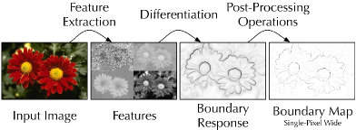
A canonical framework of boundary detection typically consists of three steps, i.e., feature extraction, differentiation and post-processing operations, as illustrated in Fig. 1. Taking mPb for an example, histograms of different cues and scales are firstly extracted. Then, the distance of descriptors from adjacent regions is calculated using $\chi^{2}$ difference. Finally, post-processing operations, such as noise reduction, cues fusion and oriented non-maximum suppression, are employed to generate single-pixel wide boundary maps as the output.

II-A Histogram-based Feature and $\chi^{2}$ Difference

In this letter, we adopt mPb [9] as the baseline and use exactly the same feature. Given a pixel $P(x,y)$ and the orientation $o\in[0,\pi)$, feature pairs of different cues and scales are extracted by pooling pixel-wise features over two half disks. As shown in Fig. 2, each pair of feature vectors, $U_{c,s}$ and $V_{c,s}$, corresponds to one kind of cue and a pooling scale. Both $U_{c,s}$ and $V_{c,s}$ are histograms which represent the distribution of cue $c$ within a half disk at scale $s$. Here 4 kinds of cues are considered, including 3 channels of Lab color space and 1 channel of textons. The number of pooling scales is also 4, indicating that 16 pairs of feature vectors are extracted at each pixel and each orientation.

Figure 2: Histogram-based feature of mPb. Given a pixel $P(x,y)$ and the orientation $o\in[0,\pi)$, a pair of features is extracted, denoted by $U_{c,s}$ and $V_{c,s}$. They are both histograms which represent the distribution of cue $c$ within a half disk at scale $s$. The value of $r_{s}$ depends on at which scale feature vectors are extracted. After feature extraction, $\chi^{2}$ difference is applied to calculate distance between $U_{c,s}$ and $V_{c,s}$.

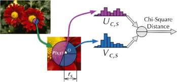
For the traditional approach of $\chi^{2}$ difference, each pair of feature vectors can be used to compute a distance $d_{c,s}$,

$$d_{c,s}=\frac{1}{2}\sum_{m}{\frac{(U_{c,s,m}-V_{c,s,m})^{2}}{U_{c,s,m}+V_{c,s,m}}}\;.$$ (1)

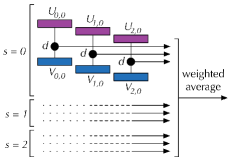
Then, all the distances computed in Eq. 1 are collected and summed up with respect to $c$ and $s$, weighted by $w_{c,s}$ obtained from logistic learning,

$$d=\sum_{c=0}^{3}{\sum_{s=0}^{3}{w_{c,s}d_{c,s}}}\;.$$ (2)

The result $d$ characterizes the boundary strength at pixel $P$ and orientation $o$. The pipeline of mPb is illustrated in Fig. 3(a).

The $\chi^{2}$ difference approach of mPb has a shortcoming in which supervising information affects only the weights $w_{c,s}$, while most parts of the algorithm are human-crafted. Restricted by the number of tunable parameters, the algorithm cannot fit the image data very well. In fact, if distances $d_{c,s}$ are summed up with equal weights, the F-measure metric on BSDS500 remains almost the same. Table I demonstrates the results of mPb with both learned weights and equal weights. ODS or OIS in the table refers to the best F-measure for the entire dataset or per image respectively, and AP (Average Precision) is the area under the PR curve. Details of evaluation method can be found in Section III.

TABLE I: Evaluation Results of mPb

	ODS	OIS	AP
mPb (with learned weights)	0.69	0.71	0.68
mPb (with equal weights)	0.69	0.71	0.70

II-B Learning Optimal Boundary Metric

According to the aforementioned analysis, the learning stage of mPb achieves limited improvements. To obtain better results, it is necessary to increase the number of tunable parameters. In this section, boundary metric is introduced, which is then optimized with respect to the loss function defined by Eq. 7.

As is known, Artificial Neural Network (ANN) is widely recognized for its strong fitting capability. Accordingly, the proposed LBM builds a neural network for each cue and scale to transform the local features into a new space. Then the distance of features is computed in the transformed space. In this manner, supervising information can be used to learn a better space where the metric is more consistent with human annotations. Assuming $f_{c,s}(\cdot)$ is the transformation corresponding to cue $c$ and scale $s$, the new distance can be formatted as follows,

$$d_{c,s}^{LBM}=D(\widetilde{U}_{c,s},\widetilde{V}_{c,s})=D(f_{c,s}(U_{c,s}),f_{c,s}(V_{c,s}))\;,$$ (3)

where $D(\cdot,\cdot)$ is the metric of the learned space. In this letter, we propose to use a group of logistic functions to implement the transformation,

$$\begin{split}\widetilde{U}_{n}&=f_{n}(U)=\frac{1}{1+e^{-\alpha_{n}-\sum_{m=1}^{M}{\beta_{n,m}U_{m}}}},\\ \widetilde{U}&=[\widetilde{U}_{1},\widetilde{U}_{2},\cdots,\widetilde{U}_{N}]^{T}\;.\end{split}$$ (4)

$M$ and $N$ in the formula denote the dimensions of input and output features, respectively. After the transformation, RBF kernel rather than linear kernel is adopted to compute the distance, because nonlinear kernel is more suitable for complex data such as natural images,

$$D(\widetilde{U},\widetilde{V})=1-e^{-\frac{\sum_{n=1}^{N}{(\tilde{U}_{n}-\tilde{V}_{n})^{2}}}{2\sigma^{2}}}\;.$$ (5)

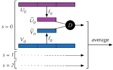
Until now, we have introduced the basic structure of LBM. In the final implementation, feature vectors of the same scale are concatenated to form a single vector, allowing more interactions among different cues. Then, a larger neural network is learned for $U_{s}=[U_{0,s}^{T},U_{1,s}^{T},U_{2,s}^{T},U_{3,s}^{T}]^{T}$. In the end, the mean of descriptor distances at all scales, $d^{LBM}$, is computed as output of the boundary response,

$$\begin{split}d_{s}^{LBM}&=D(\widetilde{U}_{s},\widetilde{V}_{s})=D(f_{s}(U_{s}),f_{s}(V_{s})),\\ d^{LBM}&=\frac{1}{4}\sum_{s=0}^{3}{d_{s}^{LBM}}\;.\end{split}$$ (6)

The pipeline of LBM is illustrated in Fig. 3(b) as a comparison with the mPb approach.

(a) $\chi^{2}$ difference approach

(b) LBM approach

Figure 3: Pipelines of (a) the baseline and (b) the proposed LBM method. In (a) distances are calculated between all pairs of feature vectors $U_{c,s}$ and $V_{c,s}$. The black nodes in the figure denote the $\chi^{2}$ difference. The final output is the weighted average of distances of all cues at all scales. In (b) the LBM method concatenates feature vectors of the same scale into a single vector $U_{s}$. Then the learning-based transformation $f_{s}$ is applied on $U_{s}$ and $V_{s}$. At each scale, metric $D$ based on RBF kernel, shown as the black node, is used to compute distances between the transformed features $\widetilde{U}_{s}$ and $\widetilde{V}_{s}$. The final output is the average of distances at all scales. The difference between the two approaches lies in the mechanism of metric design, either (a) human-crafted or (b) fine-tuned by supervised learning.

With the above definitions, the next step is to learn parameters $\alpha_{n}$ and $\beta_{n,m}$ according to human annotations. We define a loss function to indicate how well the neural networks fit the data, and then use Stochastic Gradient Descent (SGD) to tune the parameters. A simple way to define the loss function is directly using $d^{LBM}$, where losses of boundary and non-boundary pixels are $1-d^{LBM}$ and $d^{LBM}$ respectively. However, we prefer the log-style loss function since the gradient of a non-boundary pixel won’t be zero when $d^{LBM}=1$. In the following definition, $k$ denotes the index of training samples and $y_{k}$ is the annotation,

$$L=-\sum_{k=1}^{K}{y_{k}\log{d^{LBM}}+(1-y_{k})\log{(1-d^{LBM})}}\;.$$ (7)

$y_{k}=1$ indicates that the $k$th sample is a boundary pixel and vice versa.

To generate training samples, $\alpha_{n}$ and $\beta_{n,m}$ are randomly initialized, sampled uniformly from range $[-1,1]$. Then the algorithm selects a random image from the training set to detect boundary pixels with current parameters. The pixels matched to human annotations are collected as positive training set, while those without any match are regarded as the negative set. After that, SGD is performed to update the parameters. Next, another image is selected and the same process is repeated. We terminate the learning loop if the F-measure metric on validating set no longer has a noticeable improvement. In our implementation, boundary metrics at different scales are learned separately.

III Experiments

The proposed LBM is evaluated on BSDS500. The dataset contains 200 testing images, with about 5 annotations from different persons for each image. We follow the widely used evaluation measurement proposed by [10], in which a Precision-Recall (PR) curve is drawn and the F-measure metric is used for comparison.

A boundary pixel is counted as false alarm iff it does not match any annotation pixels. Note that it is common that several persons annotate the same pixel as ground truth, so the pixel may be counted as recall for several times. If the input boundary responses are real values rather than binary, a series of thresholds are utilized to obtain the PR curve.

There are 3 parameters which need to be determined before the learning stage. The first one is $N$, the dimension of the transformed feature space. The second one is $\sigma$ in the RBF kernel. With exhaustive search, we choose $N=16$ and $\sigma=0.2$, with which the algorithm achieves the best performance on validating set. The last parameter is learning rate. Large learning rate results in unstable SGD, while small learning rate leads to slow convergence. We set learning rate to 0.0001 as a trade off between robustness and learning efficiency. Other parameters, including $\alpha_{n}$ and $\beta_{n,m}$ in Eq. 4, are learned from human annotations. The evaluation results during the learning process indicate that the F-measure, as well as $\alpha_{n}$ and $\beta_{n,m}$ in Eq. 4, converges smoothly after dozens of iterations.

Although the structure of LBM is more complicated than that of $\chi^{2}$ difference, our algorithm requires much less computing resource. To extract $U_{c,s}$ or $V_{c,s}$ in Fig. 2, the original work needs to perform average pooling in a high dimensional feature space. However, dimension of $\widetilde{U}_{c,s}$ or $\widetilde{V}_{c,s}$ in LBM is very low, which means the pooling operation can be accelerated. Using the same computer with Intel i7-2600 and 16GB RAM to test both algorithms, LBM is able to achieve a $5\times$ speed-up.

Figure 4: Precision-recall curves on BSDS500 benchmark. (a) Comparison between $\chi^{2}$ difference and LBM using mPb features. After substituting $\chi^{2}$ difference with LBM, the F-measure metric of mPb is improved from 0.69 to 0.71. (b) Comparison between $\chi^{2}$ difference and single scale LBM. Even if only features at a single scale are available, LBM achieves competitive results compared with multi-scale approach of $\chi^{2}$ difference. (c) Comparison between $\chi^{2}$ difference and LBM, both with globalization. gPb is the globalized version of mPb, where an extra step of bootstrap is introduced. After applying the same globalization method, LBM also yields better results than gPb. All curves of LBM in this figure are results of LBM with RBF kernel.

Figure 5: Examples from the BSDS500 dataset. Top row is source image, middle row is gPb output, and bottom row is LBM output with globalization (this work). One advantage of our LBM approach is that some hard boundaries are enhanced, such as the mountain and windmill. Meanwhile, noisy boundaries of the red car, worm and owl are suppressed.

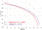
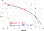
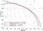
Extensive experiments are conducted to verify the effectiveness of LBM. Results are shown in Table II, Fig. 4 and Fig. 5. In Table II, ODS or OIS refers to the best F-measure for the entire dataset or per image respectively, and AP (Average Precision) is the area under the PR curve. Apart from original images, noisy condition is also considered. Here, we use Matlab R2012a to add Gaussian noise with default parameter. To show the effectiveness of RBF kernel, results of boundary metric using linear kernel are presented in Table II as well.

According to results of experiment 1 and 2, our algorithm compares favorably with the baseline approach, for both original images and noisy ones. After substituting $\chi^{2}$ difference with LBM, the F-measure metric of mPb is improved from 0.69 to 0.71. The major advantage of LBM consists in the increase of maximum recall, from 0.90 to 0.94 as shown in Fig. 4, indicating that about 40% of the missing pixels of baseline approach are detected by LBM. This results from the strong fitting capability of ANN, which captures all kinds of variations of natural image data. Experiment 3 only makes use of features at a single scale. We find that the single scale LBM achieves competitive performance compared with multi-scale approach of $\chi^{2}$ difference, as shown in Fig. 4. Compared with the original mPb, LBM learns more useful information from human annotations. The effectiveness of the learning stage of LBM can be confirmed by comparing the results in Table I and Table II.

TABLE II: Comparisons between $\chi^{2}$ Difference and LBM

Method		Original Image			Noisy Image
		ODS	OIS	AP	ODS	OIS	AP
1	mPb + $\chi^{2}$ difference	0.69	0.71	0.68	0.67	0.68	0.67
2	mPb + LBM (RBF)	0.71	0.74	0.73	0.69	0.71	0.72
3	Pb + LBM (RBF)	0.69	0.71	0.70	-	-	-
4	mPb + LBM (linear)	0.70	0.73	0.74	-	-	-
5	gPb + $\chi^{2}$ difference	0.71	0.73	0.73	0.69	0.70	0.70
6	gPb + LBM (RBF)	0.73	0.75	0.78	0.71	0.72	0.76
7	gPb + LBM (linear)	0.72	0.74	0.77	-	-	-

In [9], the authors introduce a globalization method as a bootstrap to further improve the performance of mPb. The new algorithm is named as gPb. The proposed LBM can also be integrated into the framework of gPb. In the original work, boundary responses computed by the bootstrap step is multiplied by a learned weight and added to mPb output. We follow a similar strategy, using the algorithm introduced by [14] to learn the weight. According to experiment 5 and 6, all 3 measurements of LBM produce better results than gPb. Corresponding PR curves can be found in Fig. 4. Apart from PR curves, standard deviation of best F-measures for each image is also computed to show the statistical significance of the improvement. The standard deviation of $gPb$ + LBM (RBF) is $9.75\times 10^{-3}$, while that of $gPb$ + $\chi^{2}$ difference is $9.83\times 10^{-3}$. In addition, LBM obtains superior results in 131 out of 200 testing images. Fig. 5 shows some examples. One advantage of our LBM approach is that some hard boundaries are enhanced, such as the mountain and windmill. Meanwhile, noisy boundaries of the red car, worm and owl are suppressed. What is more, these results are competitive with the state-of-the-art results reported in [15] (ODS: 0.74, OIS: 0.76 and AP: 0.77), which take advantage of sparse coding based local features.

IV Conclusion

In this letter, a Learning-based Boundary Metric (LBM) is proposed to substitute the $\chi^{2}$ difference used in mPb. One of the advantages of LBM is the strong fitting capability of natural image data. With supervised learning, LBM is able to learn useful information from human annotations, while the learning stage of mPb achieves only limited improvements. The structure of LBM is easy to understand, composed of a single layer neural network and an RBF kernel. With the above advantages, LBM yields better performance than both mPb and gPb. Extensive experiments are conducted to verify the effectiveness of LBM. The F-measure metric on BSDS500 benchmark is increased to 0.71 (without globalization) and 0.73 (with globalization) respectively. In the future, we are interested in applying LBM to the framework of SCG, which achieves the state-of-the-art performance.

References

- [1] A. Opelt, A. Pinz, and A. Zisserman, “A boundary-fragment-model for object detection,” in ECCV, 2006, pp. 575–588.
- [2] J. Shotton, A. Blake, and R. Cipolla, “Multiscale categorical object recognition using contour fragments,” IEEE Trans. Pattern Analysis and Machine Intelligence, vol. 30, no. 7, pp. 1270–1281, 2008.
- [3] A. Farhadi, I. Endres, D. Hoiem, and D. Forsyth, “Describing objects by their attributes,” in CVPR, 2009, pp. 1778–1785.
- [4] V. Ferrari, F. Jurie, and C. Schmid, “From images to shape models for object detection,” Int’l J. of Computer Vision, vol. 87, no. 3, pp. 284–303, 2010.
- [5] J. Canny, “A computational approach to edge detection,” IEEE Trans. Pattern Analysis and Machine Intelligence, vol. 8, no. 6, pp. 679–698, 1986.
- [6] P. Dollar, Z. Tu, and S. Belongie, “Supervised learning of edges and object boundaries,” in CVPR, 2006, pp. 1964–1971.
- [7] I. Kokkinos, “Boundary detection using f-measure-, filter- and feature- (f3) boost,” in ECCV, 2010, pp. 650–663.
- [8] R. Kennedy, J. Gallier, and J. Shi, “Contour cut: Identifying salient contours in images by solving a hermitian eigenvalue problem,” in CVPR, 2011, pp. 2065–2072.
- [9] P. Arbelaez, M. Maire, C. Fowlkes, and J. Malik, “Contour detection and hierarchical image segmentation,” IEEE Trans. Pattern Analysis and Machine Intelligence, vol. 33, no. 5, pp. 898–916, 2011.
- [10] D. Martin, C. Fowlkes, and J. Malik, “Learning to detect natural image boundaries using local brightness, color, and texture cues,” IEEE Trans. Pattern Analysis and Machine Intelligence, vol. 26, no. 5, pp. 530–549, 2004.
- [11] X. Ren, “Multi-scale improves boundary detection in natural images,” in ECCV, 2008, pp. 533–545.
- [12] D. Martin, C. Fowlkes, D. Tal, and J. Malik, “A database of human segmented natural images and its application to evaluating segmentation algorithms and measuring ecological statistics,” in ICCV, 2001, pp. 416–423 vol.2.
- [13] E. P. Xing, A. Y. Ng, M. I. Jordan, and S. Russell, “Distance metric learning with application to clustering with side-information,” in NIPS, 2003, pp. 505–512.
- [14] M. Jansche, “Maximum expected f-measure training of logistic regression models,” in Proceedings of the Conference on Human Language Technology and Empirical Methods in Natural Language Processing, 2005, pp. 692–699.
- [15] X. Ren and L. Bo, “Discriminatively trained sparse code gradients for contour detection,” in NIPS, 2012, pp. 593–601.