Systematic Law for Half-lives of Double $\beta$-decay with Two Neutrinos

Abstract

Nuclear double $\beta$-decay with two neutrinos is a rare and important process for natural radioactivity of unstable nuclei. The experimental data of nuclear double $\beta^{-}$-decay with two neutrinos are analyzed and a systematic law to calculate the half-lives of this rare process is proposed. It is the first analytical and simple formula for double $\beta$-decay half-lives where the leading effect from both the Coulomb potential and nuclear structure is included. The systematic law shows that the logarithms of the half-lives are inversely proportional to the decay energies for the ground state transitions between parent nuclei and daughter nuclei. The calculated half-lives are in agreement with the experimental data of all known eleven nuclei with an average factor of 3.06. The half-lives of other possible double $\beta$-decay candidates with two neutrinos are predicted and these can be useful for future experiments. The law, without introducing any extra adjustment, is also generalized to the calculations of double $\beta$-decay half-lives from the ground states of parent nuclei to the first $0^{+}$ excited states of daughter nuclei and the calculated half-lives agree very well with the available data. Some calculated half-lives are the first theoretical results of double $\beta$-decay half-lives from the ground states of parent nuclei to the first $0^{+}$ excited states of daughter nuclei. The similarity and difference between the law of $\alpha$-decay and that of double $\beta^{-}$-decay are also analyzed and discussed.

The discovery of natural radioactivity by Becquerel changed our views on the structure of matters and promoted the development of modern physics and modern chemistry. Rutherford identified that there are three kinds of natural radioactivity and named them as $\alpha$-, $\beta$- and $\gamma$-rays li1 ; pre ; sha ; wa1 . The structure of an atom is clear when Rutherford proposed the existence of a nucleus in an atom based on $\alpha$-scattering experiments with $\alpha$-particles from natural radioactivity. Researches on the problem of energy conservation in a $\beta$-decay process lead to Pauli’s suggestion of the existence of a new particle, neutrino. Based on this idea, Fermi proposed the basic formulation of the weak interaction for the description of $\beta$-decay of a nucleus. In 1956, Lee and Yang proposed that parity cannot conserve for a weak process such as $\beta$-decay lee . Wu and her collaborators carried out the $\beta$-decay experiment with polarized ${}^{60}Co$ nuclei and observed that parity symmetry was broken wu . The vector and axial-vector theory (V-A) of the weak interaction for four fermions was founded in 1958 fey ; sud and is still widely used for the calculations of $\beta$-decay half-lives and double $\beta$-decay half-lives hax ; eji ; Int . The unification of weak and electromagnetic interactions is reached with the discovery of intermediate bosons and the standard model is well founded with the experimental confirmation of the Higgs particle. Currently new progress on physics processes with neutrinos or without neutrinos is being made. Some important processes with neutrinos are the measurement of $\theta_{13}$ in neutrino oscillations and the weak processes such as the neutrino-induced reaction and the double $\beta$-decay with neutrinos. An important process without neutrinos is the search of the nuclear double beta decay without emission of neutrinos. In this article we focus on the research of half-lives of double $\beta$-decay with two neutrinos.

There are many experimental and theoretical researches on double $\beta$-decay with two neutrinos and without neutrinos hax ; eji ; ack ; gan ; arn ; bar ; saa ; aud1 ; aud2 ; kla ; rad ; avi ; ago ; fae1 ; fae2 ; cau ; suh ; suo ; vog ; ver . A list of available experimental data on decay energies and half-lives can be found in recent review articles bar ; saa and in nuclear data tables aud1 ; aud2 . Some recent experimental results on the half-lives of ${}^{130}Te$ are published in reference arn and those of ${}^{136}Xe$ are published in references ack ; gan . Very recent data of ${}^{76}Ge$ are reported in reference ago . As experimental data are accumulated for 11 double $\beta$-decay nuclei with neutrinos, to make a systematic analysis on them and to find a systematic law of data are useful for future researches.

Theoretically there are two kinds of calculations on double $\beta$-decay half-lives and nuclear matrix elements hax ; fae1 ; avi . One is based on the nuclear shell model with an effective interaction from a renormalized g-matrix obtained with the Bonn potential hax ; fae1 ; avi ; cau . Another is based on the quasi-particle random-phase approximation (QRPA) or self-consistent renormalized random-phase approximation (RQRPA) hax ; fae1 ; avi where the collective particle-hole excitation of nuclei is included and the intermediate-nucleus states are represented as a set of phonon states hax ; fae1 ; avi . A recent review can be found in reference avi . These calculations are very successful for the description of the double $\beta$-decay half-lives and nuclear matrix elements due to the much effort of theoretical physicists. They are in general very complicated, and require both sophisticated computer codes and experiences in the specific problem to generate results which can be compared with those obtained in the laboratory. And in many cases different models generate different predictions, which can be no easily reconciled. In the cases of the two neutrino double $\beta$-decay, after decades of research there are plenty of theoretical half-lives for many possible candidates based on the calculations with the nuclear shell model or with the various quasi-particle random-phase approximation. Although plenty of theoretical half-lives were reported for many nuclei, some recent experimental data are not covered by the calculations saa . For example, it is observed there is the double $\beta$-decay from the ground state of ${}^{150}Nd$ to the first excited $0^{+}$ state of its daughter nucleus and there is no theoretical half-life on this saa . Therefore further calculation on double $\beta$-decay half-lives is needed. Because there are plenty of calculations based on the the nuclear shell model and the various quasi-particle random-phase approximation, we do not carry out similar calculations to them and we try a different way to investigate the double $\beta$-decay half-lives in this article. It is believed that the different approach to double $\beta$-decay is useful for future development of the field and is also useful for future experimental research. It is widely accepted that only experimental data themselves can test the reliability of the prediction of the different approaches in physics.

At first we make a systematic analysis on the available data of double $\beta$-decay to the ground state of daughter nuclei. Up to now there are 11 nuclei which are observed to have double $\beta$-decay with two neutrinos and their decay energies and half-lives are listed in Table 1. In Table 1, the first column denotes the parent nucleus and the second column represents the experimental double $\beta$-decay half-life for the ground-state transition between the parent nucleus and the daughter nucleus. The experimental double $\beta$-decay half-lives are mainly presented in the references bar ; saa ; aud1 and here the data are from reference saa . We also list the logarithm of the half-life in column 3. Column 4 is the experimental double $\beta$-decay energy of the nucleus from the ground state of the parent nucleus to the ground state of daughter nucleus where the data are from the nuclear mass table by Audi et al. and Wang et al. aud1 ; aud2 . The units of half-lives are Ey ($10^{18}$ years). The fifth column represents the square root of the multiplication between the logarithm of experimental half-life and the decay energy.

Table 1: The experimental data of double $\beta$-decay half-lives (T${}_{1/2}(expt.)$) and decay energies ($Q_{2\beta}$) of 11 even-even nuclei. In order to analyze the law of the data we also list the logarithm of double $\beta$-decay half-lives and the square root of the multiplication between the logarithm of experimental half-life and the decay energy in columns 3 and 5, respectively. The units of the half-lives are Ey ($10^{18}$ years). The experimental half-lives and decay energies in the table are from references saa and aud2 , respectively.

Nuclei	T${}_{1/2}(expt.)$(Ey)	lgT${}_{1/2}(expt.)$	$Q_{2\beta}$(MeV)	$\sqrt{lgT_{1/2}(expt.)}\,\sqrt{Q_{2\beta}(expt.)}$)
48Ca	$44^{+6}_{-5}$	1.643	4.267	2.649
76Ge	$1840^{+140}_{-100}$	3.265	2.039	2.580
82Se	$92^{+7}_{-7}$	1.964	2.996	2.424
96Zr	$23.5\pm{0.21}$	1.371	3.349	2.143
100Mo	$7.1\pm{0.4}$	0.851	3.034	1.606
116Cd	$28\pm{2}$	1.447	2.813	2.017
128Te	$(1.9\pm{0.4})\times 10^{6}$	6.279	0.8665	2.333
130Te	$700\pm{140}$	2.845	2.528	2.682
136Xe	$2300\pm{120}$	3.362	2.458	2.876
150Nd	$9.11\pm{0.68}$	0.960	3.371	1.799
238U	$2000\pm{600}$	3.301	1.144	1.944

It is seen from Table 1 that the shortest half-life is $7.1\ Ey$ for ${}^{100}Mo$ and the longest is $1.9\times 10^{6}\ Ey$ for ${}^{128}Te$. The half-lives vary from $7.1\ Ey$ (${}^{100}Mo$ ) to $1.9\times 10^{6}\ Ey$ (${}^{128}Te$) although the change of the decay energies is less than four times ( from 3.034 MeV for ${}^{100}Mo$ to 0.8665 MeV for ${}^{128}Te$). This shows that the half-life is very sensitive to the decay energy and the relationship between them may be very complex by a glance of the data. In order to describe quantitatively the sensitivity and to find a law among the data, we introduce the logarithm of the half-life and also make a square root for the multiplication between the logarithm of the half-life and the decay energy. The square root of the multiplication is listed in the last column of Table 1. It is clearly seen from the last column that the variation of the square root of the multiplication is in a very narrow range from the minimum 1.606 to the maximum 2.876. This fact strongly suggests that a constant value can be a good approximation for the multiplication of the logarithm of the half-lives and decay energies. The physics behind this will be discussed later in this article. This is the starting point of our researches and we simply write it in the following mathematical equation between the logarithm of half-life and the decay energy,

$$lg\,T_{1/2}(Ey)\,=\,a\,/{Q_{2\beta}(MeV)}$$ (1)

Here $a$ is a constant and its value is to be determined. We will discuss the meaning of this constant later and will point out that the constant $a$ is from the universal properties of the weak interaction for the decay process of different nuclei.

For a better description of the double $\beta$-decay half-lives, the effects from the Coulomb potential and from nuclear structure should be taken into account. It is well known from the $\beta$-decay theory pre ; sha ; wa1 that the effect from the Coulomb potential can be derived from quantum mechanics and its expression in the nonrelativistic case is given in some textbooks pre ; sha ; wa1 ,

$$\rho(Z,\epsilon)\,=\,2\,\pi\eta/(1-e^{-2\,\pi\eta})$$ (2)

where $\eta=\,(Z/137)\,(\epsilon/cp)$ and $\epsilon$ is the energy of electron and $p$ is the magnitude of the electron momentum.

Usually the correction of the Coulomb potential should multiply the square of the matrix element to obtain the probability of $\beta$-decay pre ; sha ; wa1 . This correction factor is close to unity for light nuclei but it has an evident effect for heavy nuclei. In the usual $\beta$ decay or the double $\beta$-decay of this article, the speed of an electron is very close to the speed of light ($v_{e}\approx 0.86-0.95\,c$) and therefore $(\epsilon/cp)$ is close to unity. For the denominator of Eq.(2) it is also a good approximation to choose it to be unity for heavy nuclei. Therefore we only keep the leading term of equation (2) for simplicity and a correction of the Coulomb potential for double $\beta$-decay half-lives is approximately $-2\,lg((2\pi Z)/137)$ to the numerator of equation (1) where Z is chosen to be the charge number of parent nuclei and this is also for the convenience of calculations. This correction is approximately zero for light double $\beta$-decay nuclei such as ${}^{48}Ca$ and it can give significant contribution for heavy nuclei such as ${}^{238}U$.

Now let us take the nuclear structure effect into account to some extent. We keep with the same spirit to the correction of the Coulomb potential and only include the leading effect from the strong interaction. For nuclear structure, the most important effect from the strong interaction of nucleons is the existence of magic numbers and this corresponds to the appearance of nuclear shell structure in nuclei. The nuclei with magic number are more stable than non-magic nuclei. For the numerical calculations of both shell model and mean-field model, the first step is the choice of the number of valence nucleons. The choice of the number of valence nucleons is with reference to magic numbers. The number of valence neutrons of a nucleus is zero if its neutron number corresponds to a magic number. The valence neutron number of a nucleus is not zero if its neutron number does not correspond to a magic number. The parameters of the effective mean-field potential in a self-consistent mean-field model are often obtained with the fitting of ground state properties of several magic nuclei such as ${}^{16}O$, ${}^{40,48}Ca$, and ${}^{208}Pb$ and the residual interaction such as the pairing force is included for valence nucleons when it is used for researches of open shell nuclei. For the double $\beta$-decay process it involves a change of two neutrons into two protons for nuclei with the same nucleon number (A). It can be observed if other decay mode such as a single $\beta$-decay is forbidden in energy. Based on this we simulate the leading effect of nuclear structure (i.e. shell effect) by introducing an addition quantity $S$ to the numerator of equation (1). $S=2$ when the neutron number of a parent nucleus is a magic number and $S=0$ when the neutron number is non-magic. Whether this choice is suitable can be tested by the numerical results of this article. In this way we do not touch the details of the complex nuclear potential and we also avoid solving the very complicated nuclear many-body problem. So a new systematic law of double $\beta$-decay half-lives is proposed to be

$$lg\,T_{1/2}(Ey)\,=\,(a\,-2\,lg(2\,\pi\,Z/137)\,+\,S\,)\,/\,{Q_{2\beta}(MeV)}$$ (3)

where the constant $a$ is obtained by fitting the experimental data of Table 1 and its value is $a=5.843$. We will point out later that the physical meaning of $a$ is related to the square of the strength of the weak interaction which leads to the instability of a nucleus. $Z$ is the charge number of the parent nucleus. $S=2$ when the neutron number of parent nuclei is a magic number and  $S=0$ when the neutron number of parent nuclei is not a magic number. The number of parameters of equation (3) is two if both $a$ and $S$ are considered to be adjusting parameters. The number of parameters of equation (3) is one if only $a$ is considered to be an adjusting parameter and if $S$ is accepted to be from the shell effect (in the shell model and in the mean-field model people naturally choose the valence number with reference of magic numbers). In a word, the number of adjusting parameters in equation (3) is the least as compared to a model with an effective potential because one needs two parameters (depth and force range) to define a central potential and a third parameter to define the strength of the spin-orbit potential. Because the equation (3) is very clear and simple, any physicists including experimental physicists can use it to calculate the half-lives of double $\beta$-decay with inputs of the decay energies. A pocket calculator with logarithm function is enough to get numerical results.

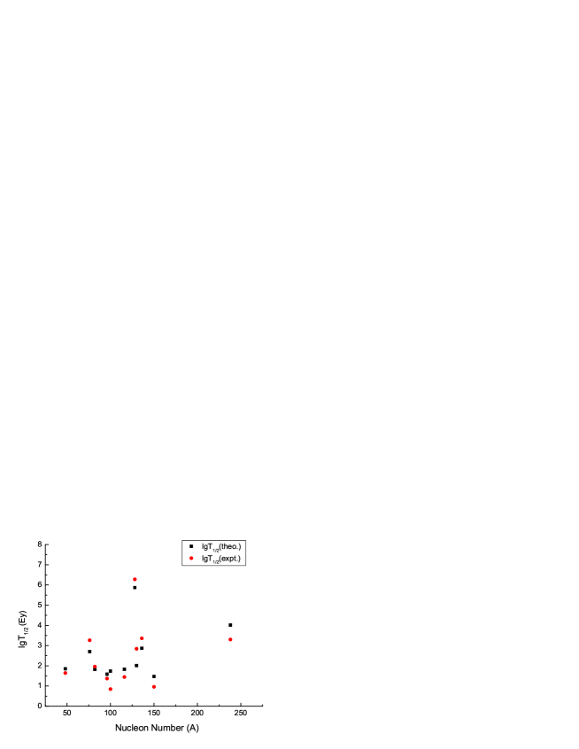
Figure 1: Logarithms of the experimental double $\beta$-decay half-lives and theoretical ones for ground-state transitions of 11 even-even nuclei from ⁴⁸Ca to ²³⁸U. The calculated half-lives are in agreement with the experimental data of all known eleven nuclei with an average factor of 3.06. The maximum deviation between theoretical half-life and experimental one is a factor of 7.709 and this corresponds to the case of ${}^{100}Mo$.

The numerical results from equation (3) are drawn in Figure 1 and also listed in Table 2, together with experimental half-lives and decay energies. In Fig.1, the X-axis is the nucleon number and the Y-axis is the logarithm of the double $\beta$-decay half-lives. Experimental data and calculated results with equation (3) are denoted with different symbols in the figure. It is seen that the calculated results are close to experimental data and reasonable agreement is achieved for eleven nuclei which are observed to have double $\beta$-decay with two neutrinos. We make a detailed discussion on the calculated results of Table 2. In Table 2 columns 1-4 are experimental data and they have the same meaning as columns 1-4 of Table 1. Column 5 is the logarithm of the calculated double $\beta$-decay half-lives with equation (3). The last column is the logarithm of the ratio between experimental double $\beta$-decay half-lives and calculated ones and it shows the deviation between experimental half-lives and calculated ones. When the deviation is less than 0.301, the agreement between the experimental half-life and the calculated one is within a factor of two (lg2=0.301) and this corresponds to the cases for ${}^{48}Ca$, ${}^{82}Se$, ${}^{96}Zr$ . When the deviation is less than 0.477, the agreement between the experimental half-life and the calculated one is within a factor of three (lg3=0.477) and this is the case for ${}^{116}Cd$ and ${}^{128}Te$. It is seen from Table 2 that experimental half-lives can be reproduced by calculations within a factor of four for eight nuclei (lg4=0.602) (such as the case of ${}^{76}Ge$, ${}^{136}Xe$ and ${}^{150}Nd$). The deviation between experimental half-lives and the calculated results is beyond a factor of four for three nuclei ${}^{100}Mo$,${}^{130}Te$, and ${}^{238}U$. For ${}^{238}U$ the agreement for half-lives is approximately a factor of 5.2 (lg5.2=0.716). For ${}^{100}Mo$ the calculation can reproduce its experimental half-life within a factor of eight (lg8=0.903) and for ${}^{130}Te$ the calculation can reproduce that within a factor of seven (lg7=0.845). In order to see the total agreement for eleven nuclei we define an average deviation $\Delta=\{\Sigma_{i=1}^{i=11}\ \left|lg(T_{1/2}(expt.)/T_{1/2}(theo.))\right|\}/11=0.486$. This corresponds to a factor of 3.06 between experimental half-lives and calculated ones (lg3.06=0.486). This agreement between double $\beta$-decay half-lives and calculations with equation (3) is good compared with the calculations of single $\beta$-decay half-lives ni6 ; ni7 ; li6 ; zha ; mol and ${\alpha}$-decay half-lives of unstable nuclei ni1 ; ni2 ; ren ; ren3 . Especially the calculations of this article are with the minimum number of adjusting parameters and cover a wide range of nuclear mass from $A=48$ (${}^{48}Ca$) to $A=238$ (${}^{238}U$). This means it can be used to predict the double $\beta$-decay half-lives of other nuclei in nuclide charts.

Table 2: The logarithm of double $\beta$-decay half-lives of even-even isotopes calculated with new law ($lgT_{theo.}$) and the corresponding experimental ones ($lgT_{expt.}$). The units of the half-lives are Ey ($10^{18}$ years). The experimental decay energies of nuclei ($Q_{2\beta}$ (MeV)) are also listed in the table where the decay energies are from the nuclear mass table aud2 . The calculated half-lives are in agreement with the experimental data of all known eleven nuclei with an average factor of 3.06. The maximum deviation between theoretical half-life and experimental one is a factor of 7.709 and this corresponds to the case of ${}^{100}Mo$.

Nuclei	T${}_{1/2}(expt.)$(Ey)	$lgT_{1/2}(expt.)$	$Q_{2\beta}$(MeV)	$lgT_{1/2}(theo.)$	$lg(T_{1/2}(expt.)/T_{1/2}(theo.))$
48Ca	$44^{+6}_{-5}$	1.643	4.267	1.856	-0.213
76Ge	$1840^{+140}_{-100}$	3.265	2.039	2.702	+0.563
82Se	$92^{+7}_{-7}$	1.964	2.996	1.822	+0.142
96Zr	$23.5\pm{0.21}$	1.371	3.349	1.587	-0.216
100Mo	$7.1\pm{0.4}$	0.851	3.034	1.738	-0.887
116Cd	$28\pm{2}$	1.447	2.813	1.834	-0.378
128Te	$(1.9\pm{0.4})\times 10^{6}$	6.279	0.8665	5.872	0.407
130Te	$700\pm{140}$	2.845	2.528	2.013	0.832
136Xe	$2300\pm{120}$	3.362	2.458	2.871	0.491
150Nd	$9.11\pm{0.68}$	0.960	3.371	1.473	-0.513
238U	$2000\pm{600}$	3.301	1.144	4.015	-0.714

In Table 3 we predict the double $\beta$-decay half-lives with two neutrinos for eleven nuclei. This corresponds to the decays between the ground states of parent nuclei and daughter nuclei and their mass numbers lie in a very wide range from ${}^{46}Ca$ to ${}^{244}Pu$. They are the good candidates to observe the double $\beta$-decay with two neutrinos. In Table 3, the first column denotes the parent nuclei and the second column is the experimental decay energies where the experimental data are from the nuclear mass tables aud1 ; aud2 . The third column corresponds to the logarithm of calculated half-lives with equation (3). We also list the double $\beta$-decay half-lives in the last column and this is convenient to make a direct comparison with future double $\beta$-decay experiments. The decay energies of these nuclei vary approximately from 1 MeV to 2 MeV and their half-lives range approximately from $10^{2}$ Ey to $10^{6}$ Ey. These will be tested by future measurements.

Recently it is also observed that the double $\beta$-decay with two neutrinos can occur from the ground state of parent nuclei to the first $0^{+}$ excited state of daughter nuclei saa . Based on the successful description of the double $\beta$-decay half-lives of ground-state transitions with equation (3), we now generalize the equation (3) to the calculation of double $\beta$-decay half-lives to the first $0^{+}$ excited state of daughter nuclei. We list the numerical results in Table 4, together with experimental decay energies and two experimental half-lives from the decay of ${}^{100}Mo$ and ${}^{150}Nd$ to the first $0^{+}$ excited state of the daughter nuclei saa . For the half-life from ${}^{100}Mo$, the calculated result is approximately the same as the experimental one. For that of ${}^{150}Nd$, the calculated result agrees with experimental one within a factor of two ($lg2=0.301$). It is seen without introducing any extra adjustment in the law that very perfect agreement is reached for the available data when the law is extended to the decay to the first $0^{+}$ excited state of daughter nuclei. This confirms the validity of the law. According to the newest review article of the double $\beta$-decay with two neutrinos saa , no theoretical half-life is reported for the decay from ${}^{150}Nd$ to the first $0^{+}$ excited state of the daughter nucleus. Therefore the calculated half-life of ${}^{150}Nd$ in Table 4 is the first theoretical result. Besides the experimental half-lives of ${}^{100}Mo$ and ${}^{150}Nd$, there are not definite half-lives from the measurement of other nuclei in Table 4 saa . Our calculated results are above the low limit of the half-lives for other nuclei saa .

Table 3: The double $\beta$-decay half-lives ($T_{1/2}(theo.)$) of even-even isotopes calculated with new systematic law and the corresponding logarithms ($lgT_{1/2}(theo.)$). The units of the half-lives are Ey ($10^{18}$ years). The experimental decay energies of nuclei ($Q_{2\beta}$ (MeV)) are also listed in the table where the decay energies are from the nuclear mass table aud2 .

Nuclei	$Q_{2\beta}$(MeV)	$lgT_{1/2}(theo.)$	$T_{1/2}(theo.)$(Ey)
46Ca	0.989	5.984	$9.64\times 10^{5}$
86Kr	1.258	5.889	$7.74\times 10^{5}$
94Zr	1.142	4.655	$4.52\times 10^{4}$
104Ru	1.301	4.023	$1.05\times 10^{4}$
110Pd	2.017	2.576	$3.77\times 10^{2}$
148Nd	1.928	2.575	$3.76\times 10^{2}$
154Sm	1.251	3.945	$8.81\times 10^{3}$
160Gd	1.731	2.835	$6.84\times 10^{2}$
198Pt	1.049	4.515	$3.27\times 10^{4}$
124Sn	2.291	2.236	$1.72\times 10^{2}$
244Pu	1.35	3.388	$2.44\times 10^{3}$

Table 4: This table corresponds to double $\beta$-decay from the ground state of parent nuclei to the first $0^{+}$ excited state of daughter nuclei (denoted with a symbol $*$). Column 1 represents the parent nuclei and column 2 denotes the experimental double $\beta$-decay half-lives saa . Our calculated half-lives from the systematic law are listed in column 4. The units of the calculated half-lives in column 4 are Ey ($10^{18}$ years). The experimental decay energies of nuclei ($Q^{*}_{2\beta}$ (MeV)) are also listed in the table where the experimental data are from reference saa . The calculated results of ⁴⁸Ca and ¹⁵⁰Nd are the first theoretical results according to Table 3 of the newest review article saa . The calculated results (Ey) from other groups are also listed in the last two columns for comparison and these are also taken from Table 3 of the review article saa .

Nuclei	$T^{*}_{1/2}(expt.)$(Ey)	$Q^{*}_{2\beta}$(MeV)	$T^{*}_{1/2}(theo.)$(Ey)	$T^{*}_{1/2}(other1.)$(Ey)	$T^{*}_{1/2}(other2.)$(Ey)
48Ca		1.275	$1.63\times 10^{6}$
76Ge		0.917	$1.02\times 10^{6}$	$(7.5-310)\times 10^{3}$ s41 ; s66	$4.5\times 10^{3}$ s67
82Se		1.506	$4.21\times 10^{3}$	$(1.5-3.3)\times 10^{3}$ s41 ; s66
96Zr		2.203	$2.59\times 10^{2}$	$(24-27)\times 10^{2}$ s41 ; s66	$38\times 10^{2}$ s67
100Mo	$5.9^{+0.8}_{-0.6}\times 10^{2}$	1.904	$5.89\times 10^{2}$	$16\times 10^{2}$ s74	$21\times 10^{2}$ s67
116Cd		1.048	$8.36\times 10^{4}$	$1.1\times 10^{4}$ s41 ; s66	$0.11\times 10^{4}$ s67
130Te		0.735	$8.38\times 10^{6}$	$(5.1-14)\times 10^{4}$ s41 ; s66 ; s76
150Nd	$1.33^{+0.45}_{-0.26}\times 10^{2}$	2.627	$0.776\times 10^{2}$

After we present numerical results for double $\beta$-decays to both the ground state and to the first $0^{+}$ excited state of daughter nuclei, it is useful to discuss the physics behind the new law. For this purpose we compare the differences and common points between $\alpha$-decay and double $\beta$-decay because both of them are two important decay modes of unstable nuclei. It is known that the half-lives of $\alpha$-decay can be calculated by the Geiger-Nuttall law or the Viola-Seaborg formula with a few parameters ni1 ; ren ; ren3 . A new version of the Geiger-Nuttall law is proposed ren and it can well reproduce the experimental half-lives of both $\alpha$-decay and cluster radioactivity ni1 ; ren ; ren3 . The new Geiger-Nuttall law between $\alpha$-decay half-lives (in seconds) and $\alpha$-decay energies (in MeV) of ground-state transitions of even-even nuclei is ren

$$lgT^{\alpha}_{1/2}(seconds)\,=\,a\,{\sqrt{\mu}}\,{Z_{c}}{Z_{d}}/{\sqrt{Q^{\alpha}}}+\,b{\sqrt{\mu}}{\sqrt{Z_{c}Z_{d}}}+\,c\,+\,S\,$$ (4)

In this equation the values of three parameters are $a=0.39961,b=-1.31008,c_{e-e}=-17.00698$ for even-even (e-e) nuclei ren . $T^{\alpha}_{1/2}$(seconds) is the half-life of $\alpha$-decay and $Q^{\alpha}(MeV)$ is the corresponding decay energy. $Z_{c}$ and $Z_{d}$ are the charge numbers of the cluster and the daughter nucleus, respectively. $\mu=A_{c}\,A_{d}/(A_{c}+A_{d})$ is the reduced mass and $A_{c}$,$A_{d}$ are the mass numbers of the cluster and daughter nucleus, respectively. For $\alpha$-decay, $Z_{c}$=2 and $A_{c}$=4. The three parameters, $a,b,c$, are obtained by fitting the data of even-even nuclei with $Z\geq 84$ and $N\geq 128$ ni1 . $S$ is a new quantum number to mock up the shell effect of N=126 on $\alpha$-decay half-lives. The value of $S$ for ground-state transitions of even-even nuclei is: $S=0$ for $N\geq\,128$ and $S=1$ for $\ N\leq\,126$ ren .

When we compare the new Geiger-Nuttall law of $\alpha$-decay half-lives (equation (4)) with the new systematic law of double $\beta$-decay half-lives (equation (3)), we find they are very similar although they are governed by different interactions. For a clear comparison, one can keep the first term of both laws temporarily because it is the leading term and the last two terms are the corrections to the leading term ( the constant $c$ in new Geiger-Nuttall law can be approximately eliminated if we change the units of the half-life from seconds to $10^{17}$ seconds). A common point between $\alpha$-decay and double $\beta$-decay is that their half-lives are very sensitive to the decay energy and the equations on their half-lives look alike. The first term in new Geiger-Nuttall law (equation (4)) is dependent on both charge numbers and decay energies because the Coulomb repulsive potential leads to the appearance of $\alpha$-decay (a quantum tunneling effect) and the total effect from the Coulomb potential is related to the charge numbers (similarly the total effect of the strong interaction is also directly related to the nucleon number of a nucleus). For the systematic law of double $\beta$-decay half-lives (equation (3)), the first term is only dependent on the decay energy because the weak interaction is universal for natural decay processes and the total effect from the weak interaction is not very sensitive to the change of nucleon numbers (such as proton numbers). This agrees with our knowledge of the weak interaction that the strength of the weak interaction of a free-neutron $\beta$-decay is approximately same as that of a $\mu$ decay although two decay systems are very different and the difference of their decay energies is approximately 100 times (of course the strength of a weak interaction can be different if different generation of quarks or different generation of leptons in Standard Models are involved.) It is due to the difference of this total effect between the weak interaction and the Coulomb interaction that $\beta$-decay occurs for the ground state of many unstable nuclei from very light ones (such as a decay from a neutron or from a triton) to heavy ones and $\alpha$-decay occurs for ground states of medium and heavy nuclei. Another important difference between the new systematic law and the Geiger-Nuttall law is from the difference of the perturbation approximation in quantum mechanics. The double $\beta$-decay is a second-order process of the weak interaction with the V-A four-fermion theory where a single $\beta$-decay is forbidden in many double $\beta$-decay nuclei. For the Geiger-Nuttall law, the $\alpha$-decay is a first-order process of the electromagnetic interaction and there are significant influences from the strong interaction. Before ending the discussion, we would like to point out that the right side of Eq.(3) can be dimensionless if one would like to replace the decay energy $Q_{2\beta}$ by $Q_{2\beta}/(2m_{e}c^{2})$. In this case the accuracy of calculated half-lives with the systematic law is almost kept due to $2m_{e}c^{2}=1.022\,MeV\,\approx 1\,MeV$.

In summary, the new law for the calculations of double $\beta$-decay half-lives is proposed where the leading effects of the decay energy, the Coulomb potential and the nuclear structure are naturally taken into account. This is the first analytical formula for the half-lives of the complex double $\beta$-decay with two neutrinos where only two parameters are used in the formula. By including these leading effects, the available data of double $\beta$-decay half-lives of ground-state transitions in even-even nuclei are reasonably reproduced. Without introducing extra adjustment on the two parameters of the law, the law is generalized to the double $\beta$-decay between the ground state of parent nuclei and the first $0^{+}$ excited state of daughter nuclei and perfect agreement between the calculated half-lives and the data is reached. The existence of these terms is based on the quantum theory for the microscopic description of the double $\beta$-decay process. The universal behavior of the weak interaction manifests itself in the formula of double $\beta$-decay half-lives by comparing the similarity and difference between the systematic law of double $\beta$-decay half-lives and the famous Geiger-Nuttall law of $\alpha$-decay. The half-lives of the double $\beta$-decay candidates with two neutrinos are predicted and they are useful for future experiments.

This work is supported by National Natural Science Foundation of China (Grant Nos. 11035001, 10975072, 11120101005, 11175085), by the Research Fund of Doctoral Point (RFDP), No. 20070284016 and by the Priority Academic Program Development of Jiangsu Higher Education Institutions.

References

- (1) J. S. Lilley, Nuclear Physics, (Wiley, Chichester, 2001).
- (2) M. A. Preston, Physics of the Nucleus, (Addison-Wesley, Reading, Massachusetts,1962).
- (3) A. De Shalit and H. Feshbach, Theoretical Nuclear Physics, Volume 1,(John Wiley and Sons, Newy York, 1974).
- (4) J. D. Walecka, Theoretical Nuclear and Subnuclear Physics, Imperial College Press (London) and World Scientific (Singapore), 2004.
- (5) T. D. Lee and C. N. Yang, Phys. Rev. 104, 254 (1956).
- (6) C. S. Wu, E. Ambler, R. W. Hayward, D. D. Hoppes, R. P. Hudson, 105, 1413 (1957).
- (7) R. P. Feynman and M. Gell-Mann, Phys. Rev. 109, 193 (1958).
- (8) E. C. G. Sudarshan and R. E. Marshak, Phys. Rev. 109, 1860 (1958).
- (9) International Conference on Physics Since Parity Symmetry Breaking , in Memory of Professor C. S. Wu, Nanjing, 16-18 August, 1997; Published by World Scientific, (Singapore), 1998.
- (10) W. C. Haxton, G. J. Stephenson, Prog. Part. Nucl. Phys. 12, 409 (1984).
- (11) H. Ejiri, Phys. Rep. 338, 265 (2000).
- (12) N. Ackerman, B. Aharmim, M. Auger, D. J. Auty, P.S. Barbeau et al., Phys. Rev. Lett. 107, 212501 (2011).
- (13) A. Gando, Y. Gando, H. Hanakago et al., Phys. Rev. C 85, 045504 (2012) .
- (14) R. Arnold, C. Augier, J. Baker, A. S. Barbash, A. Basharina-Freshville, S. Blondel et al., Phys. Rev. Lett. 107, 062504 (2011).
- (15) A. S. Barabash, Phys. Rev. C 81, 035501 (2010).
- (16) R. Saakyan, Annu. Rev. Nucl. Part. Sci. 63, 503 (2013).
- (17) G. Audi,, F. G. Kondev, M. Wang, B. Pfeiffer, X. Sun, J. Blachot, M. MacCormick, Chin. Phys. C 36, 1157 (2012).
- (18) M. Wang, G. Audi, A. H. Wapstra, F. G. Kondev, M. MacCormick, X. Xu, B. Pfeiffer, Chin. Phys. C 36, 1603 (2012).
- (19) H. V. Klapdor and K. Grotz, Phys. Lett. B 142, 323 (1984).
- (20) A. A. Raduta, C. M. Raduta, Phys. Lett. B 647, 265 (2007).
- (21) F. T. Avignone III, S. R. Elliott, J. Engel, Rev. Mod. Phys. 80, 481 (2008).
- (22) M. Agostini et al., J. Phys. G 40, 035110 (2013).
- (23) A. Faessler, Prog. Part. Nucl. Phys. 21, 183 (1988).
- (24) A. Faessler and F. Simkovic, J. Phys. G 24, 2139 (1998).
- (25) E. Caurier, F. Nowacki, A. Poves, Phys. Lett. B 711, 62 (2012).
- (26) J. Suhonen, Phys. Rev. C 87, 034318 (2013).
- (27) J. Suhonen, O. Civitarese, Phys. Rep. 300, 123 (1998).
- (28) P. Vogel and M. R. Zirnbauer, Phys. Rev. Lett. 57, 3148 (1986).
- (29) J. D. Vergados, Phys. Rep. 361, 1 (2002).
- (30) Dongdong Ni and Zhongzhou Ren, J. Phys. G 39, 125105 (2012).
- (31) Dongdong Ni and Zhongzhou Ren, J. Phys. G 41, 025107 (2014).
- (32) Hantao Li and Zhongzhou Ren, J. Phys. G 40, 105110 (2013).
- (33) Xiaoping Zhang and Zhongzhou Ren, Phys. Rev. C 73, 014305 (2006) .
- (34) P. Moeller, J. R. Nix, and K. Kratz, At. Data Nucl. Data Tables 66, 131 (1997) .
- (35) Dongdong Ni, Zhongzhou Ren, Tiekuang Dong, and Chang Xu, Phys. Rev. C 78, 044310 (2008).
- (36) Dongdong Ni, Zhongzhou Ren, Phys. Rev. C 81, 064318 (2010).
- (37) Yuejiao Ren and Zhongzhou Ren, Phys. Rev. C 85, 044608 (2012) .
- (38) Zhongzhou Ren, Chang Xu, Zaijun Wang, Phys. Rev. C 70, 034304 (2004).
- (39) M. Aunola, J. Suhonen, Nucl. Phys. A 602, 133 (1996).
- (40) J. Toivanen, J. Suhonen, Phys. Rev. C 55, 2314 (1997).
- (41) S. Stoica, I. Mihut, Nucl. Phys. A 602, 197 (1996).
- (42) J. G. Hirsch et al., Phys. Rev. C 51, 2252 (1995).
- (43) A. S. Barabash et al., Eur. Phys. J. A 11, 143 (2001).